Adaptive Provisioning of Heterogeneous Cloud Resources for Big Data Processing
by
Maarten Kollenstart
1,*, 
Edwin Harmsma
1,
Erik Langius
1,
Vasilios Andrikopoulos
2 and
Alexander Lazovik
2 1
Monitoring and Control Systems, TNO Groningen, Eemsgolaan 3, 9727 DW Groningen, The Netherlands
2
Faculty of Science and Engineering, University of Groningen, Nijenborgh 9, 9747 AG Groningen, The Netherlands
*
Author to whom correspondence should be addressed.
Big Data Cogn. Comput. 2018, 2(3), 15; https://doi.org/10.3390/bdcc2030015
Submission received: 31 May 2018
/
Revised: 5 July 2018
/
Accepted: 9 July 2018
/
Published: 12 July 2018
(This article belongs to the Special Issue Big Data and Cognitive Computing: Feature Papers 2018)
Abstract
:Efficient utilization of resources plays an important role in the performance of large scale task processing. In cases where heterogeneous types of resources are used within the same application, it is hard to achieve good utilization of all of the different types of resources. By taking advantage of recent developments in cloud infrastructure that enable the use of dynamic clusters of resources, and by dynamically altering the size of the available resources for all the different resource types, the overall utilization of resources, however, can be improved. Starting from this premise, this paper discusses a solution that aims to provide a generic algorithm to estimate the desired ratios of instance processing tasks as well as ratios of the resources that are used by these instances, without the necessity for trial runs or a priori knowledge of the execution steps. These ratios are then used as part of an adaptive system that is able to reconfigure itself to maximize utilization. To verify the solution, a reference framework which adaptively manages clusters of functionally different VMs to host a calculation scenario is implemented. Experiments are conducted based on a compute-heavy use case in which the probability of underground pipeline failures is determined based on the settlement of soils. These experiments show that the solution is capable of eliminating large amounts of under-utilization, resulting in increased throughput and lower lead times.
1. Introduction
Developments in cloud computing have allowed large improvements in the utilization of resources. The time taken to acquire new resources in the cloud is currently on a level at which new resources can be acquired in the order of minutes. Furthermore, the pay-per-use model provides an increasingly affordable opportunity for computational resources [1], especially when the demand for resources depends on dynamic or ad-hoc computational tasks. These developments in cloud computing enable operations engineers to change the size of their resource cluster while applications are running. In research fields, like logistics and manufacturing, the efficient utilization of resources is a recurring research goal. In this paper we used the ideas behind the just-in-time production philosophy, as used in the production process of Toyota [2] for the ‘production’ of computational resources.
Managing different types of functionally different resources is, however, still a difficult and mostly manual process. Most cloud providers have the functionality to easily scale a group of resources based on utilization thresholds [3,4], but adaptive alteration of the size of resource groups based on the application demand is not available, especially when functionally different resources are used in one integrated cluster hosting one application.
Estimating the idle-time of resources by determining the demand of resources at runtime and making decisions on the size of the resource cluster will lead to lower lead times and thus, lower costs. For instance, compute intensive data processing applications benefit from an automated decision process regarding the allocation of resources. This paper, proposes an approach to adaptively provision different types of resources at runtime to be used by compute intensive applications. It uses the determination of ratios in consecutive steps in an application as a basis combined with a control loop that continuously applies the calculated ratios. The approach is worked into a working reference platform which is evaluated using an industrial use case and compared against an approach using Apache Spark. The proposed approach is able to effectively reduce the under-utilization of resources in a cluster.
2. Related Work
Most of the research on improving the utilization of resources for data processing has assumed that homogeneous resources are used for processing, as this provides the best performance due to the lack of need for communication between different resources.
To have a good basis for processing data through multiple steps in a distributed fashion, Dean and Ghemawat [5] published their MapReduce programming model. This model is used in different solutions aiming to process data, like Hadoop MapReduce and Apache Spark. To support the heterogeneous resources in the MapReduce model, Ahmad et al. [6] introduced Tarazu. This solution uses functionally compatible resources for which resources are used with different performance specifications. A cross-platform resource scheduling middleware for Apache Spark, proposed by Cheng et al. [7], uses three mechanisms to reduce the reservation delay of resources: reservation-aware executor placement, dependency-aware resource adjustment, and cross-platform locality-aware task assignment. This middleware focuses on reducing resource utilization for multi-tenant Apache Spark clusters.
Different possibilities exist to schedule tasks over a distributed set of worker instances. Work stealing [8] is a proven concept in task scheduling that originally focused on multi-core processors. However, for instances spread across different resources, this algorithm also works very well [9]. Other options use a central master that provides tasks to workers who are able to process new tasks, like in the MapReduce model [5]. Many of the scheduling algorithms assume workers are homogeneous with more or less the same performance. Schedulers exist for functionally compatible workers for MapReduce that take into account this heterogeneity [10]. Several publications [11,12,13] have attempted to balance the throughput rates between subsequent steps. By using greedy algorithms, the re-partitioning of data or back-pressure congestion is avoided. By limiting the need for intermediate buffers, the resource utilization of individual steps is not wasted by filling up buffers, but the steps will idle indicating that the successive step is not performing at the same throughput rate. An adaptive scheduling approach for Spark Streaming was proposed by Cheng et al. [14]. In this approach, the scheduling parameters are adaptively adjusted to improve performance and resource efficiency by using different policies based on the data dependencies. Another scheduler approach was proposed by Pace et al. [15] which interacts with a cluster management back-end in order to schedule and allocate resources to applications.
Provisioning based on the utilization of resources and the application running on the resources is covered in different types of research. By using different algorithms to start and stop homogeneous or functionally different resources combined with a just-in-time scheduler, the available cluster of resources is used optimally [16]. Another approach uses deadlines to make sure tasks are finished on time [17]. Machine learning can also be used to predict how the demand develops over time. Using these predictions, provisioning steps can be executed to match the demand [18,19]. When optimizing only against costs, Xu et al. [20] proposed a solution that provisions resources based on their pricing. By exploiting changes in pricing over different geographical data center locations, cheaper resources can be provisioned, reducing the need of optimizing the resource utilization. In order to reduce the energy demands of big data applications, Maroulis et al. [21] proposed an Apache Spark scheduler that changes the clock speed of CPUs to better match the applications run on the Spark cluster.
Having a dynamic resource cluster that is able to scale different parts of the cluster requires management of the resources. Different aspects of this management were discussed by Peinl et al. [22]. Researchers at Google published their approach [23], the Google Borg platform, for managing their cluster which includes hundreds of thousands of running jobs across many thousands of machines. When executing tasks distributed on a cluster of resources, the instance processing data have to behave similarly across the cluster. In the field of scientific work, flow efforts [24,25,26] have been made to isolate processing instances by isolating them in containers. These methods supply the ability to reproduce experiments and run experiments on top of different hardware platforms in a consistent way.
The current adaptive provisioning of resources is mainly focused on scaling a resource type up or down based on the request load of the applications running on the resources. For batch-based applications, most likely, all of the requests will be available at the beginning of the application. This makes it harder to scale up resource types, as, in most cases, this would mean that the amount of instances would increase heavily with deployment of a processing chain. As a result, the overheads of provisioning resources increase, which is harmful when the costs and the lead time of the processing chain are considered important features of the processing chain. For this reason, this work provides a new algorithm to estimate the demand for resources which does not depend heavily on a threshold value for utilization.
For heterogeneous clusters, most research has been based on heterogeneous hardware that is able to run all tasks, where the different resource types have different performances. This approach makes it easier to schedule tasks, as all tasks are able to run on each resource. In this work, the focus lies on heterogeneous clusters based on the software layer, where applications can only run on one of the resource types.
3. Distribution Calculation Solution
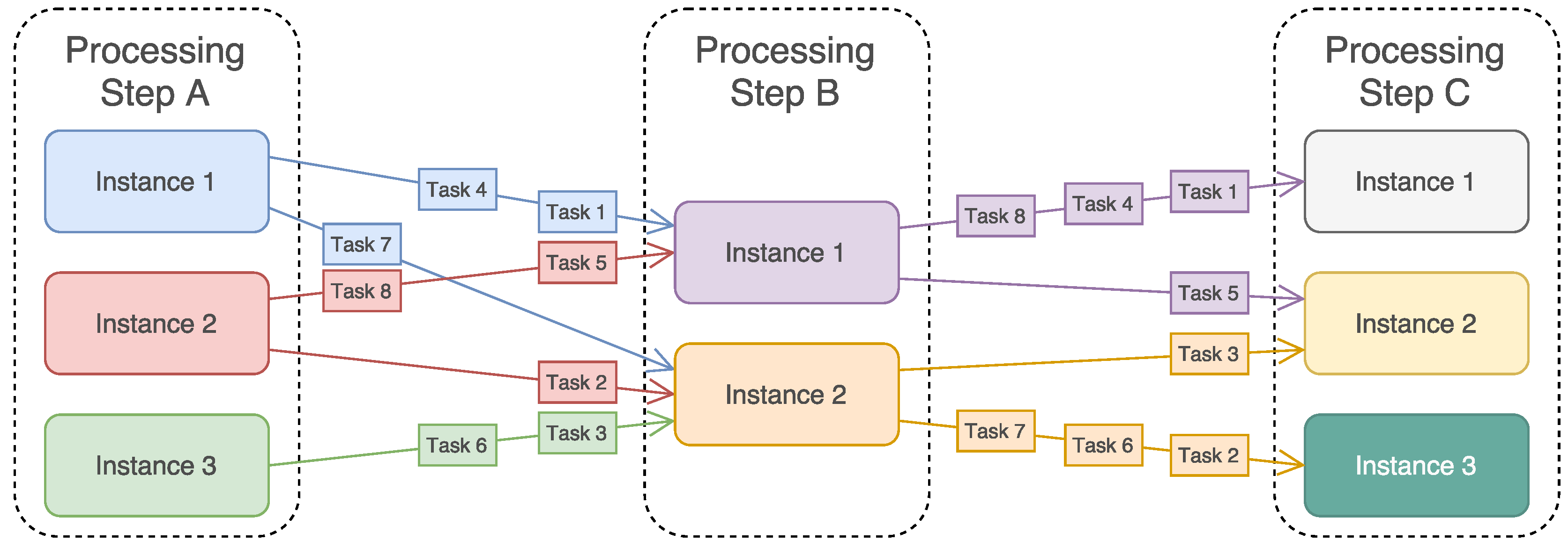
For clarification purposes, first, the relevant terms for this work are explained. The type of applications that this work is aimed at are processing chains, which are formed by chaining processing steps so that the output of a step is linked to the input of the next step in the chain, except for the first and last steps. Processing steps are, in turn, formed by a number of processing step instances. Tasks are single entities that contain the data that are processed at the processing step instances. In Figure 1, an overview is shown with an example of a processing chain that will be used throughout this paper.
The rest of this section explains our approach to reducing the under-utilization of resources in a heterogeneous computational cluster. First, a general idea is described on how to classify successive steps in a processing cChain. Subsequently, the optimal distribution of processing steps is calculated which, in turn, is used to calculate the number of worker instances necessary. Last, the calculation of the number of resources needed for each resource type is performed. To provide more clarification, a worked out example of the solution is provided in Section 3.4.
In order to estimate the optimal distribution of resources, we need to make sure that none of the steps in the Processing Chain are under- or over-producing. As this is the cause for resource under-utilization when processing steps require different resources. Looking at the structure of the applications used in this paper, it can be observed that computations are composed of a series of steps that are chained together by attaching the output of one step to the input of another step. Steps, therefore, produce the input for a step that is consuming that input. Because the steps are chained, one step is both a consumer and a producer, except for the first and the last steps in the chain. To investigate the efficiency of processing chains, we identified the metrics based on the notion that the input is split up into relatively small tasks, shown in Table 1, that can help us to determine the utilization of individual steps in the chain. The metrics were gathered for a given interval, the PublishWait and ConsumeWait metrics were averaged over this interval for all tasks processed in that interval.
There are three categories to which a pair of Processing Steps can be classified with respect to the rate of production and consumption of data:
- Fast producer, slow consumer: The producer is producing at a higher rate than the consumer is able to consume.
- Slow producer, fast consumer: The consumer is consuming at a higher rate than the producer is able to produce.
- Balanced producer and consumer: The rates of producing and consuming are balanced.
Table 1 provides an overview of the classification of a pair of processing steps. Combining the metrics from Table 1 and these categories, a pair of processing steps can be classified with respect to the flow of input/output data between them. An overview of the metrics and categories is shown in Table 2. The pathological state is a special category to which two steps in normal operations cannot reach. For example, there is no logical explanation for two steps waiting on each other, as the publishers local buffer is full and the consumer is waiting for tasks to appear in that same local buffer.
3.1. Processing Chain Distribution
When the processing steps are categorized into the different states, determination of the ratio between the steps should occur. For this, the currently deployed ratio between the processing steps is needed; this is provided by Equation (1), where n is the number of instances for either the producing processing step or the consuming processing step:
Calculation of the new ratio depends on the category that the pair of processing steps falls into (see Table 2) as well as the BufferChange. The category determines whether there should be more or less publishers relative to consumers, and the buffer change indicates whether or not the buffer is full or empty. If the buffer is not full and not empty, the change in the buffer can be used to determine the optimal ratio between the processing steps. The BufferChange is 2 when the producers process 2 times more tasks than the consumers is consuming, and it is when the consumers consume tasks 2 times faster than the producer is producing. Multiplying the number of consumers by the BufferChange results in an increase in workers when the producer is faster and a decrease of workers when the consumer is faster, which is the goal of calculating the ratios between processing steps.
When the buffer is full, either the producer has a significant wait percentage to publish tasks in its buffer, or the consumer is exactly on par with the production of the producer. In cases where the producer is waiting, it makes sense to lower the amount of producer instances with the percentage that the producers are waiting on average. The same holds for cases where the buffer is empty and consumers are waiting for significant amounts of time for new tasks; in these cases, the number of consumer instances should be lowered.
In Equations (2)–(6), this description is translated into formulas that can be used in algorithms later on:
where = BufferChange, pw = PublishWait, cw = ConsumeWait.
With the new set of ratios for the processing chain, the distribution can be calculated with an recursive function, as displayed in Equation (7):
where D is the distribution of processing steps.
For each processing step in the processing chain, the position in the chain determines which D belongs to that Processing Step, e.g., for the configuration shown in Figure 1, this is 3:2:3. The first processing step has an index of 1, and the last processing step has an index of N. For clarification, D is normalized against the sum of D, following Equation (9):
The normalized distribution, , now contains the fraction of instances that a processing step needs with respect to the total number of instances.
3.2. Processing Step Instance Counts
The normalized distribution, , can be used to determine the amount of instances that each processing step is to be assigned that will improve the resource utilization. For this, the resource utilization metric Utilization is needed. This metric defines the utilization of a resource, and, therefore, the ability of that resource to handle more tasks. To be able to use the utilization in formulas, a function was introduced in Equation (10) that returns the fraction of utilization of an input processing step, which corresponds with the utilization of the resource that is needed for that processing step. The utilization measured is the utilization at the moment of calculation, with possibly a small interval to overcome sudden peaks or drops in the utilization depending on how the metrics are gathered:
This function is used to determine the scaling factor that results in the total amount of instances that at least can run on the specific resource, by dividing the current amount of instances by the utilization fraction. As the current amount of instances do not produce more load than the current utilization fraction, scaling the amount of instances by 1 over the utilization of the instances that cannot produce more than the current load as is always equal to 1. Equation (11) shows the calculation of the scale factor which is determined for all processing steps that have an higher distribution factor than that currently deployed:
As all of the processing steps are scaled based upon the same scale factor, the lowest scale factor should be used, as this is the scale factor that leads to no over-utilization of the processing steps, because, when a scaling factor is chosen not to be the minimum, scaling the resource with the highest utilization with this factor will lead to an utilization higher than 1. With these factors calculated, the new processing step instance count can be determined. By following Equation (12), the new set of processing step instance counts can be calculated:
where = # current instances of step p.
This set, , can now be used to scale the processing step instance. As contains fractions, the set must most likely be converted to a set of number of workers by either rounding, ceiling, or flooring the fractions, depending on the characteristics of the processing step instances and the kind of resources used in the processing chain.
3.3. Resource Provisioning
At this stage, the processing step instance count is stable, meaning that the resource usage is fairly constant, so the optimal resource distribution can be determined. By multiplying the number of resource instances by the utilization factor, the optimal number of instances for the current situation can be calculated. As the number of processing step instances, , will not use more than 100% of the resources, none of the resources are over-utilized at this moment. As for the calculation of the normalized distribution of processing step instances, , for the resource distribution, a normalized distribution is used to make the calculations using the distribution easier, as shown in Equation (13):
where is the # current instances of resource r, and is the utilization of resource r.
To determine the extent to which the resource instances should be scaled up or down, a budget per time unit, B, of the maximal resource allocation is needed. Calculating the number of resource instances that is needed to create an even resource utilization is a simple task, as shown in Equation (14):
This new optimal resource instance count, , is fractional, as resources are most likely scaled based on integers, so the fractions have to be converted to corresponding integers.
3.4. Example
To clarify the formulas, a synthetic scenario was worked out based on a car manufacturing process. This scenario has a logical heterogeneity in the resources and provides a clear abstraction of our problem space. In the scenario, four processing steps were distinguished: the dealer, body processing, painting, and assembly. In Table 3, the metrics of the processing steps at a given point are shown, when, in the current configuration, there is an imbalance of resources.
Each of the processing steps uses a distinct resource, so four utilization metrics are shown in Equation (15) with their corresponding scale factors.
The initial ratios were determined from the number of instances from Table 3, as shown in Equation (16):
Now, given the initial ratios and the metrics at a certain point in time, the new processing step distribution was calculated. All the ratios are in the form of to improve readability in the following equations. Equation (17) shows these calculations and their results:
Given these ratios, the distribution of processing steps was determined, as shown in Equation (18), where the values of correspond to the consumers of each pair of processing steps. So, the value of corresponds to the body processing instances, and corresponds to the painting instances. The last value, , corresponds to the consumers of the first processing step, namely, the dealer:
Normalizing this distribution gave the fractions of each processing step, as shown in Equation (19), which sums up to 1. This indicates that, in this case, all of the processing step instances should be of the body processing type:
Once the new processing step distribution had been calculated, the processing step instance count could be determined. First the starting point for the scaling was determined by looking at the resource that is utilized the most, which is the resource belonging to the body processing step, as shown in Equation (20):
Filling in Equation (12) with the calculated values gave the new processing step instance distribution. Using Equation (21), the values of the desired instance counts were calculated:
As these numbers are fractional and it is most likely that we could not use half a paint gun, these values were rounded up to the next integer. Table 4 shows the number of processing step instances that should be provisioned.
4. Reference Platform Architecture
Using the solution for calculating the distributions of processing step instances as well as resources, we now discuss a reference platform architecture that incorporates the concepts of the previous section combined with a control loop that continuously applies these concepts. We use micro-batching in order to retrieve application metrics in a timely manner. This enables us to demonstrate a proof of concept that is able to evaluate these concepts.
The high-level architecture of the platform, shown in Figure 2, gives an overview of the components in the platform and the relationships between these components. The logical center of the platform is the monitor, which monitors running processing chains and make decisions for the provision of processing step instances as well as resource instances. The monitor has no direct notion of the resources and processing step instances; separate managers (i.e., resource or processing step managers in Figure 2) provide a layer of abstraction for these components. This allows letting these managers take care of the low-level matching between processing step instances and resources and letting the monitor take decisions on the global overview of the processing chains. It also offers the option to change resource managers or processing step managers to other vendors.
The monitor orchestrates processing chains, by initializing, monitoring, and modifying processing chains initiated by users, based on the algorithms proposed in Section 3. Dynamic provisioning is provided by the monitor, as this component gathers the metrics of the resources and the processing step instances. The monitor is, therefore, responsible for the control loop for the processing chain, specifically, monitoring and controlling the processing chain. The architecture of the run-time monitoring and coordination, as shown in Figure 3, provides a solution for the distribution and scheduling of tasks. Furthermore, the run-time architecture provides information on how the processing chain metrics are gathered.
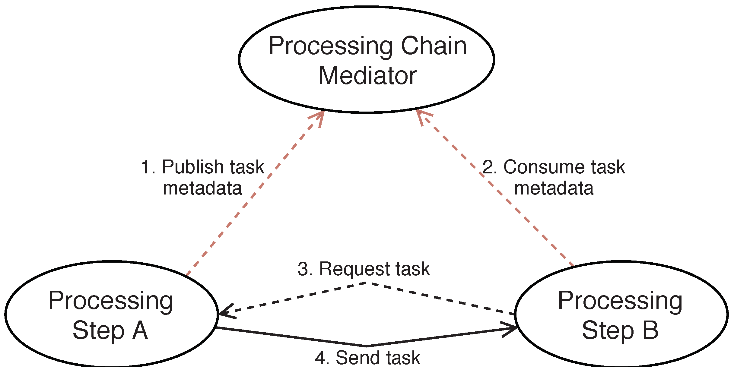
Processing chains delegate the execution of computations to processing step instances to execute functions on input data. In order to manage the distribution of tasks across processing step instances, processing chain mediators are introduced. These mediators are responsible for distributing the tasks that they receive to processing step instances for the next processing step. To prevent the mediators becoming a bottleneck when all data travels through them, only task descriptions are shared with the mediators. These task descriptions are small packages, indicating that the processing step that published the task description has a new task available. Processing step instances have the responsibility of transferring the data between each other. The reason that mediators are situated between the processing step instances is because the monitor is required to know how tasks are traveling through the system so that it has an accurate view of the running processing chain. The mediators share the knowledge they have about the processing chain section they are responsible for. In Figure 3, the communication steps between the processing step instances and mediators is shown. The dotted lines indicate that the amount of network traffic used is small compared to the solid line. The communication over the dotted lines are meta-data of the tasks. The time it takes to transfer and process these messages is a couple of magnitudes lower than the time it takes to transfer and process the actual tasks.
The control loop that periodically decides on the distribution of processing step instances and resource instances is mainly situated at the monitor, which controls the number of instances for both the processing steps and the resources. To be able to calculate new instance counts requires the algorithm discussed in Section 3, which provides run-time feedback based on the number of instances deployed at that moment.
The processing chain metrics are gathered for all partitions during the application run-time. Therefore, we use micro-batching to ensure that the processing time of single partitions is relatively low. The interval of the control loops depends mainly on external factors from resource providers, as the time to provision resources depends heavily on the types of resources. Furthermore, the gathering of metrics from the resources introduces additional delays, as the metrics provided by the resource providers are not instantaneous.
5. Experiments
To evaluate the effectiveness of the solution and the architecture, a scenario from the Netherlands Organisation for Applied Scientific Research (TNO) project sensor-technology applied to underground pipeline-infrastructures (STOOP) [27], with an existing approach using Apache Spark is used. In this project, sensor-technology was used to estimate the chance on underground pipeline failures based on the land subsidence around pipelines in the future. An example of the scenario used in the STOOP project is shown in Algorithm 1. In this scenario, the underground pipeline is divided into segments that are calculated individually. For each segment, a Monte Carlo algorithm is used to variate the model inputs. For each variation, the region layout is generated which is used as input for the land subsidence model and the pipeline soil spring model. The results of these models are combined and serve as inputs for the underground pipeline stress model; based on these stresses, a Boolean output is given that indicates whether or not the pipeline is likely to fail.
| Algorithm 1 STOOP model pseudo-code |
|
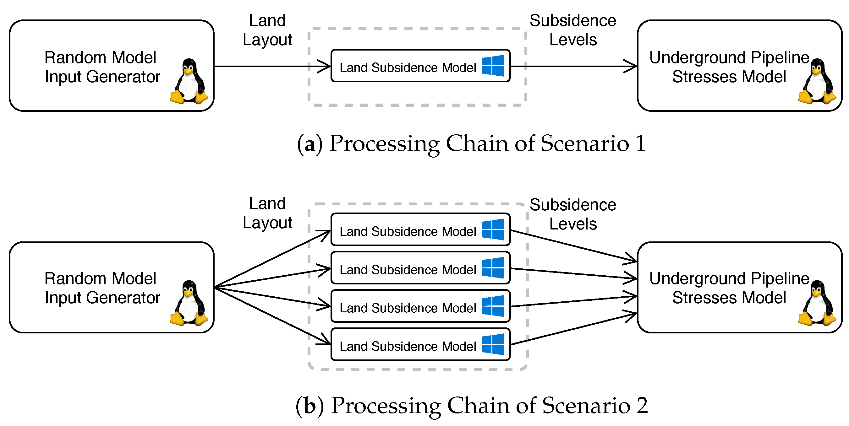
A simplification of this model is used to evaluate our solution. In Figure 4, this processing chain is shown. The model calculates the land subsidence of soil in the area of a pipeline after a given period of time given a weight, i.e., extra soil, that is added; based on this land subsidence, the stresses on the pipeline are estimated. There are two types of resources used in this processing chain: a Linux resource type for the model input generator and the underground pipeline stresses model and a Windows resource type for the land subsidence model.
The input generator and the underground pipeline stresses model are both Linux models, and the land subsidence model is a Windows model. Three different scenarios based on the test case were evaluated as follows:
- Scenario 1: A single model input was introduced to the land subsidence model, so only one land subsidence calculation was needed per pipeline segment.
- Scenario 2: Four model inputs were introduced to the land subsidence model, so four land subsidence calculations were needed per pipeline segment.
- Scenario 3: Starting similar as Scenario 1, but halfway switching to Scenario 2.
The calculation times of each land subsidence calculation were roughly half the time of a pipeline stress calculation, respectively the second and third step in Figure 4. The random model input generator is negligible with respect to the other two models.
All of the test scenarios were performed on an Azure cluster with 20 virtual machines (VMs) allocated to each test run, for 5 runs per scenario. For the first scenario, additional tests were performed with 100 VMs for 3 runs to verify the scalability of the platform itself. The number of tasks processed in this scenario was 10 times higher than for the 20 VM tests. The VMs were Standard D2 v3 (https://azure.microsoft.com/en-us/pricing/details/cloud-services/) Azure instances with two cores and 8GB of RAM. All tests were run in the same Azure Europe West region, to maintain the best network connectivity between VMs. One additional VM was used in each scenario to run the monitor and user interface for the platform. The tests started with a fraction of the VM budget, preventing the removal of resources at the beginning of the executions. For the test with a budget of 20 VMs, the test started with 4 VMs, evenly distributed over Windows and Linux. For the tests with a 100 VM budget, the tests started with 10 VMs.
For comparison, an alternative solution using Apache Spark (version 2.2.0) was used as the baseline. This alternative deploys a Linux Spark cluster which propagates calculations for the land subsidence model to a partner VM running Windows which results in a fixed cluster with, in the case of the 20 VMs test runs, 10 Linux VMs and 10 Windows VMs. This approach is currently used in the project, and, therefore, is a good approach to compare the adaptive approach with.
5.1. Results
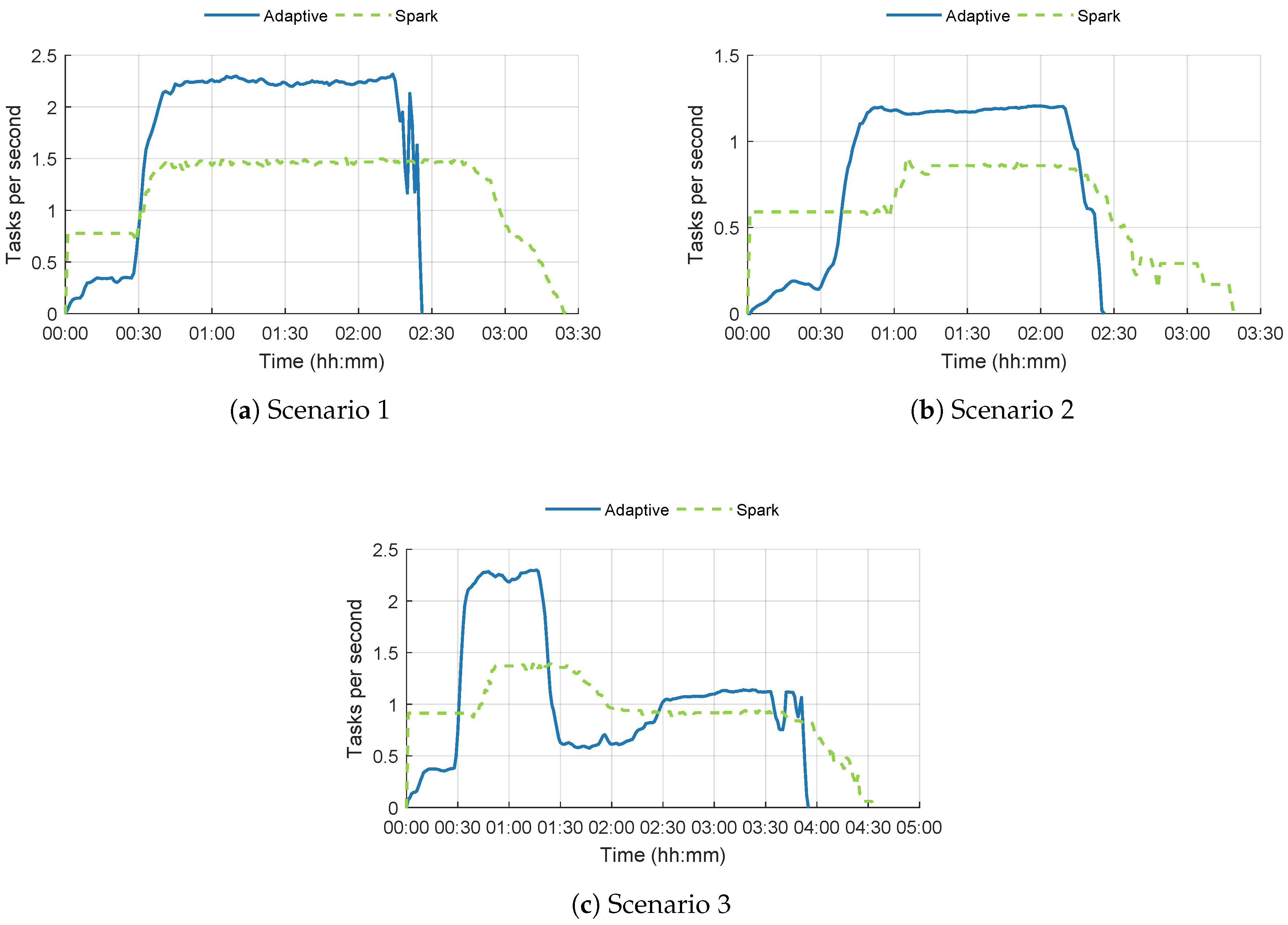
In Figure 5, the results of the tests with 20 VMs for all scenarios are shown with respect to the throughput of tasks in the platform. In Figure 5a–c, similar patterns arise—at first our adaptive platform performs worse than the reference Spark solution. This is easily explained by the fact that less VMs have started at the beginning of the test runs on the adaptive platform. After roughly 30 min, the additional VMs start which leads to a significant increase in the throughput of the adaptive platform. The Spark solution also shows a lower throughput at the beginning of the test runs; this is because provisioning the land subsidence model takes around 20 to 30 min. This is due to the fact that provisioning a Windows VM takes longer than Linux VMs as well as the fact that downloading and starting the land subsidence model takes longer than the Linux counterparts. In the following tasks that are executed, this model is already loaded so that throughput of tasks is higher. For the third scenario, it is clear that the throughput of the adaptive platform drops below the Spark throughput; this is explained by the fact that the distribution is skewed towards the first phase of the test scenario and therefore, performs worse when the second phase of tasks is launched.
The overall results of the tests with 20 VMs are shown in Table 5. The improvement in the throughput is measured at the time periods when both approaches were relatively stable with respect to the throughput of tasks. For the three scenarios, these were, respectively, 0:45–2:15, 1:15–2:15, and 0:45–1:15 & 2:30–3:30. It is clear that, in the third scenario, the improvement in the adaptive approach was the lowest; this is due to the costs of reconfiguring the resources two times. The longer the scenario is, the more benefits the adaptive approach can provide.
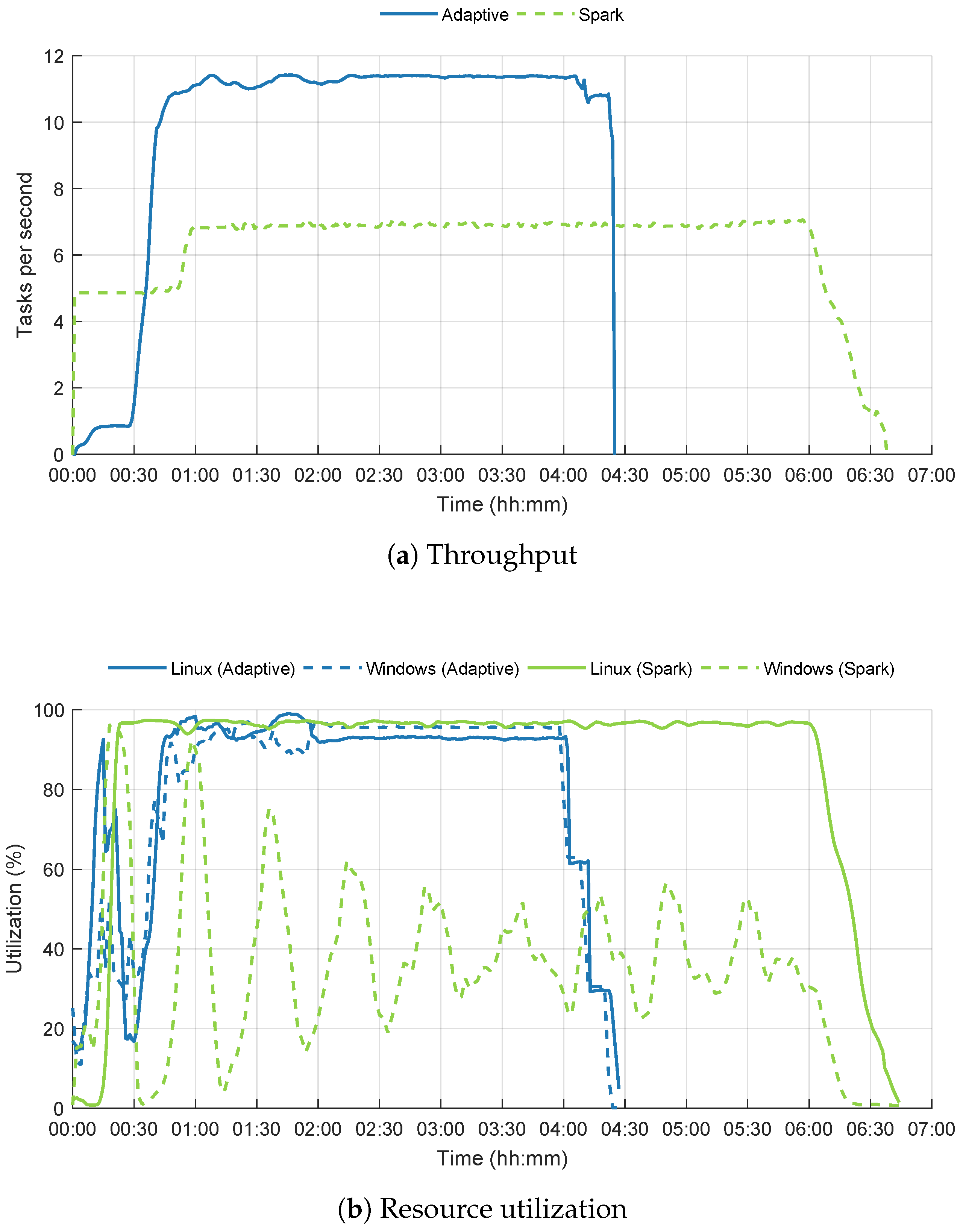
To verify the scalability of the adaptive approach, the first scenario was also run with 100 VMs. In Figure 6, the throughput and resource utilization are shown. The throughput figure is similar to Figure 5a, but the advantage of the adaptive approach is shown to be even higher with 100 VMs compared to 20 VMs.
Looking at the resource utilization of the cluster, the adaptive approach exceeds an average utilization of 90% after 45 min. Instead, the Spark approach reaches, on average, around 65% resource utilization. This explains the reduced lead time of more than 2 h from the 6.5 h required during baseline.
During testing, in both approaches we saw that deploying larger amounts of VMs on Azure led to approximately 3% to 5% of VMs not provisioning correctly. This could be overcome for the adaptive approach by enabling the over-provisioning feature of Azure, so that more VMs are started. This feature monitors the amount of VMs that are provisioned successfully, and when the desired amount of VMs are provisioned successfully it removes the VMs that are still busy with provisioning. For the Spark approach, this was not possible, because in this approach, two VMs are linked to each other and when one of the VMs in such a link is not provisioned correctly, both VMs will not process tasks. So, more VMs are provisioned and the excess VMs have to be removed manually from the cluster to achieve a more optimal number of working VMs.
It is also interesting to compare the costs of the tests with 100 VMs as they are run on Microsoft Azure. To estimate the cost improvement of the tests, the number of VM hours has to be determined. For the Spark scenario, this is easy, as its tests ran for 404 min with 50 Linux VMs and 50 Windows VMs. For the adaptive approach, a calculation had to be made for each window between the provision steps. The results of this calculation are shown in Table 6. In this table, the execution costs are also displayed, based on the pricing on 27 September, 2017, i.e., $0.212 per hour per VM for Windows VMs and $0.120 per hour per VM for Linux VMs for the selected configuration of Azure Standard D2 VM.
The large difference in costs, with an improvement of almost 45%, can partly be explained by the fact that, in the Spark approach, the Windows VMs were not utilized optimally since Windows VMs are almost twice as costly as Linux VMs.
5.2. Discussion
The results of the experiments are very promising with significant improvements with respect to throughput, resource utilization, and lead time. In particular, when scenarios take at least several hours and the platform is relatively stable, the resource utilization approaches 95%. As seen in the third scenario, the platform is able to adapt to changing demands for resources, although, in this scenario, following the sudden switch from a higher demand for Linux to a higher demand for Windows, it took almost an hour to re-balance the cluster correctly.
However, there are some difficulties with this approach with respect to the provisioning of new resources. For example, the time between deciding a new Windows VM needed to be started and the moment it is ready and available to the processing chain can be up to 30 min. Furthermore, the failure rate for provisioning resources is for such clusters is on a level at which special actions have to be taken in order to ensure the overall state of the cluster. When looking at the resource utilization in the case of 100 VMs (Figure 6b), it takes 2 h for the platform to stabilize. Although it reaches it reaches the maximum throughput after 45 min. This is, however, a limitation of the computational infrastructure, but the approach still works and should work even better when computational infrastructures have evolved.
Another limitation at this point is the gathering of metrics of resources. For the Azure cloud metrics, the smallest interval is 1 minute, and the delay of the metrics is 2–3 min. So, the decision-making process occurs quite some time after the actual state of the cluster.
6. Conclusions
This work introduced a new approach to the adaptive provision of heterogeneous resources based on demand at run-time. By estimating the distributions between steps in a processing chain, the workers can be balanced, and resources can be provisioned accordingly. By using these distributions in a control loop that continuously monitors applications at run-time, an adaptive computing environment is created that is altered to match application demand. A reference platform was created to allow the evaluation of our approach with respect to an industrial use case.
Our approach showed very promising results. By increasing the overall utilization of resources, significant improvements in lead time and task throughput were realized, as shown in Figure 5 and Figure 6.
The basis behind the approach is quite intuitive—by introducing small buffers between processing steps, the relative performance of two linked processing steps can be estimated by using this information, to deploy the right amount of resources as well as processing step instances; thus, a balanced ecosystem is created.
However, reconfiguring cloud resources can still take up to 20 min before resources are fully operational, or even longer when a large number of resources is requested. In particular, in the case of Windows VMs, the land subsidence model took quite some time to successfully provision. This means that the approach is less useful for applications with small lead times, or in which the distribution of resources changes often. In the experiments conducted, we found that the lead time should be at least around 10 times the time it takes to reconfigure resources, especially when the distribution of resources is likely to change heavily during one run, like we saw in the third scenario where the reconfiguration took quite some time. However, for the third scenario, there was also an improvement in lead time of 14%.
This paper provides a new approach to data processing with heterogeneous resources. Different aspects could be identified in further research to improve the results of this approach. Data locality is one of those aspects—for this research we focused on CPU intensive tasks as the amount of data that has to be transferred is low compared to the computational time. For this approach to be suitable for data intensive tasks, data locality should be taken into account. By performing computations as close to the data as possible, the performance loss in transferring data can be reduced. However, when heterogeneous resources are used, the data has to be moved to the corresponding platform which is unavoidable. Corresponding to the aspect of data locality, support for distributed file systems and databases should be added to fully support big data processing by optimizing the decision-making process and having a higher frequency of metric gathering. The latter can only be achieved when cloud platforms provide these data at higher rates, but incorporating another system for metrics gathering could also improve the frequency of metrics.
Author Contributions
M.K., A.L., V.A., E.H. and E.L. conceived the idea. A.L. and V.A. were involved in planning and supervised the work. M.K, E.H. and E.L. designed and performed the experiments. M.K. wrote the manuscript with input from all authors.
Funding
This research received no external funding.
Conflicts of Interest
The authors declare no conflict of interest.
References
- Carolina Donnelly. Public Cloud Competition Prompts 66 Research Reveals. 2016. Available online: https://www.computerweekly.com/news/4500270463/Public-cloud-competition-results-in-66-drop-in-prices-since-2013-research-reveals (accessed on 31 May 2018).
- Toyota. Toyota Production System. Available online: https://www.toyota-europe.com/world-of-toyota/this-is-toyota/toyota-production-system (accessed on 31 May 2018).[Green Version]
- Microsoft Azure. Overview of Autoscale with Azure Virtual Machine Scale Sets. 2018. Available online: https://docs.microsoft.com/en-us/azure/virtual-machine-scale-sets/virtual-machine-scale-sets-autoscale-overview (accessed on 31 May 2018).
- Amazon Web Services. Overview of Autoscale with Azure Virtual Machine Scale Sets. Available online: https://docs.aws.amazon.com/autoscaling/ec2/userguide/what-is-amazon-ec2-auto-scaling.html (accessed on 31 May 2018).
- Dean, J.; Ghemawat, S. MapReduce: Simplified Data Processing on Large Clusters. In Proceedings of the 6th Conference on Symposium on Opearting Systems Design & Implementation (OSDI’04), San Francisco, CA, USA, 6–8 December 2004; USENIX Association: Berkeley, CA, USA, 2004; Volume 6, p. 10. [Google Scholar]
- Ahmad, F.; Chakradhar, S.T.; Raghunathan, A.; Vijaykumar, T.N. Tarazu. In Proceedings of the Seventeenth International Conference on Architectural Support for Programming Languages and Operating Systems (ASPLOS ’12), London, UK, 3–7 March 2012; ACM Press: New York, NY, USA, 2012. [Google Scholar] [CrossRef]
- Cheng, D.; Zhou, X.; Lama, P.; Wu, J.; Jiang, C. Cross-Platform Resource Scheduling for Spark and MapReduce on YARN. IEEE Trans. Comput. 2017, 66, 1341–1353. [Google Scholar] [CrossRef]
- Burton, F.W.; Sleep, M.R. Executing functional programs on a virtual tree of processors. In Proceedings of the 1981 Conference on Functional Programming Languages and Computer Architecture (FPCA ’81), Portsmouth, NH, USA, 18–22 October 1981; ACM Press: New York, NY, USA, 1981. [Google Scholar] [CrossRef]
- Acar, U.A.; Chargueraud, A.; Rainey, M. Scheduling parallel programs by work stealing with private deques. In Proceedings of the 18th ACM SIGPLAN Symposium on Principles and Practice of Parallel Programming (PPoPP ’13), Shenzhen, China, 23–27 February 2013; ACM Press: New York, NY, USA, 2013. [Google Scholar] [CrossRef]
- Zaharia, M.; Konwinski, A.; Joseph, A.D.; Katz, R.; Stoica, I. Improving MapReduce Performance in Heterogeneous Environments. In Proceedings of the 8th USENIX Conference on Operating Systems Design and Implementation (OSDI’08), San Diego, CA, USA, 8–10 December 2008; USENIX Association: Berkeley, CA, USA, 2008; pp. 29–42. [Google Scholar]
- Xing, Y.; Zdonik, S.; Hwang, J.H. Dynamic load distribution in the Borealis stream processor. In Proceedings of the 21st International Conference on Data Engineering (ICDE’05), Tokoyo, Japan, 5–8 April 2005; pp. 791–802. [Google Scholar] [CrossRef]
- Shah, M.A.; Hellerstein, J.M.; Chandrasekaran, S.; Franklin, M.J. Flux: An adaptive partitioning operator for continuous query systems. In Proceedings of the 19th International Conference on Data Engineering (Cat. No.03CH37405), Bangalore, India, 5–8 March 2003; pp. 25–36. [Google Scholar] [CrossRef]
- Collins, R.L.; Carloni, L.P. Flexible filters. In Proceedings of the Seventh ACM International Conference on Embedded Software (EMSOFT ’09), Grenoble, France, 11–16 October 2009; ACM Press: New York, NY, USA, 2009. [Google Scholar] [CrossRef]
- Cheng, D.; Chen, Y.; Zhou, X.; Gmach, D.; Milojicic, D. Adaptive scheduling of parallel jobs in spark streaming. In Proceedings of the Conference on Computer Communications (INFOCOM 2017), Atlanta, GA, USA, 1–4 May 2017; IEEE: Piscataway Township, NJ, USA, 2017. [Google Scholar] [CrossRef]
- Pace, F.; Venzano, D.; Carra, D.; Michiardi, P. Flexible Scheduling of Distributed Analytic Applications. In Proceedings of the 2017 17th IEEE/ACM International Symposium on Cluster, Cloud and Grid Computing (CCGRID), Madrid, Spain, 14–17 May 2017; IEEE: Piscataway Township, NJ, USA, 2017. [Google Scholar] [CrossRef]
- Ostermann, S.; Prodan, R.; Fahringer, T. Dynamic Cloud provisioning for scientific Grid workflows. In Proceedings of the 2010 11th IEEE/ACM International Conference on Grid Computing, Brussels, Belgium, 25–28 October 2010; IEEE: Piscataway Township, NJ, USA, 2010. [Google Scholar] [CrossRef]
- Buyya, R.; Barreto, D. Multi-cloud resource provisioning with Aneka: A unified and integrated utilisation of microsoft azure and amazon EC2 instances. In Proceedings of the 2015 International Conference on Computing and Network Communications (CoCoNet), Kerala, India, 16–19 December 2015; IEEE: Piscataway Township, NJ, USA, 2015. [Google Scholar] [CrossRef]
- Zhang, Q.; Cherkasova, L.; Smirni, E. A Regression-Based Analytic Model for Dynamic Resource Provisioning of Multi-Tier Applications. In Proceedings of the Fourth International Conference on Autonomic Computing (ICAC’07), Jacksonville, FL, USA, 11–15 June 2007; IEEE: Piscataway Township, NJ, USA, 2007. [Google Scholar] [CrossRef]
- Zhang, Q.; Zhani, M.F.; Boutaba, R.; Hellerstein, J.L. Dynamic Heterogeneity-Aware Resource Provisioning in the Cloud. IEEE Trans. Cloud Comput. 2014, 2, 14–28. [Google Scholar] [CrossRef]
- Xu, D.; Liu, X.; Fan, B. Efficient Server Provisioning and Offloading Policies for Internet Data Centers with Dynamic Load-Demand. IEEE Trans. Comput. 2015, 64, 682–697. [Google Scholar] [CrossRef]
- Maroulis, S.; Zacheilas, N.; Kalogeraki, V. A Framework for Efficient Energy Scheduling of Spark Workloads. In Proceedings of the 2017 IEEE 37th International Conference on Distributed Computing Systems (ICDCS), Atlanta, GA, USA, 5–8 June 2017; IEEE: Piscataway Township, NJ, USA, 2017. [Google Scholar] [CrossRef]
- Peinl, R.; Holzschuher, F.; Pfitzer, F. Docker Cluster Management for the Cloud—Survey Results and Own Solution. J. Grid Comput. 2016, 14, 265–282. [Google Scholar] [CrossRef]
- Verma, A.; Pedrosa, L.; Korupolu, M.; Oppenheimer, D.; Tune, E.; Wilkes, J. Large-scale cluster management at Google with Borg. In Proceedings of the Tenth European Conference on Computer Systems (EuroSys ’15), Bordeaux, France, 21–24 April 2015; ACM Press: New York, NY, USA, 2015. [Google Scholar] [CrossRef]
- Zheng, C.; Thain, D. Integrating Containers into Workflows. In Proceedings of the 8th International Workshop on Virtualization Technologies in Distributed Computing (VTDC ’15), Portland, OR, USA, 15–16 June 2015; ACM Press: New York, NY, USA, 2015. [Google Scholar] [CrossRef]
- Liu, K.; Aida, K.; Yokoyama, S.; Masatani, Y. Flexible Container-Based Computing Platform on Cloud for Scientific Workflows. In Proceedings of the 2016 International Conference on Cloud Computing Research and Innovations (ICCCRI), Singapore, 4–5 May 2016; IEEE: Piscataway Township, NJ, USA, 2016. [Google Scholar] [CrossRef]
- Zhao, Y.; Li, Y.; Raicu, I.; Lu, S.; Tian, W.; Liu, H. Enabling scalable scientific workflow management in the Cloud. Future Gener. Comput. Syst. 2015, 46, 3–16. [Google Scholar] [CrossRef]
- TNO. Innovative Techniques for Monitoring Infrastructures. Available online: https://www.tno.nl/en/focus-areas/information-communication-technology/roadmaps/information-creation-from-data-to-information/innovative-techniques-for-monitoring-infrastructures/ (accessed on 31 May 2018).
Figure 1.
Flow of tasks through a processing chain.

Figure 2.
High-level architecture.

Figure 3.
Run-time task distribution.

Figure 4.
Processing chains of the test scenarios; Scenario 3 is a composition and acts as Scenario 1 for the first half of the tasks and as Scenario 2 for the remainder of the tasks.
Figure 4.
Processing chains of the test scenarios; Scenario 3 is a composition and acts as Scenario 1 for the first half of the tasks and as Scenario 2 for the remainder of the tasks.

Figure 5.
Throughput of the three scenarios with 20 VMs over 5 runs.

Figure 6.
Scenario 1 with 100 VMs over 3 runs.


Table 1.
Processing chain metrics.
| Metric Code | Formula | Description |
|---|---|---|
| PublishWait | The ratio of wait time to publish a task in the local buffer () of producing processing steps, to the processing time of that task (). | |
| BufferChange | The ratio of the number of tasks being published to the local buffer to the number of tasks transferred to consumers. | |
| ConsumeWait | The ratio of the wait time for a new task () to the processing time of that task () for consuming processing steps. |
Table 2.
Producer/consumer categorization, indicating in which category the producer and consumer belong to with the following possibilities: fast producer slow consumer (FP-SC), slow producer fast consumer (SP-FC), balanced producer and consumer (Balanced), and pathological states (-).
Table 2.
Producer/consumer categorization, indicating in which category the producer and consumer belong to with the following possibilities: fast producer slow consumer (FP-SC), slow producer fast consumer (SP-FC), balanced producer and consumer (Balanced), and pathological states (-).
| BufferChange | ||||
|---|---|---|---|---|
| PublishWait | ConsumeWait | <1 | ≈1 | >1 |
| ≈0 | ≈0 | SP-FC | Balanced | FP-SC |
| ≈0 | >0 | - | SP-FS | - |
| >0 | ≈0 | - | FP-SC | - |
| >0 | >0 | - | - | - |
Table 3.
Scenario metrics.
| Processing Step | Instances | PublishWait | BufferChange | ConsumeWait |
|---|---|---|---|---|
| Dealer | 1 | ≈1 | ||
| Body processing | 20 | ≈1 | ≈0 | |
| Painting | 5 | ≈0 | 1.2 | ≈0 |
| Assembly | 10 | ≈0 | ≈1 | ≈0 |
Table 4.
New instance counts.
| Processing Step | # Instances |
|---|---|
| Dealer | 1 |
| Body processing | 50 |
| Painting | 14 |
| Assembly | 6 |
Table 5.
Improvements of the adaptive approach relative to the Spark approach.
| Scenario | Throughput | Resource Utilization | Lead Time |
|---|---|---|---|
| 1 | 50% | 30% | 29% |
| 2 | 40% | 29% | 27% |
| 3 | 57% & 22% | 8.3% | 14% |
Table 6.
Costs of different approaches on Microsoft Azure.
| Approach | VM Hours (Windows, Linux) | Costs (Windows + Linux) |
|---|---|---|
| Adaptive | , | |
| Spark | , |
© 2018 by the authors. Licensee MDPI, Basel, Switzerland. This article is an open access article distributed under the terms and conditions of the Creative Commons Attribution (CC BY) license (http://creativecommons.org/licenses/by/4.0/).
Share and Cite
MDPI and ACS Style
Kollenstart, M.; Harmsma, E.; Langius, E.; Andrikopoulos, V.; Lazovik, A. Adaptive Provisioning of Heterogeneous Cloud Resources for Big Data Processing. Big Data Cogn. Comput. 2018, 2, 15. https://doi.org/10.3390/bdcc2030015
AMA Style
Kollenstart M, Harmsma E, Langius E, Andrikopoulos V, Lazovik A. Adaptive Provisioning of Heterogeneous Cloud Resources for Big Data Processing. Big Data and Cognitive Computing. 2018; 2(3):15. https://doi.org/10.3390/bdcc2030015
Chicago/Turabian StyleKollenstart, Maarten, Edwin Harmsma, Erik Langius, Vasilios Andrikopoulos, and Alexander Lazovik. 2018. "Adaptive Provisioning of Heterogeneous Cloud Resources for Big Data Processing" Big Data and Cognitive Computing 2, no. 3: 15. https://doi.org/10.3390/bdcc2030015