Breast Cancer Diagnosis System Based on Semantic Analysis and Choquet Integral Feature Selection for High Risk Subjects

Abstract

In this work, we build a computer aided diagnosis (CAD) system of breast cancer for high risk patients considering the breast imaging reporting and data system (BIRADS), mapping main expert concepts and rules. Therefore, a bag of words is built based on the ontology of breast cancer analysis. For a more reliable characterization of the lesion, a feature selection based on Choquet integral is applied aiming at discarding the irrelevant descriptors. Then, a set of well-known machine learning tools are used for semantic annotation to fill the gap between low level knowledge and expert concepts involved in the BIRADS classification. Indeed, expert rules are implicitly modeled using a set of classifiers for severity diagnosis. As a result, the feature selection gives a a better assessment of the lesion and the semantic analysis context offers an attractive frame to include external factors and meta-knowledge, as well as exploiting more than one modality. Accordingly, our CAD system is intended for diagnosis of breast cancer for high risk patients. It has been then validated based on two complementary modalities, MRI and dual energy contrast enhancement mammography (DECEDM), the proposed system leads a correct classification rate of 99%.

1. Introduction

Breast cancer is a malignant lesion of the mammary gland. Several risk factors exist, and could raise the risk of its development such as the age, family and personal history, obstetrical antecedent, etc. Generally, breast cancer is accompanied with micro-calcifications or mass formation. In order to have a better diagnosis of the disease, doctors refer generally to several different screenings such as mammography, ultrasound, breast magnetic resonance imaging (MRI) and dual energy contrast enhancement mammography (DECEDM). Generally, breast MRI is a second line examination. It comes often after mammography and ultrasound exams to elucidate diagnosis problems (dense or heterogeneous breasts, fragmented lesions, etc.) that could not be resolved after mammography and ultrasound examinations.

In this work, we are concerned of automatic breast cancer diagnosis for high risk patients. In such a case, MRI and DECEDM can be a first line examinations.

(i) Mammary MRI is a relatively new technique for the detection of breast cancer. It allows, through an intravenous injection of an agent of contrast (Gadolinium), to provide a better assessment of breast masses vascularization. Breast MRI interpretation is based on contrast enhancement perception which varies according to the nature of the lesion. According to the initial peak, the contrast enhancement curve can be divided into an initial enhancement and a delayed phase. The initial enhancement can be slow, medium or fast. In delayed phase, three types of contrast enhancement are possible: persistent, tray and washout. Breast MRI is a non-invasive technique, which is independent of breast density. But it is costly and has a limited validity. (ii) In recent years, a new imaging modality, the DECEDM, has emerged as a mammography under contrast agent injection (iodine). It makes possible acquisition of both morphological and vascularization data breast. However, it does not detect not-well vascularized tumors, the way MRI allows it.

Given the non-reproducibility of ultrasound and the information given by mammography could be found on DECEDM, and based on the complementarity between breast MRI and DECEDM, we choose here to extract features from both breast MRI and DECEDM modalities.

Breast cancer diagnosis can be a hard task due to their wide morphological aspects which can be very subtle and hard to identify as well as the need to consider multiple data sources either imaging modality or meta-knowledge related to patient. Thus, computer-aided detection/diagnosis (CADe/CADx) systems are proposed to support radiologists in their decision [1,2,3,4,5,6,7]. A CAD system is based on three main steps: segmentation, feature extraction and classification for decision making. One can note here that the existence of irrelevant features could disturb the decision making process. Thus, a feature selection step is required to make more reliable classification. Since our data-set concerns only high risk subjects, it is made of small samples. Then, only an adequate selection process for small sample case can be applied.

Ontology is a formal explicit description of concepts and classes in a domain of discourse [8]. Applying ontology-based analysis in a CAD system, allows us to follow an expert guided diagnosis. Accordingly, two main steps are necessary: definition of basic concepts (semantic annotation) and interaction between concepts (semantic rules). Semantic annotation allows us to build a Bag of Words (BoW) by applying a set of concepts generated from the extracted low level image features using machine learning tools [9,10,11,12,13]. Deep learning representation is widely used for automatic image annotation [14,15] however it cannot be used in our case since it needs a large data base. Semantic rules, which define the possible interactions among the concepts to make the final decision, are implicitly modeled with a set of well-known classifiers.

In this paper, we consider two breast screening modalities (MRI and DECEDM) for modeling and filling the gap between low level data description and high level concepts interfering in expert diagnosis of breast cancer disease. A Choquet integral based approach makes the decision making more reliable by removing the least relevant features.

This paper is organised as follows: in Section 2, we start by an overview of our ontology-based analysis CAD system followed by a description of its different steps. In Section 3, we evaluate our developed system. We present the inter and intra-modal feature selection results, the labeling results as well as the results of breast masses classification. Finally, in Section 4, we draw our conclusion.

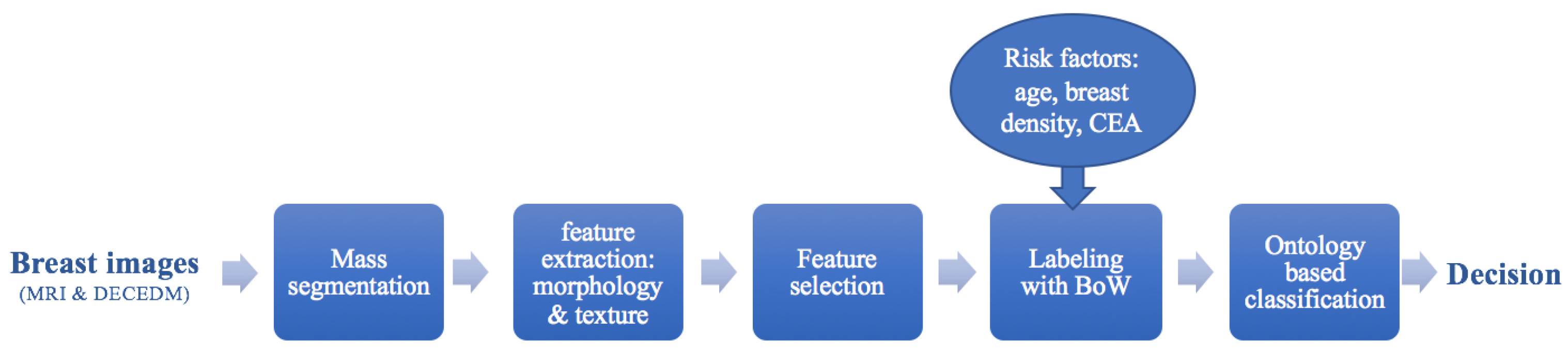
2. Material and Methods

An overview of the proposed breast cancer CAD system is illustrated in Figure 1. After the segmentation step, a set of morphological features are extracted to characterize the detected lesion. A feature selection process is then applied to discard irrelevant features extracted from MRI and DECEDM. Generally, knowledge-based systems (KBS) are used to solve complex problems which deal with a big amount of data. Unlike conventional computer programs, KBS represent high level knowledge explicitly using tools such as ontology. The new generations of KBS use a combination of structured representation of domain knowledge and reasoning tools of a particular domain. The semantic gap existing between low level image based features and clinical data on the one hand and expert concepts handled in analysis and diagnosis on the other hand needs to be filled by semantic annotation or labeling [16]. The modeled features are a subject to a data fusion with kinetic feature and risk factors in order to build a BoW. Different concepts defining our BoW are used including texture, shape, breast density, breast MRI and DECEDM contrast enhancement and patient age. In a further step, the modeled (BoWs) are used to classify the lesion severity as benign or malignant.

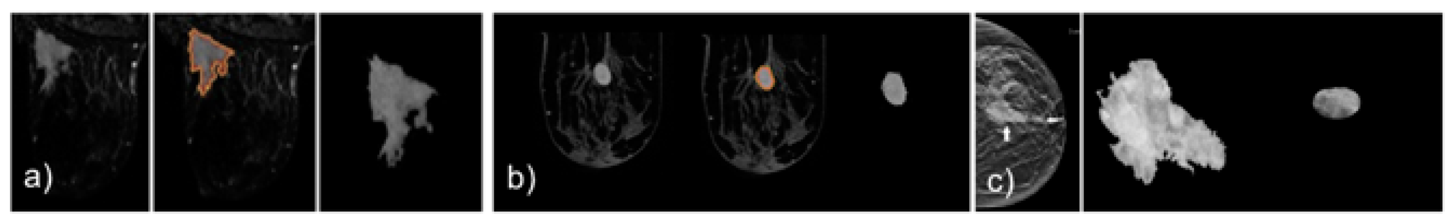
2.1. Mass Segmentation

Several image processing methods for breast lesion segmentation exist [17,18]: region growing is recommended and frequently used for image segmentation [6,19]. Nevertheless, it has a serious limitation since it requires a criterion of homogeneity. In case of a non-homogeneous area (case of malignant lesion), the similarity measure generates variations that can interrupt the growth process. Fuzzy C-means clustering (FCM) based segmentation can overcome this limitation in case of non homogeneous lesion. Indeed, it is widely used too to segment breast masses [20,21]. However, conventional FCM clustering is sensitive to noise and imaging artifacts since it does not integrate spatial context information. The level set algorithm has not such limitation. It allows us to segment images with non homogeneous objects with hidden contour [22,23]. Let be a curve $\mathsf{\Gamma }$ in movement in a region $\mathsf{\Omega }$ as the zero level of a function $\varphi$ of higher dimensional hyper-surface. The interface in movement at point x at the instant t is defined as:

$$\mathsf{\Gamma }(t)=\{(x,t)|\varphi (x,t)=0\},$$

(1)

where $\varphi$ is positive inside $\mathsf{\Omega }$, negative outside, and null on $\mathsf{\Gamma }$. Items of this interface moves towards normal (gradient $\nabla \varphi$) at a speed function F according to the following equation:

$$\frac{\partial \varphi }{\partial t}+F.\nabla \phi =0.$$

(2)

Only the normal component $FN$ of F account, $FN=F.\nabla \phi /|\nabla \phi |$, with $|\nabla \phi |$ is the euclidean norm, thus Equation (2) becomes:

$$\frac{\partial \varphi }{\partial t}+FN.\nabla \varphi =0.$$

(3)

Although re-initialization is able to maintain the regularity of the level set function (LSF), it may move the zero-level set away from the expected position. Thus, the re-initialization step is avoided in level set method. Several level set methods without re-initialization exist in the literature [24,25]. The most appropriate one to our case of study is the FCM based segmentation method proposed by Chaunming’s et al. [26]. It presents a general variational level set formulation based on a distance regularization term and an external energy term that drives the motion of the zero-level contour toward desired locations. Such a formulation is called distance regularized level set evolution (DRLSE). Chunming et al. apply the DRLSE formulation to an edge-based active contour model for image segmentation. It allows us to reduce significantly the number of iterations and computation time with relatively large time step while maintaining sufficient numerical accuracy in both full domain and narrow-band implementations. The FCM is maintained smooth and stable during the level set evolution by signing distance functions for their unique property |$\nabla \phi$|=1. Accordingly, we applied Chunming’s et al. algorithm to segment breast masses from MRI images and DECEDM. The segmentation results are validated by two radiologists from the Farabi radiology center in Sfax–Tunisia and Georges Pompidou European Hospital (HEGP). Figure 2 presents samples of mass segmentation using level set method. Then, a set of shape and texture features are extracted from both modalities and the selection process is applied.

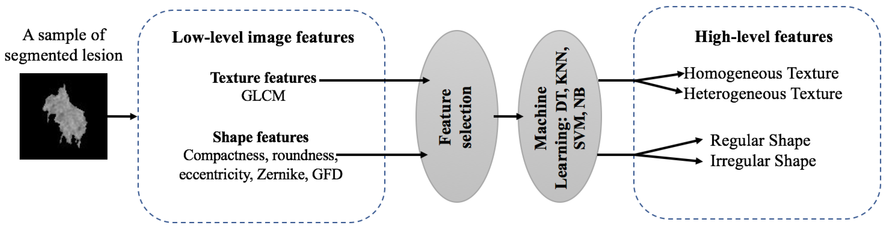
2.2. Feature Extraction

A texture analysis allows us to elaborate a description second order statistical distribution of gray levels in images. Gray level co-occurrence matrix (GLCM) represents how different pixel brightness values combinations occur in the image. Each value in GLCM matrix is considered to be the probability that a pixel with value i will be found adjacent to a pixel of value j given a certain distance d separating pixels and at a particular angle $\theta$ as defined below.

$$GLCM=\left(\begin{array}{c}p(1,1)\cdots p(1,N)\\ ⋮\ddots ⋮\\ p(N,1)\cdots p(N,N)\end{array}\right)$$

(4)

GLCM features are widely used in several different areas and in particular breast mass characterization [27,28,29]. According to Thibault et al. [28], GLCM offers an effective analysis of gray-level occurrences in the image at particular distance and/or orientation. Based on such statistical description, GLCM can yield an explicit formulation of texture heterogeneity and other texture features such as contrast Ct, correlation Cr, energy Eg, homogeneity Hg, entropy Ep, auto-correlation Ac, cluster prominence CP, cluster shade CS, dissimilarity Ds, maximum probability MP and variance Vr. In addition to GLCM features, we extracted local binary pattern features (LBP) and Histogram of Oriented Gradients (HOG) features from the segmented lesions. LBP features are widely used to describe image texture in different domains [30,31] and specially in medicine [32,33]. LBP features encode local texture information in order to be used for tasks such as classification, detection and recognition. The conventional LBP operator extracts information that is invariant to local grayscale variations in the input image. It is computed at each pixel location, taking into consideration the values of a small circular neighborhood (with radius R) around the value of a central pixel $q_c$. The LBP operator is defined as follows:

$$LBP(N,R)=\sum _{N=0}^{N-1}s(q_N-q_c)2^N,$$

(5)

where N is the number of pixels in the neighborhood, R is the radius, and $s(x)=1$ if x≥ 0, otherwise 0. Here the number of neighboors N is 8 and the radius R is 1.

The histogram of oriented gradients HOG is a feature descriptor used in computer vision and image processing for object detection and characterization [34,35]. The main idea of the histogram of oriented gradients descriptor is that an object and a shape within an image can be characterized by the distribution of intensity gradients or edge directions. The image was partitioned into small connected regions called cells, and for the pixels within each cell, a histogram of gradient directions was compiled. The features employed in this work are based on the HOG proposed by Dalal and Triggs [36]. The applied HOG function returned extracted HOG features from a grayscale input image in a $1byN$ vector, where N is the HOG feature length. The size of HOG cell and the number of cells in block are specified in pixels as a two-element vectors, here a [8 8] cell size and a [2 2] cells in block are applied. The number of orientation histogram bins is fixed to 9 and the orientation values are spaced from 0 through 180.

Such descriptors are used for lesion modelling.

Shape descriptors can be categorized into two groups: contour-based shape descriptors (compactness, eccentricity, Fourier descriptor, wavelet descriptors, shape signatures, etc.) and region-based shape descriptors (geometric moments, Zernike moments, generic Fourier descriptors (GFD), etc.). Contour-based shape techniques exploit only shape boundary information. In region-based techniques, all the pixels within a shape region are taken into account to get the shape representation. Shape features are very pertinent in breast cancer diagnosis [6,27,37,38]. A set of conventional shape features is extracted including compactness Cp, roundness Rd, eccentricity Ec, Zernike moments (ZM) and generic Fourier descriptors GFD.

• Compactness is used to quantify the connection between portions of a region. A highly non-convex lesion (malignant) have a high compactness index, whereas benign lesions have a low compactness value index.

  $$Compactness=4\pi .area/perimete{r}^2$$

  (6)
• Roundness is a measure of the similarity of an object shape to a circle. Shape with a roundness index closer to 1 indicates that the mass is approximately round so it is rather benign.

  $$Roundness=perimete{r}^2/4\pi .area$$

  (7)
• Eccentricity is the measure of aspect ratio of a region. It is defined by the ratio of the major axis to the minor axis. A shape with an eccentricity index too close to 1 is almost a circle.

  $$Eccentricity=MajorAxis/MinorAxis$$

  (8)
• Zernike moments are used as an object descriptor in several pattern recognition systems, edge detection and image retrieval applications with significant results. It allows us to represent image properties without redundancy and overlap of information between the moments thanks to complex kernel functions based on Zernike polynomials orthogonal to each other. The discrete form of the Zernike moments of an image size N × N is defined as follows:

  $$Z_{nm}=\frac{n+1}{{\lambda }_N}\sum _{x=0}^{N-1}\sum _{y=0}^{N-1}f(x,y)R_{nm}({\rho }_{xy})e^{-jm{\theta }_{xy}}$$

  (9)

  where $0\le {\rho }_{xy}\le 1$, and ${\lambda }_N$ is a normalization factor. The transformed distance ${\rho }_{xy}$ and the phase ${\theta }_{xy}$ at the pixel of (x,y) are given by:

  $${\rho }_{xy}=\frac{\sqrt{{(2x-N+1)}^2+{(N-1-2y)}^2}}{N},$$

  (10)

  $${\theta }_{xy}={tan}^{-1}(\frac{N-1-2y}{2x-N-1}).$$

  (11)
• GFD extracted from spectral domain by applying 2D Fourier transform on polar raster sampled shape image. It allows multi-resolution feature analysis in both radial and angular directions. The GFD, based on the polar Fourier (PF), is defined as:

  $$GFD(m,n)=\{\frac{|PF(0,0)|}{M_{11}},\frac{|PF(0,1)|}{PF(0,0)},\dots ,\frac{|PF(m,n)|}{PF(0,0)}\},$$

  (12)

  where m and n are the radial and angular frequencies and $M_{11}$ is the 1st order moment. Here we choose m= 4 and n= 9.

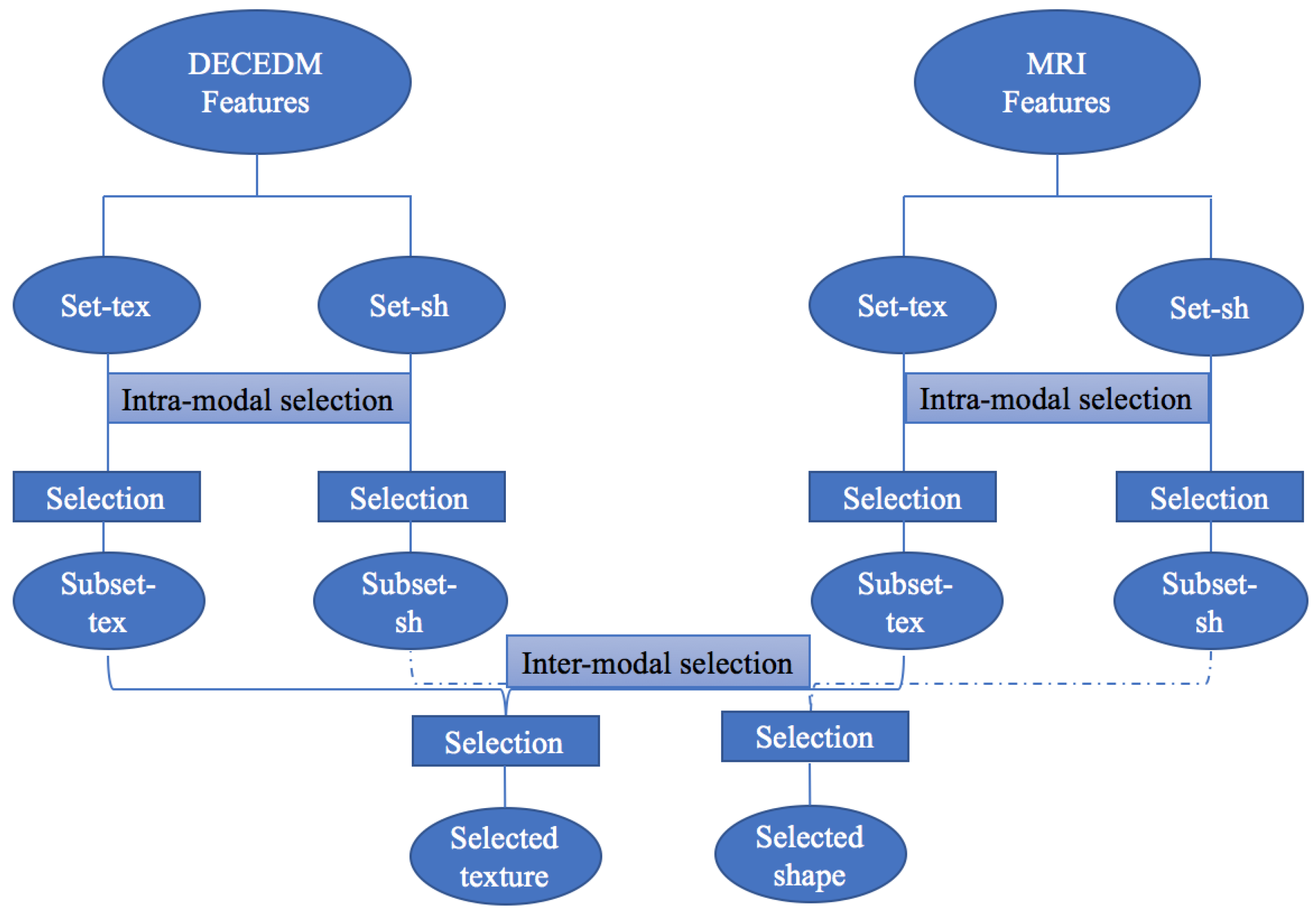
2.3. Feature Selection

Generally, feature selection methods are built independently. Their combination may lead to positive correlations since they aim to achieve the same goal and are based on the same learning data [39,40,41,42]. Several selection techniques can be used to keep only pertinent features and make decision more efficient [43,44,45,46]. Bagging, random subspace, random forest, adaBoost, and rotation forest methods have been applied for different applications [41,47,48,49] such as health-care and especially for breast cancer diagnosis [39,50,51,52,53,54]. Nonetheless, such approaches have some limits due to eventual correlation between descriptors. Besides, they often require a consistent amount of learning data to be efficient. Small databases could present an inherent risk of imprecision and under-fitting which presents a great challenge for many recognition systems. Here, we are in front of two main challenges: dealing with features extracted from two different modalities and dealing with a small sample set case. In such cases, researchers require the use of fuzzy integral since they are able to classify patterns in a non-dichotomous way and to handle vague information. Many fuzzy integral-based aggregation processes exist in the literature, and they can be divided into additive integrals such as simple weighted average (SWA) [55], quasi arithmetic means (QAM), ordered weighted average (OWA) [17,56], weighted min and weighted max, etc, and non-additive integrals such as Sugeno integral, Choquet integral, etc. Unfortunately, additive operators presume that attributes are always independent to each other. This assumption is inapt with real scenario where the features hold interactive characteristics [57]. Therefore, aggregation should not be always carried out using additive operators. According to Michel Grabisch [58], the OWA operator is a particular case of Choquet integral. Sugeno and Choquet integral operator could be used to deal with these interactive features. Although both integrals are able to capture the usual interactions existing between the features, the application of Choquet integral is widening across many disciplines with greater extent than the Sugeno integral. Firstly, according to Iourinski and Modave [59], Choquet integral is better suited for numerical or quantitative based problems, whereas, the Sugeno integral is more ideal for qualitative problems. In fact, the application of Choquet integral can generate more practical outcomes as most of the multiple feature problems involve numbers which have a real meaning (interval or ratio level of measurement) where cardinal aggregation is intended, unlike Sugeno integral which is more suitable for ordinal aggregation where only the order of the elements is important. Secondly, Choquet integral has the merit in producing unique solution in contrast to Sugeno integral [57]. According to a comparison study between Choquet and Sugeno integrals as aggregation operators for pattern recognition, done by Martinez and al. [60], the Choquet integral gives better results than the Sugeno integral using and without using the cross validation method. Accordingly, we based on the Choquet integral for breast cancer feature selection with a cross validation method. Inspired by expert’s reasoning, the proposed selection process scheme is dressed in Figure 3. As illustrated, a two level selection process is applied: an intra-modal selection where feature selection process concerns the different modalities involved in the analysis and an inter-modal selection where most relevant features extracted from one modality are selected. At the intra-modal selection level, each modality is treated separately. The selection process is applied on the whole set of texture and shape features denoted by Set-Tex and Set-Sh respectively. As result, the selected features constitute two subsets Subset-Tex and Subset-Sh of selected features. Then, an inter-modal selection is applied. The selected features are combined and the selection process is restarted. Finally, we get two subsets of selected features; selected texture features and selected shape ones.

2.3.1. Choquet Integral Selection

Fuzzy integrals showed a great performance to resolve the problem of limited database. They have been proposed by Sugeno for multi-criteria evaluation application [61]. A feature aggregator is applied since it takes the advantage of all the features used and takes into account the interactions between them. Generally, feature fusion is defined as follows; let m be the number of classes $C_1$,…, $C_m$ and n the number of features $F_1$,…, $F_n$. Given a new pattern $x_0$, we want to find to which class it does mostly belong. Here, we need firstly to compute for each feature j and each class i the confidence degree ${\varphi }_j^i$ which defines the following statement: “According to $F_j$, $x_0$ belongs to the class $C_i$”. Then all these partial confidence degrees are combined into a global one noted $\varphi (C_i|x)$ using a suitable aggregation operator H giving the statement “$x_0$ belongs to the class $C_i$”. The global confidence degree is then defined by:

$$\varphi (C_i|x)=H({\varphi }_1^i,\dots ,{\varphi }_n^i)$$

(13)

Finally, $x_0$ is assigned to the class for which the global confidence degree is the highest.

Choquet integral was first introduced in the capacity theory [62]. Gader et al. [41] show that Choquet integral gives better recognition results than other several popular methodologies. In addition to assigning a weight to each feature in the final decision, Choquet integral takes into consideration interactions between decision rules, while providing a model of a robust decision even in the presence of a small training data-set [63]. In fact, since all decision rules have the same aim, a synergy could occur among them. Choquet integral operators allow to assign a weight to each subset of decision rules by capturing its importance in the decision in an associated concept measure called capacity. Accordingly, feature importance index and feature interaction index are considered in selection. Features with lower importance and interaction indexes are discarded. Applying an appropriate heuristic algorithm such as Grabisch algorithm allows us to have a good learning of the fuzzy measure even if only few training data are available [64]. Choquet integral of a set of confidence degrees $\overrightarrow{\varphi }={[{\varphi }_1\dots {\varphi }_n]}^t$ noted $C_{\mu }(\overrightarrow{\varphi })$ is defined by:

$$C_{\mu }(\overrightarrow{\varphi })=\sum _{j=1}^n{\varphi }_{(j)}\left[\mu (F_{(j)})-\mu (F_{(j+1)})\right]$$

(14)

where $\mu$ is a fuzzy measure on X and $F_{(j)=1,\dots ,n}$ represents n associated features in increasing order and $A_{(n+1)}=\varnothing$. Choquet integral is based on two main steps: a learning step where a confusion measure is computed and the extraction step where only the most pertinent decision rules are kept.

2.3.2. Learning Step

Choquet integral is an aggregation operator that relies on the definition of an adequate fuzzy measure called capacity. In case of lack of expert information, this capacity is learned from the training set. The fuzzy measure is determined by minimizing the error existing between the learned value by Choquet integral and the expected evaluation. Generally, such a problem is solved using the Lemke method. Nevertheless, such a method requires a huge amount of learning data. To overcome such a problem, heuristic algorithms are developed. Their aim is to find out an approximation of the fuzzy measure to minimize the criterion error. Grabisch [63] proposed an approach based on a gradient algorithm. It is assumed that in case of lack of information, the most reasonable way of aggregation is the arithmetic mean. According to Grabisch, a fuzzy measure is represented by a lattice of 2${}^n$ coefficients to keep the monotonicity of the integral. The 2${}^n$ coefficients presents the measures of the 2${}^n$ subsets of X. Grabisch opted for a lattice representation to perform the fuzzy measures. The 2${}^n$ coefficients defining the fuzzy measure are arranged in a lattice with the usual ordering on real numbers, the same as the Boolean lattice of subsets of X, ordered with inclusion. Each node of the lattice represents the fuzzy measure associated to a particular subset of X. Let be a sample of a lattice when n = 4 for a set of features X = {$x_1$, $x_2$, $x_3$, $x_4$}. Knowing that ${\mu }_{23}$ denotes $\mu$({x${}_2$, x${}_3$}). The lattice has $n+1$ horizontal layers or nodes related by links, ordered from 0 (for ${\mu }_{\varnothing }$) to n (for ${\mu }_X$). A path is a sequence of links starting from the node ${\mu }_{\varnothing }$ and arriving to the node ${\mu }_X$. For a given node in layer l, its upper neighbors (resp. lower neighbors) are the set of nodes in the layer l + 1 (resp. $l-1$) linked to it. Considering an input vector of partial confidence degrees $\varphi$ = (${\varphi }_1$, ${\varphi }_2$, ${\varphi }_3$, ${\varphi }_4$) with ${\varphi }_1\le {\varphi }_2\le {\varphi }_3\le {\varphi }_4$. Applying the Choquet integral for $\varphi$ involves only the fuzzy measures along one path in lattice according to the ordering of the ${\varphi }_I$ which implies the nodes ${\mu }_0$, ${\mu }_3$, ${\mu }_{23}$, ${\mu }_{234}$, ${\mu }_{1234}$. For a learning data set (x,y) where x is the input and y is the output, we need to find for Choquet integral the best fuzzy measure $\mu$ which allows us to minimize the sum of squared errors between the model and the system. Therefore, we have to take into consideration four major points: firstly, the fuzzy measure monotonicity constraints. Secondly, all the coefficients situated on a path from ∅ to X must be used respecting the order of the values of ${\varphi }_1$,…, ${\varphi }_n$. The third point is about having too few data to use. In such a case, some coefficients of the lattice are not used, then they cannot be modified by some gradient considerations. Finally, in the absence of any learning data and any information, the only reasonable solution seems to be to choose the average value of the input $\frac{1}{n}{\sum }_i{x}_i$ i.e., $\mu$($\{x_i\})$= $1/n$, for all i [63], in the lattice representation this corresponds to a state where every node in a layer l is equidistant from its upper $(l+1)$ and lower $(l-1)$ neighbors.

The fuzzy measure is initialized to the weighted mean and the weights are learned from the training set. In fact, for each feature $F_i$ of the learning set, let $r_i$ $(1\le i\le n)$ be its recognition rate. A feature with a higher recognition rate is supposed more important and the weight associated to it is defined as:

$${\omega }_i=r_i/\sum _{j=1}^n{r}_j$$

(15)

with

$$\sum _{i=1}^n{\omega }_i=1.$$

(16)

2.3.3. Extraction Step

The importance index (or Shapley index) characterizes the importance of each feature in the final decision. It is based on the definition proposed by Shapley [65] in the game theory and introduced in a fuzzy measure context by Murofushi and Soneda [66]. For a fuzzy measure $\mu$ and a feature $F_i$, the importance index is defined as follows:

$$I_S(\mu ,F_i)=\frac{1}{n}\sum _{t=0}^{n-1}\frac{1}{\left(\begin{array}{c}n-1\\ t\end{array}\right)}\sum _{T\subseteq N\setminus F_i,|T|=t}\left[\mu (T\cup F_i)-\mu (T)\right].$$

(17)

The importance index is interpreted as an average value of the marginal contribution $\mu (T\cup F_i)-\mu (T)$ of the feature i alone in all combinations. The sum of the indexes of all features is equal to 1, i.e., ${\sum }_{i=1}^n{I}_S(\mu ,F_i)=1$. A feature with an importance index value less than $1/n$ has a low impact on the final decision. Otherwise an importance index greater than $1/n$ characterizes an attribute which is more important than the average.

The interaction index or Murofushi and Soneda index [66,67] allows us to evaluate the degree of interaction between two features. If the fuzzy measure is non-additive, some features interact. The assessment of the interaction index of $F_i$ and $F_j$, is defined by:

$$I_I(\mu ,F_i{F}_j)=\sum _{T\subseteq X\setminus F_i{F}_j}\frac{(n-t-2)!t!}{(n-1)!}({\mathsf{\Delta }}_{F_i{F}_j\mu })(T).$$

(18)

A positive interaction index for two features i and j means that the importance of one feature is strengthened by the second. Thus, both features are complementary and their combination improves the final decision. The importance of this complementarity is given by the value of the interaction index. A negative interaction index indicates that the sources are antagonist, and their combination is worst than the case where each feature is applied alone.

At each level of the selection process, the feature (features) having the lowest weight and positively interacts the least with other features, is considered to be the weakest and to blur the final decision. Then, it is (they are) discarded. A two-step selection scheme is implemented to discard these features. Firstly, a feature with an importance index higher than $1/n$ has a higher importance in the final decision. The set noted $M_S$ of least significant features having the lowest importance index (less than $1/n$), is selected:

$$M_S=\{F|I_S(\mu ,F)<1/n\}.$$

(19)

Then, we remove from $M_S$ the subset of features having the least positive synergy with the others. In fact, the values of the interaction indexes of each feature from the subset $M_S$ are averaged to estimate its global interaction. The feature or the subset of features to be removed from $M_S$, noted $M{M}_S$, is composed of the features which have the lowest global interaction index. $M{M}_S$ is defined as follows:

$$M{M}_S=\{F|min\sum _{j=1,n}|I_I(\mu ,F_j){|\}}_{k\in M_S}$$

(20)

where the global mean interaction index is defined by

$$\frac{1}{|M_S|}\sum _{F\in M_S}\sum _{j=1,n}{I}_j(\mu ,F_j).$$

(21)

The feature (features) having the lowest index value is discarded. The selection process stops once we get a steady correct classification rate, when the kept features have an importance index higher than $1/n$, or when we get less than three features to classify.

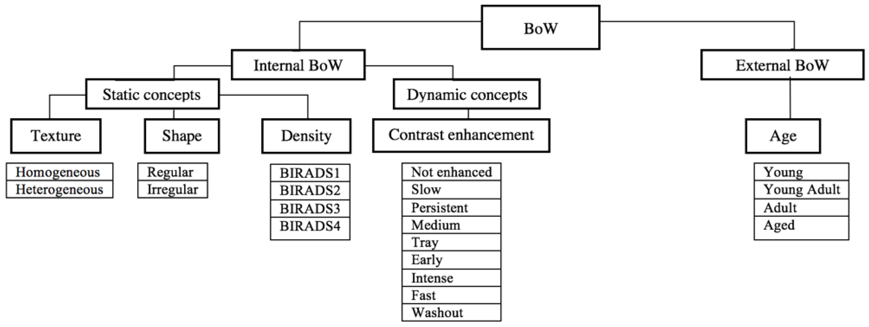
2.4. Bag of Words Modeling

Here, we derive the different concepts which define our BoW. Figure 4 illustrates these concepts. They could be divided into internal image derived BoWs such as static knowledge (shape, texture, breast density) and dynamic knowledge (breast MRI and DECEDM contrast enhancement agent CEA), and external BoWs or meta-knowledge such as the age. Known that breast density and contrast enhancement are extracted from patient file, shape and texture features are modeled by labeling the low level extracted features from images. Accordingly, we use here two texture labels to characterize breast masses: heterogeneous and homogeneous, and two shape labels: regular for oval and round shapes or irregular for other ones. Breast density characterizes the breast tissue fatness and homogeneity. Higher breast density induces low contrast in mammography making breast cancer detection harder. According to the breast imaging reporting and data system (BIRADS), semantic of the ACR (American College of Radiology), breast density can be classified into four groups where the risk of missing cancer detection increases from category 1 to category 4. The perception of the CEA in breast MRI and DECEDM can give an idea about the lesion type: no enhancement in DECEDM or slow and persistent in MRI for benign lesion, medium and tray enhancement in MRI for intermediate and intense enhancement in DECEDM or early, fast and washout enhancement in MRI for malignant lesion. Age is modulated by age range (young for age < 25, adult young for 25 ≤ age < 50, adult for 50 ≤ age < 75 and aged for age ≥ 75).

2.5. Image Annotation

Here, we are based on texture and shape features for image annotation. A set of texture features and shape descriptors are computed from the segmented lesions from both breast MRI and DECEDM. A set of well-known classifiers including decision tree (DT), K-nearest neighbors (KNN), support vector machine (SVM) and naive Bayes (NB) were used and compared to find the most appropriate one giving an adequate description of the correspondent set of low level features for each modality (MRI and DECEDM) and for each type of feature. For the training step using SVM, an optimization method was used to identify support vectors $s_i$, weights ${\alpha }_i$, and bias b that were used to classify vectors x according to the following equation:

$$c=\sum _i{\alpha }_{i}k(s_i,x)+b,$$

(22)

where k is a kernel function. Here we choose, by default, a linear function. If c≤ 0, then x is classified as a member of the first group, otherwise it is classified as a member of the second group. The method used to find the separating hyperplane is sequential minimal optimization (SMO). For the classification step, we used results from the training to classify vectors x according to the same Equation (22). A binary regression decision tree was used when applied DT classifier. Using the KNN method, the euclidean distance is applied and the samples are classified using the nearest method where the majority rule with nearest point tie-break is applied. To train a multi-class naïve bayes model, we use predictors and class labels. The predictor distribution within each class is modeled using a Gaussian distribution.

Once the selection process was achieved, texture features were combined using a classifier. Benign lesions have a homogeneous texture, whereas, malignant ones are rather heterogeneous (more vascularized). As well as texture feature, selected shape features are combined using a classifier. Two different mass shapes can be identified: regular for benign masses and irregular for malignant ones (Figure 5).

3. Results and Discussion

3.1. Database

An appropriate DECEDM and MRI private database built with collaboration with the radiology department of the European Hospital Georges–Pompidou (HEGP), containing a set of breast screenings from 2014 to 2015 for high risk patients, is used in this study. The age range of patients is between 26 and 80 years. The MRI database consists of 58 mass lesions from 40 patients. Of the lesions, 14 were identified as benign and 44 others as malignant. Only three of the 14 benign lesions and 27 of the 44 malignant lesions are detected on DECEDM rather because they are too small, or not well vascularized. The corresponding physical lesions on both modalities were identified visually by an expert radiologist based on visual criteria and biopsy-proven reports. The data are not publicly available due to them containing information that could compromise research participant privacy or consent.

3.2. Feature Selection

In our case of study, breast masses were divided into two classes: benign lesions B and malignant lesions M. For each modality (MRI and DECEDM) and for each set of features (texture and shape), each lesion l of the training set was described by the couple $({\varphi }^B,{\varphi }^M)(l)$ where ${\varphi }^B$ is the confidence degree that a lesion l belongs to class benign and ${\varphi }^M$ is the confidence degree that a lesion l belongs to class malignant. For example, in MRI (resp. DECEDM), each lesion was characterized by a set of texture features and shape features. Then, we got two couples ${({\varphi }^B,{\varphi }^M)}_{texture}(l)$ and ${({\varphi }^B,{\varphi }^M)}_{shape}(l)$ corresponding to texture and shape features.

Table 1. A sample of global confidence degrees for benign and malignant classes of 13 lesions obtained when applying Choquet integral on dual energy contrast enhancement mammography (DECEDM) texture features. Correct recognition rate here is 85%.

Lesion	${\mathit{\varphi }}^{\mathit{B}}$	${\mathit{\varphi }}^{\mathit{M}}$	Class
L1	0.76	0.61	B
L2	0.61	0.82	M
L3	0.74	0.72	B
L4	0.62	0.62	M
L5	0.58	0.63	M
L6	0.79	0.67	B
L7	0.49	0.79	M
L8	0.54	0.82	M
L9	0.63	0.76	M
L10	0.66	0.82	M
L11	0.54	0.80	M
L12	0.54	0.81	M
L13	0.57	0.81	M

shows a sample of global confidence degrees when applying Choquet integral on partial confidence degrees of DECEDM texture features. The analysis of Choquet lattice attributes to each feature a score based on its Shapley index and its global interaction index. A sample of Shapley and interaction indexes is provided in

Table 2. A sample of Shapley values of DECEDM texture features.

Shapley Values
Cr	Ep	MP	Ds	Hg	Eg	CS	Vr	CP	Ac	HOG	LBP	Ct	13 features
0.069	0.072	0.072	0.076	0.076	0.076	0.076	0.077	0.077	0.079	0.079	0.080	0.090	0.077

and

Table 3. A sample of interaction indexes of DECEDM texture features.

Interaction Values
	Ct	Cr	Eg	Hg	Ep	Ac	CP	CS	Ds	MP	Vr
Ct	-	7.56× 10${}^{-4}$	−1.42× 10${}^{-4}$	−2.19× 10${}^{-3}$	−7.37× 10${}^{-4}$	1.24× 10${}^{-3}$	−2.96× 10${}^{-4}$	−1.19× 10${}^{-3}$	3.03× 10${}^{-4}$	7.60× 10${}^{-4}$	1.91× 10${}^{-3}$
Cr	7.56× 10${}^{-4}$	-	1.49× 10${}^{-3}$	4.69× 10${}^{-4}$	1.93× 10${}^{-4}$	−5.29× 10${}^{-4}$	−2.17× 10${}^{-3}$	−1.12× 10${}^{-3}$	1.67× 10${}^{-3}$	1.25× 10${}^{-3}$	7.51× 10${}^{-5}$
Eg	−1.42× 10${}^{-4}$	1.49× 10${}^{-3}$	-	−2.80× 10${}^{-3}$	−1.26× 10${}^{-3}$	−5.78× 10${}^{-4}$	−2.14× 10${}^{-3}$	−8.45× 10${}^{-4}$	7.90× 10${}^{-4}$	−2.55× 10${}^{-4}$	3.30× 10${}^{-4}$
Hg	−2.19× 10${}^{-3}$	4.69× 10${}^{-4}$	−2.80× 10${}^{-3}$	-	3.88× 10${}^{-4}$	1.16× 10${}^{-3}$	−1.42× 10${}^{-4}$	−1.48× 10${}^{-3}$	1.15× 10${}^{-4}$	7.51× 10${}^{-4}$	1.81× 10${}^{-3}$
Ep	−7.37× 10${}^{-4}$	1.93× 10${}^{-4}$	−1.26× 10${}^{-3}$	3.88× 10${}^{-4}$	-	2.09× 10${}^{-3}$	4.43× 10${}^{-4}$	4.06× 10${}^{-3}$	−1.54× 10${}^{-3}$	−1.89× 10${}^{-3}$	−2.43× 10${}^{-3}$
Ac	1.24× 10${}^{-3}$	−5.29× 10${}^{-4}$	−5.78× 10${}^{-4}$	1.16× 10${}^{-3}$	2.09× 10${}^{-3}$	-	−1.97× 10${}^{-3}$	−2.24× 10${}^{-3}$	−1.52× 10${}^{-3}$	2.08× 10${}^{-4}$	−1.94× 10${}^{-4}$
CP	−2.96× 10${}^{-4}$	−2.17× 10${}^{-3}$	−2.14× 10${}^{-3}$	−1.42× 10${}^{-4}$	4.43× 10${}^{-4}$	−1.97× 10${}^{-3}$	-	5.93× 10${}^{-4}$	2.27× 10${}^{-3}$	1.32× 10${}^{-3}$	5.83× 10${}^{-4}$
CS	−1.19× 10${}^{-3}$	−1.12× 10${}^{-3}$	−8.45× 10${}^{-4}$	−1.48× 10${}^{-3}$	4.06× 10${}^{-3}$	−2.24× 10${}^{-3}$	5.93× 10${}^{-4}$	-	4.50× 10${}^{-3}$	2.95× 10${}^{-3}$	2.90× 10${}^{-3}$
Ds	3.03× 10${}^{-4}$	1.67× 10${}^{-3}$	7.90× 10${}^{-4}$	1.15× 10${}^{-4}$	−1.54× 10${}^{-3}$	−1.52× 10${}^{-3}$	2.27× 10${}^{-3}$	4.50× 10${}^{-3}$	-	−2.11× 10${}^{-3}$	−1.55× 10${}^{-3}$
MP	7.60× 10${}^{-4}$	1.25× 10${}^{-3}$	−2.55× 10${}^{-4}$	7.51× 10${}^{-4}$	−1.89× 10${}^{-3}$	2.08× 10${}^{-4}$	1.32× 10${}^{-3}$	2.95× 10${}^{-3}$	−2.11× 10${}^{-3}$	-	−1.89× 10${}^{-3}$
Vr	1.91× 10${}^{-3}$	7.51× 10${}^{-5}$	3.30× 10${}^{-4}$	1.81× 10${}^{-3}$	−2.43× 10${}^{-3}$	−1.94× 10${}^{-4}$	5.83× 10${}^{-4}$	2.90× 10${}^{-3}$	−1.55× 10${}^{-3}$	−1.89× 10${}^{-3}$	-
LBP	8.31× 10${}^{-5}$	−5.73× 10${}^{-4}$	2.82× 10${}^{-3}$	1.38× 10${}^{-3}$	5.76× 10${}^{-4}$	1.16× 10${}^{-3}$	7.44× 10${}^{-4}$	−3.78× 10${}^{-3}$	−1.57× 10${}^{-3}$	−1.82× 10${}^{-3}$	−1.18× 10${}^{-3}$
HOG	−5.02× 10${}^{-4}$	−1.50× 10${}^{-3}$	2.59× 10${}^{-3}$	5.43× 10${}^{-4}$	1.06× 10${}^{-4}$	1.18× 10${}^{-3}$	7.69× 10${}^{-4}$	−4.35× 10${}^{-3}$	−1.35× 10${}^{-3}$	7.12× 10${}^{-4}$	−3.71× 10${}^{-4}$
	LBP	HOG
Ct	8.31× 10${}^{-5}$	−5.02× 10${}^{-4}$
Cr	−5.73× 10${}^{-4}$	−1.50× 10${}^{-3}$
Eg	2.82× 10${}^{-3}$	2.59× 10${}^{-3}$
Hg	1.38× 10${}^{-3}$	5.43× 10${}^{-4}$
Ep	5.76× 10${}^{-4}$	1.06× 10${}^{-4}$
Ac	1.16× 10${}^{-3}$	1.18× 10${}^{-3}$
CP	7.44× 10${}^{-4}$	7.69× 10${}^{-4}$
CS	−3.78× 10${}^{-3}$	−4.35× 10${}^{-3}$
Ds	−1.57× 10${}^{-3}$	−1.35× 10${}^{-3}$
MP	−1.82× 10${}^{-3}$	7.12× 10${}^{-4}$
Vr	−1.18× 10${}^{-3}$	−3.71× 10${}^{-4}$
LBP	-	2.17× 10${}^{-3}$
HOG	2.17× 10${}^{-3}$	-

for DECEDM texture features. In this sample, the selection process is applied on DECEDM texture features extracted from 13 lesions. Capacities were learned from the test samples and their different combinations are built based on Grabisch algorithm. Then, based on the learned capacities, global interaction indexes ${\varphi }^B$ and ${\varphi }^M$ are computed for each lesion (Table 1). Based on the ground truth, the correct classification rate was calculated by dividing the number of well classified lesion by the number of learning lesions. Here, a rate of 0.85% is obtained. DECEDM texture features were ordered in increasing order according to their importance indexes (Table 2). Features having an importance index higher than 0.077 (1/n; n = 13) are supposed to be pertinent. Then, interaction indexes were computed (Table 3). Feature having the lowest importance index and the lowest global interaction one is discarded. Here correlation had the lowest importance index of 0.069 and the lowest global interaction index of 9.9 × 10${}^{-10}$, then it is discarded.

At iteration epoch, the less relevant feature is discarded and the new correct classification rates are computed. Many criteria are used to evaluate the behavior of features. Here we use the recognition rate, i.e., the ratio between the number of samples rightly classified divided by the number of learning samples.

3.3. A Comparison between Choquet Intagral for Feature Selection and Other Selection Method

Before proceeding to the hierarchical selection, we aim to prove the effectiveness of using fuzzy integrals and specially Choquet integral for feature selection toward conventional feature selection methods, in case where a small database is available. Ververidis et al. [68] investigated a subset feature selection performed by the sequential floating forward selection (SFFS) with the Bayes classifier applied to speech emotion recognition. They assume that features obey the multivariate Gaussian distribution. Training and test sets are chosen by applying a cross-validation. The authors developed five feature selection algorithms including sequential forward selection (SFS), SFFS, sequential backward selection (SBS) and sequential floating backward selection (SFBS). Such selection algorithms are basically the most used in our domain and giving very satisfying selection and classification results. Based on the feature selection algorithms developed by Ververidis and Kotropoulos, we compare the selection results obtained when applying the already cited methods and our proposed algorithm on our dataset.

Table 4. Correct classification rates correct recognition rate (CCR) when applying sequential forward selection (SFS), sequential floating forward selection (SFFS), sequential backward selection (SBS), sequential floating backward selection (SFBS) and Choquet integral based selection.

Selection Method	CCR
SFS	0.92
SFFS	0.93
SBS	0.89
SFBS	0.86
Choquet	0.99

shows the correct classification rates when using each selection method.

The four sequential algorithms give satisfying correct classification rates even though we are dealing with a small database. Forward selection methods (SFS and SFFS) work better with 0.92 and 0.93 of correct recognition rate (CCR) respectively than backward selection methods (SBS and SFBS) with 0.89 and 0.86 respectively, and they are faster, which is expected, as forward methods start with small subsets and enlarge them while the backward methods start with large subsets and shrink them. Our selection algorithm based on Choquet integral outperforms the sequential algorithms with a CCR of 0.96. It is worth mentioning that according to the literature and our study that there is not a selection algorithm better than another for all cases, but the performance of each algorithm depends on the study case, the type of data and the database size. Nevertheless, we cannot deny the contribution of fuzzy integrals, namely the study of interactions between features and handling few data.

3.3.1. Structural Selection

The selection process was applied, in a first step, independently for each modality and each set of features (texture and shape). The following tables (

Table 5. Intra-modal selection of texture features. Correct classification rates obtained when applying the proposed selection process on breast MRI texture features. Ite: iteration. N: number of features kept. F: features. CCR: correct recognition rate.

Ite	N	F													CCR
		Ct	Cr	Eg	Hg	Ep	Ac	CP	CS	Ds	MP	Vr	LBP	HOG
1	13														0.85
1	12			X											0.85
2	11			X							X				0.85
3	10			X		X					X				0.85
4	9			X		X	X				X				0.85
5	8		X	X		X	X				X				0.85
6	7		X	X		X	X	X			X				0.92
7	6		X	X		X	X	X	X		X				0.92
8	5		X	X		X	X	X	X		X	X			0.92
9	4		X	X		X	X	X	X	X	X	X			0.92

,

Table 6. Intra-modal selection of shape features. Correct classification rates obtained when applying selection process on breast MRI shape features. Ite: iteration. N: number of features kept. F: features. CCR: correct recognition rate.

Ite	N	F					CCR
		Rd	Cp	Ec	ZM	GFD
1	5						0.92
2	4				X		0.92
3	2	X	X		X		0.92

,

Table 7. Intra-modal selection of texture features. Correct classification rates obtained when applying the proposed selection process on DECEDM texture features. Ite: iteration. N: number of features kept. F: features. CCR: correct recognition rate.

Ite	N	F													CCR
		Ct	Cr	Eg	Hg	Ep	Ac	CP	CS	Ds	MP	Vr	LBP	HOG
1	13														0.85
1	12		X												0.85
2	11		X			X									0.85
3	10		X			X					X				0.85
4	9		X	X		X					X				0.85
5	8		X	X		X				X	X				0.85
6	7		X	X	X	X				X	X				0.92
7	6		X	X	X	X			X	X	X				0.92
8	5		X	X	X	X			X	X	X	X			0.92
9	4		X	X	X	X		X	X	X	X	X			0.92

and

Table 8. Intra-modal selection. Correct classification rates obtained when applying selection process on DECEDM shape features. Ite: iteration. N: number of features kept. F: features. CCR: correct recognition rate.

Ite	N	F					CCR
		Rd	Cp	Ec	ZM	GFD
1	5						0.92
2	4				X		0.92
3	2	X	X	X	X		0.92

) show the evolution of correct classification rates when discarding at each iteration, the non relevant features, with the lowest Shapley index and the lowest interaction index.

The initial recognition rate obtained when using the combination of texture features of breast MRI is 0.85 (Table 5). Based on their importance and interaction indexes and the evolution of Choquet integral at each iteration of the selection process, irrelevant features are discarded. The most pertinent MRI texture features and which interact the best between them are: contrast, homogeneity, LBP and HOG features, leading to a CCR of 0.92.

According to Table 6, the initial CCR is steady (0.92) during the selection process. there is a reduction of features of 40%. According to their importance and interaction indexes, the most relevant MRI shape features are: eccentricity and GFD. According to this table, it is useless to add the remaining shape features in characterization.

Table 7 shows the evolution of the CCR from 0.85 to 0.92 when applying the selection process on DECEDM texture features. Based on their importance and interaction indexes a reduction of 69% of features is obtained. The most pertinent DECEDM texture features and which interact the best between them are: contrast, auto-correlation, LBP, HOG features and contrast.

Among the DECEDM extracted shape features, only GFD is kept since it outperforms other shape features. The recognition rate is steady during the selection process (Table 8), but a reduction of feature number of 40% is obtained.

3.3.2. Inter-Modal Selection

Once the most pertinent texture features of each modality are extracted, they are combined and the selection process is relaunched (

Table 9. Inter-modal selection. Correct classification rates obtained when applying the proposed selection process on breast MRI and DECEDM selected texture features. Ite: iteration. N: number of features kept. F: features. CCR: correct recognition rate.

Ite	N	F								CCR
		Ct1	Hg1	LBP1	HOG1	Ct2	Ac2	LBP2	HOG2
1	8									0.92
2	6	X				X				0.92
3	5	X				X	X			0.92

and

Table 10. Shapley values and interaction indexes obtained when applying the first iteration of the selection process on breast MRI and DECEDM selected texture features.

Shapley Values
Ite	Ct1	Hg1	LBP1	HOG1	Ct2	Ac2	LBP2	HOG2	1/N
1	0.121	0.127	0.130	0.129	0.121	0.122	0.125	0.125	0.125
2	-	0.165	0.171	0.171	-	0.160	0.166	0.167	0.167
3	-	0.200	0.200	0.200	-	-	0.200	0.200	0.200

). According to their importance indexes (Table 10) and interaction indexes, MRI contrast (Ct1) and DECEDM contrast (Ct2) have the lowest importance index of 0.121 (<1/n with $n=8$) and the lowest interaction index (≈0). Then, they are discarded and the selection process is relaunched. At the second iteration, DECEDM auto-correlation (Ac2) has the lowest importance index of 0.160 (<1/n with $n=6$) and the lowest interaction index, then it is discarded. At the third iteration of the selection algorithm, all texture features have a good Shapley value (≈1/n with $n=5$). Then, the selection process stops. The last 5 texture features are used to define our texture bag of words.

The three kept shape features extracted from MRI and DECEDM are used to define our shape bag of words since when applying Choquet integral they give a good recognition rate of 1. It is worth to mention that MRI GFD and DECEDM GFD outperform MRI eccentricity with a higher importance of 0.342 against 0.316 (≈1/n with $n=3$) to eccentricity.

3.4. Labeling Results

Semantic annotation is achieved using a classifier in order to be combined with other semantic concepts to build our BoW. This BoW is used to classify lesions into benign or malignant. To make a good choice, a set of classifiers are tested.

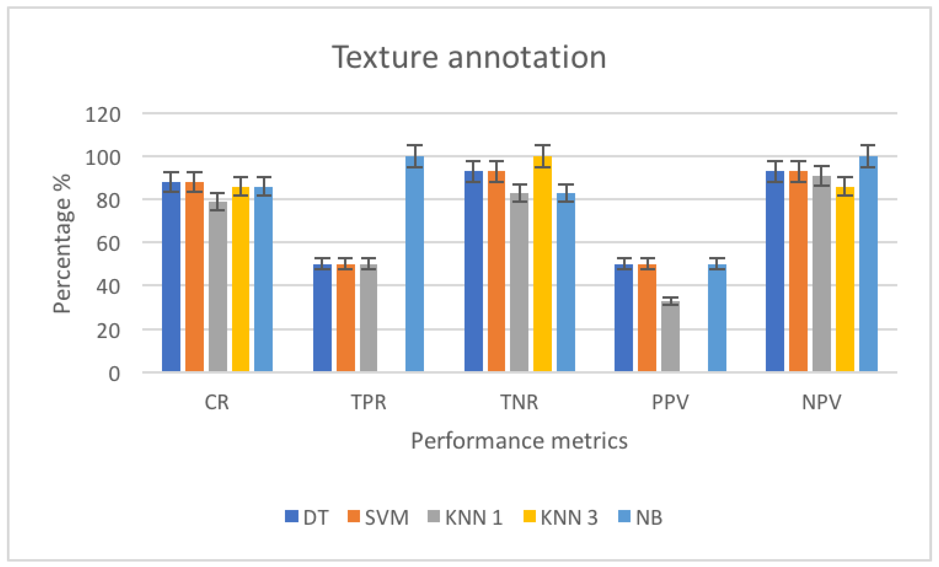
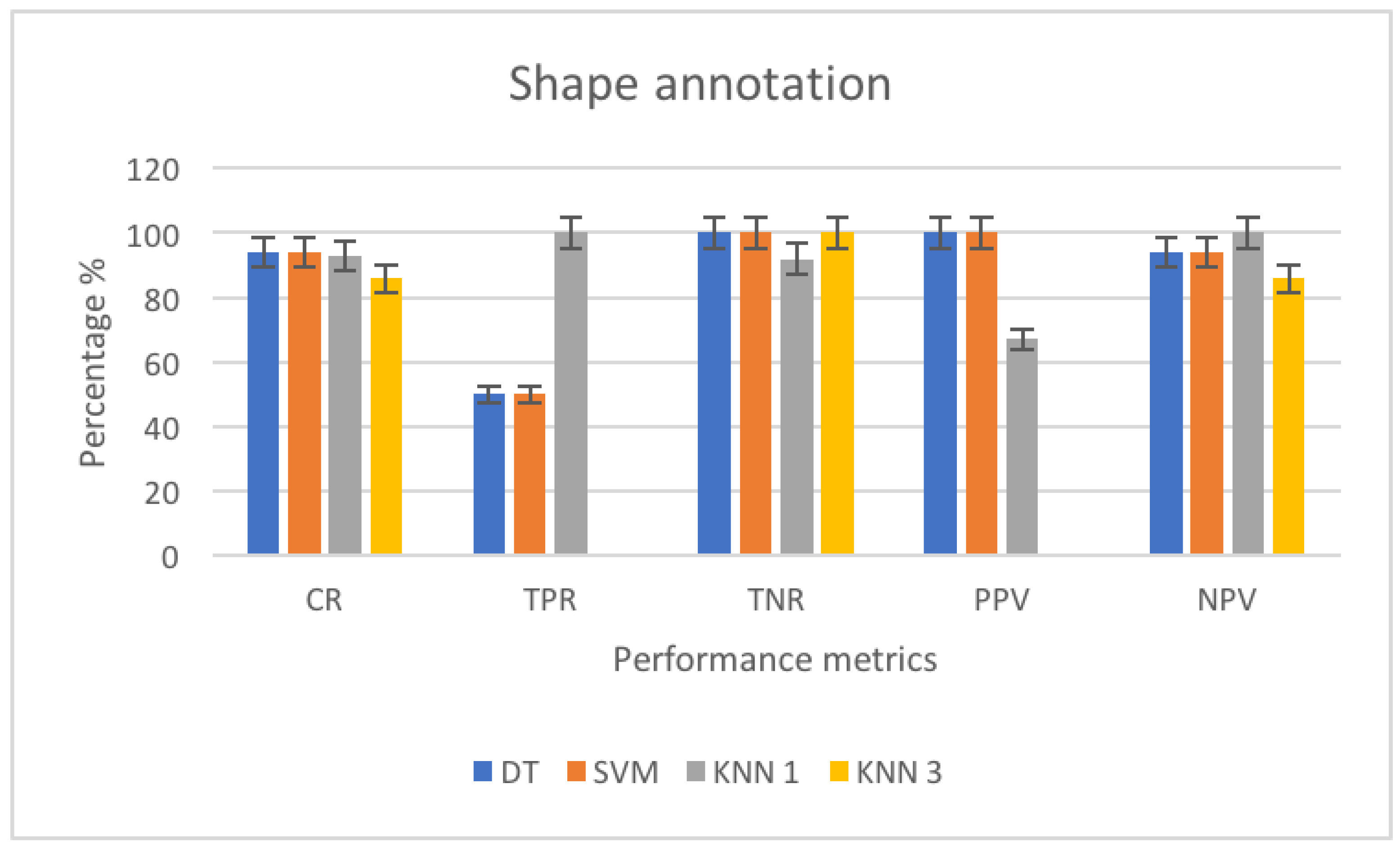
3.4.1. Performance Metrics

To evaluate the performance of our system, a set of metrics are deduced which are the area under the receiver operating characteristics (ROC) curve (AUC), the correct recognition rate (CCR), sensitivity, specificity, positive predictive value (PPV) and negative predictive value (NPV). Performance metrics are calculated from the confusion matrix also known as error matrix. The matrix columns represent the instance belonging to a predicted class. While matrix rows represent the instances of an actual class (or vice versa). the AUC is a measure of efficiency of features in discriminating classes. The CCR is the rate of the correctly classified samples, it is defined by:

$$\mathrm{CCR}=(\mathrm{correctly}\mathrm{classified}\mathrm{samples})/(\mathrm{Total}\mathrm{number}\mathrm{of}\mathrm{elements}).$$

(23)

Sensitivity or true positive rate (TPR) presents the correctly classified positive samples, it is defined as:

$$\mathrm{Sensitivity}=\mathrm{TPR}=\mathrm{TP}/(\mathrm{TP}+\mathrm{FN}).$$

(24)

Specificity or true negative rate (TNR) presents the correctly classified negative samples, its mathematical formula is:

$$\mathrm{Specificity}=\mathrm{TNR}=\mathrm{TN}/(\mathrm{TN}+\mathrm{FP}).$$

(25)

Precision, or PPV, presents the correctly classified positive samples, it is defined as follows:

$$\mathrm{Precision}=\mathrm{PPV}=\mathrm{TP}/(\mathrm{TP}+\mathrm{FP}).$$

(26)

NPV presents the correctly classified negative samples, its mathematical formula is as follows:

$$\mathrm{NPV}=\mathrm{TN}/(\mathrm{TN}+\mathrm{FN}),$$

(27)

where, TP are true positives (correct malignant prediction), FP are False Positives (incorrect malignant prediction), FN are False Negatives (incorrect benign prediction) and TN are True negatives (correct benign prediction).

3.4.2. Texture Annotation

Decision Tree and SVM outperform other classifiers to determine the texture related bag of words with an AUC of 1, a good correct classification rate (CCR = 88%), a good sensitivity (TPR = 50%), a good specificity (TNR= 93%), an acceptable positive predictive value (PPV = 50%) and high negative predictive value (NPV = 93%). KNN (for K = 1 and K = 3 successively) and NB are less efficient with an AUC of 0.88, 0.92 and 0.92 respectively, a CCR of 79%, 86% and 86% respectively, a TPR of 50%, 0% and 100% respectively, a TNR of 83%, 100% and 83% respectively, a PPV of 33%, 0% and 50% respectively and a NPV of 91%, 86% and 100% respectively (Figure 6). Therefore, we apply SVM in our system to build the texture related BoW.

3.4.3. Shape Annotation

Decision Tree and SVM have the same good performances (AUC = 0.97 and 0.96 respectively, CCR = 94%, TPR = 50%, TNR = 100%, PPV = 100%, NPV = 94%). KNN with k = 1 (respectiveley K = 3) has an AUC of 0.92 (0.88 respectively with K = 3), a CCR of 93% (86% respectively with K = 3), a TPR of 100% (0% respectively with K = 3), a TNR of 92% (100% respectively with K = 3), a PPV of 67% (0% respectively with K = 3) and a NPV of 100% (86% respectively with K = 3). NB does not give a good shape annotation results (Figure 7). Therefore, we use the shape annotation results obtained from SVM classifier.

It is worth mentioning that the obtained low PPV and high NPV values are due the imbalance existing in the malignant and benign lesion database. These results are totally normal since we work on high risk patients where the identified lesions are mostly confirmed to be malignant.

3.5. Decision Making and Discussion

In order to model the implicit semantic rules for lesion classification, we use a supervised machine learning tool. For making a good choice, we compare the performance of different classifiers (KNN, ANN, SVM and Decision Tree).

Table 11. Correct classification rate (CCR%) and p-value of breast mass based on our Bag of words.

		KNN	ANN	SVM	DT
BoW	CCR	93%	97%	99%	99%
	p-value	0.02	-	$\approx 0$	$\approx 0$

shows the classification performances of our modeled BoW. In order to characterize the performance of our approach for breast mass diagnosis, CCR is evaluated. A leave one out cross validation method is used for learning as few data are processed and to give unbiased results.

Based on recognition rates obtained by SVM and DT classifiers (Table 11), our diagnosis system offers important classification results (almost a full correct classification).

Table 12. Correct classification rate (CCR%) of breast mass based on our texture and shape features with and without selection process, and our BoW respectively.

	KNN	ANN	SVM	DT
Texture and shape without selection	93%	90%	93%	87%
Texture and shape selected	93%	96.7%	99%	93%
BoW	93%	97%	99%	99%

shows a comparative study between conventional CAD system using low level (texture and shape) features with and without selection process, versus a CAD system using ontology with a feature selection process. As we can notice in Table 12, applying the selection process on the extracted low level features allows us to improve the recognition rate from 90% to 96.7% when using ANN classifier, from 93% to 99% when using SVM classifier and from 87% to 93% when using DT. Better classification results are found when applying our modeled BoW. Such an improvement can be noticed significantly when using ANN (97%), SVM (99%) and DT (99%). Those results prove that applying ontology-based semantic analysis with a selection process to our CAD system for breast mass diagnosis, has an important role in lesion classification. Using a combination of low level features and applying an appropriate selection scheme gives good recognition rates, but using an appropriate BoW which includes in addition to the modeled image features, a set of risk factors such as age, breast density and high-level image features (contrast enhancement), allows us to give better diagnosis and then a good classification of the lesion.

4. Conclusions

In this paper, we build ontology based multi-modal breast cancer diagnosis system with an application of Choquet integral for feature selection. Both intra-modal and inter-modal feature selection schemes are applied. The proposed approach allows us to study the interactions among different types of features in order to keep only the most pertinent ones. Feature selection based on Choquet integral relies entirely on the capacity measure learned from the training data using Grabisch algorithm. It allows us to analyze the importance of each feature by extracting two indexes from the capacity measure which are importance index and interaction index. Such a strategy allows us, even when a few learning data is available, to extract the most pertinent breast mass descriptors and improves breast mass diagnosis. The only drawback of Choquet integral is that it requires a prior identification of $2^n$ values of fuzzy measure. The complexity of identifying these values raises with the increasing number of evaluation attributes n. In a further step, we based on the selected feature, the model ontology breast cancer related analysis aiming at a more reliable, expert-guided decision at a lower analysis complexity cost. Accordingly, two main steps are defined: semantic annotation and implicit semantic rules modeling with a common classifier. An appropriate BoW is built to get semantic descriptions for breast mass characterization. This semantic analysis context gives us the opportunity to include internal image derived BoW (shape, texture, breast density, contrast enhancement) and external BoW or meta-knowledge such as the age. Our proposed CAD system for breast cancer diagnosis allows us to have good recognition rates with an improvement of more than 12% when using a CAD system based only on low level features. In our case of study, our database is private and there is no problem of data security or data dissemination. Users having a data security problem or using a cloud computing, could improve the proposed system by adding security and privacy perspectives. In such a case, machine learning could be applied such as the deep learning [69] intrusion detection techniques [70,71], quality of experience [72], etc.

References

1. Trabelsi, S.B.A.; Cloppet, F.; Wendling, L.; Sellami, D. Detection and Analysis of Breast Masses from MRIs and Dual Energy Contrast Enhanced Mammography; IPAS: Hammamet, Tunisia, 2016. [Google Scholar]
2. Cheng, H.D.; Shi, X.J.; Min, R.; Hu, L.M.; Cai, X.P.; Du, H.N. Approaches for automated detection and classification of masses in mammograms. Pattern Recogn. 2006, 39, 646–668. [Google Scholar] [CrossRef]
3. Gubern-Merida, A.; Marti, R.; Melendez, J.; Hauth, J.L.; Mann, R.M.; Karssemeijer, N.; Platel, B. Automated localization of breast cancer in DCE-MRI. Med. Image Anal. 2015, 20, 265–274. [Google Scholar] [CrossRef] [PubMed]
4. Swiderski, B.; Osowski, S.; Kurek, J.; Kruk, M.; Lugowska, I.; Rutkowski, P.; Barhoumi, W. Novel methods of image description and ensemble of classifiers in application to mammogram analysis. Expert Syst. Appl. 2017, 81, 67–78. [Google Scholar] [CrossRef]
5. Ramos-Pollan, R.; Guevara-Lopez, M.; Suarez-Ortega, C.; Diaz-Herrero, G.; Franco-Valiente, J.; Rubio-del-Solar, M.; de Posada Gonzalez, N.; Vaz, M.; Loureiro, J.; Ramos, I. Discovering mammography-based machine learning classifiers for breast cancer diagnosis. J. Med. Syst. 2011, 36, 2259–2269. [Google Scholar] [CrossRef] [PubMed]
6. Wang, T.C.; Huang, Y.H.; Huang, C.S.; Chen, J.H.; Huang, G.Y.; Chang, Y.C.; Chang, R.F. Computer-aided diagnosis of breast DCE-MRI using pharmacokinetic model and 3-D morphology analysis. J. Magn. Reson. Imaging 2014, 32, 197–205. [Google Scholar] [CrossRef] [PubMed]
7. Yuan, Y.; Giger, M.L.; Hui, L.; Neha, B.; Sennett, C.A. Multimodality computer-aided breast cancer diagnosis with FFDM and DCE-MRI. Acad. Radiol. 2010, 32, 1158–1167. [Google Scholar] [CrossRef] [PubMed]
8. Amin, M.E.; Abdrabou, L.; Salem, M.A. A breast cancer classifier based on a combination of case-based reasoning and ontology approach. In Proceedings of the International Multiconference on Computer Science and Information Technology, Wisla, Poland, 18–20 October 2010; pp. 3–10. [Google Scholar]
9. Yang, C.; Dong, M.; Hua, J. Region-based image annotation using asymmetrical support vector machine-based multiple-instance learning. In Proceedings of the 2006 IEEE Computer Society Conference on Computer Vision and Pattern Recognition (CVPR ’06), New York, NY, USA, 17–22 June 2006. [Google Scholar]
10. Vailaya, A.; Figueiredo, M.A.T.; Jain, A.K.; Zhang, H.J. Image classification for content-based indexing. IEEE Trans. Image Process. 2001, 10, 117–130. [Google Scholar] [CrossRef] [Green Version]
11. Sethi, I.K.; Coman, I.L.; Stan, D. Mining association rules between low-level image features and high-level concepts. In Proceedings of the Aerospace/Defense Sensing, Simulation, and Controls, Orlando, FL, USA, 16–20 April 2001. [Google Scholar]
12. Town, C.; Sinclair, D. Content Based Image Retrieval Using Semantic Visual Categories; TR2000-14; AT and T Labs Cambridge: Cambridge, UK, 2000. [Google Scholar]
13. Patil, M.P.; Kolhe, S.R. Automatic image categorization and annotation using k-nn for corel dataset. Adv. Comput. Res. 2012, 4, 108–112. [Google Scholar]
14. Venkatesh, N.M.; Subhransu, M.; Manmatha, R. Automatic image annotation using deep learning representations. In Proceedings of the ICMR ’15, Shanghai, China, 23–26 June 2015. [Google Scholar]
15. Wu, J.; Yu, Y.; Huang, C.; Yu, K. Deep multiple instance learning for image classification and auto-annotation. In Proceedings of the 2015 IEEE Conference on Computer Vision and Pattern Recognition (CVPR), Boston, MA, USA, 7–12 June 2015. [Google Scholar]
16. Colace, F.; De Santo, M.; Moscato, V.; Picariello, A.; Schreiber, A.F.; Tanca, L. Data Management in Pervasive Systems; Springer: Cham, Switzerland, 2015; p. 299. [Google Scholar]
17. Abdel-Nasser, M.; Moreno, A.; Rashwan, A.H.; Puig, D. Analyzing the evolution of breast tumors through flow fields and strain tensors. Pattern Recogn. Lett. 2017, 93, 162–171. [Google Scholar] [CrossRef]
18. Tabakov, M.; Kozak, P. Segmentation of histopathology HER2/neu images with fuzzy decision tree and Takagi–Sugeno reasoning. Comput. Biol. Med. 2014, 49, 19–29. [Google Scholar] [CrossRef]
19. Liney, G.P.; Sreenvias, M.; Garcia-Alvarez, R.; Turnbull, L.W. Breast lesion analysis of shape technique: Semi-automated vs. manual morphological description. J. Magn. Reson. Imaging 2006, 23, 493–498. [Google Scholar] [CrossRef] [PubMed]
20. Chen, W.; Giger, M.L.; Bick, U. A fuzzy C-means FCM-based approach for computerized segmentation of breast lesions in dynamic contrast-enhanced MR images. Acad. Radiol. 2006, 13, 63–72. [Google Scholar] [CrossRef] [PubMed]
21. Chen, W.; Giger, M.L.; Lan, L.; Bick, U. Computerized interpretation of breast MRI: Investigation of enhancement-variance dynamics. Med. Phys. 2004, 31, 1076–1082. [Google Scholar] [CrossRef] [PubMed]
22. Li, C.; Kao, C.Y.; Gore, J.C.; Ding, Z. Minimization of region scalable fitting energy for image segmentation. IEEE Trans. Image Process. 2008, 17, 1940–1949. [Google Scholar] [PubMed]
23. Li, C.; Huang, R.; Ding, Z.; Gatenby, J.C.; Metaxas, D.N.; Gore, J.C. A level set method for image segmentation in the presence of intensity in-homogeneities with application to MRI. IEEE Trans. Image Process. 2011, 20, 2007–2016. [Google Scholar] [PubMed]
24. Gomes, J.; Faugeras, O. Reconciling distance functions and level sets. J. Vis. Commun. Image Represent 2000, 11, 209–223. [Google Scholar] [CrossRef]
25. Weber, M.; Blake, A.; Cipolla, R. Sparse finite elements for geodesic contours with level-sets. In Computer Vision—ECCV 2004; Springer: Berlin/Heidelberg, Germany, 2004; pp. 391–404. [Google Scholar]
26. Li, C.; Xu, C.; Gui, C.; Fox, D.M. Distance Regularized Level Set Evolution and its Application to Image Segmentation. IEEE Trans. Image Process. 2010, 19, 3234–3254. [Google Scholar]
27. Nie, K. Quantitative analysis of lesion morphology and texture features for diagnostic prediction in breast MRI. Acad. Radiol. 2008, 15, 1513–1525. [Google Scholar] [CrossRef] [PubMed]
28. Thibault, G.; Tudorica, A.; Afzal, A.; Chui, S.Y.; Naik, A.; Troxell, M.L.; Kemmer, K.A.; Oh, K.Y.; Roy, N.; Jafarian, N.; et al. DCE-MRI texture features for early prediction of breast cancer therapy response. Tomography 2017, 3, 23–32. [Google Scholar]
29. Liu, H.; Tan, T.; van Zelst, J.; Mann, R.; Karssemeijer, N.; Platel, B. Incorporating texture features in a computer-aided breast lesion diagnosis system for automated three-dimensional breast ultrasound. J. Med. Imaging 2014, 1, 024501. [Google Scholar] [CrossRef]
30. Prakasa, E. Texture Feature Extraction by Using Local Binary Pattern. INKOM 2015, 9, 45–48. [Google Scholar] [CrossRef]
31. Nanni, L.; Lumini, A.; Brahnam, S. Survey on LBP based texture descriptors for image classification. Expert Syst. Appl. 2012, 39, 3634–3641. [Google Scholar] [CrossRef]
32. Oliver, A.; Llado, X.; Freixenet, J.; Marti, J. False positive reduction in mammographic mass detection using local binary patterns. In Medical Image Computing and Computer-Assisted Intervention (MICCAI); Lecture Notes in Computer Science 4791; Springer: Brisbane, Australia, 2007; Volume 1, pp. 286–293. [Google Scholar]
33. Keramidas, E.G.; Iakovidis, D.K.; Maroulis, D.; Dimitropoulos, N. Thyroid texture representation via noise resistant image features. In Proceedings of the 21st IEEE International Symposium on Computer-Based Medical Systems (CBMS 2008), Jyvaskyla, Finland, 17–19 June 2008. [Google Scholar]
34. Harb, H.M.; Desuky, A.S.; Mohammed, A.; Jennane, R. Histogram of oriented gradients and texture features for bone texture characterization. Int. J. Comput. Appl. 2017, 165, 23–28. [Google Scholar]
35. Pomponiu, V.; Hariharan, H.; Zheng, B.; Gur, D. Improving breast mass detection using histogram of oriented gradients. In Proceedings of the SPIE Medical Imaging, San Diego, CA, USA, 15–20 February 2014. [Google Scholar]
36. Dalal, N.; Triggs, B. Histograms of Oriented Gradients for Human Detection. In Proceedings of the IEEE Computer Society Conference on Computer Vision and Pattern Recognition, San Diego, CA, USA, 20–26 June 2005; Volume 1, pp. 886–893. [Google Scholar]
37. Liu, X.; Xu, X.; Liu, J.; Tang, J. Mass classification with level set segmentation and shape analysis for breast cancer diagnosis using mammography. In Proceedings of the International Conference on Intelligent Computing, Zhengzhou, China, 11–14 August 2011. [Google Scholar]
38. Shen, L.; Rangayyan, R.M.; Desautels, J.E.L. Application of shape analysis to mammographic calcifications. IEEE Trans. Med. Imaging 1994, 13, 263–274. [Google Scholar] [CrossRef] [PubMed]
39. Wang, G.W.; Zhang, C.; Zhuang, J. An application of classifier combination methods in hand gesture recognition. Math. Problems Eng. 2012. [Google Scholar] [CrossRef]
40. Ruta, D.; Gabrys, B. An overview of classifier fusion methods. Comput. Inform. Syst. 2000, 7, 1–10. [Google Scholar]
41. Gader, P.D.; Mohamed, M.A.; Keller, J.M. Fusion of handwritten word classifiers. Pattern Recogn. Lett. 1996, 17, 577–584. [Google Scholar] [CrossRef]
42. Salama, G.I.; Abdelhalim, M.; Zeid, M.A. Breast Cancer Diagnosis on Three Different Datasets Using Multi-Classifiers Breast Cancer. Int. J. Comput. Appl. Inf. Tech. 2012, 1, 36–43. [Google Scholar]
43. Guyon, I.; Elisseeff, A. An introduction to variable and feature selection. J. Mach. Learn. Res. 2003, 3, 1157–1182. [Google Scholar]
44. Liu, H.; Yu, L. Toward integrating feature selection algorithms for classification and clustering. IEEE Trans. Knowl. Data Eng. 2005, 17, 491–502. [Google Scholar] [Green Version]
45. Saeys, Y.; Inza, I.; Larranaga, P. A review of feature selection techniques in bioinformatics. Bioinformatics 2007, 23, 2507–2517. [Google Scholar] [CrossRef] [PubMed] [Green Version]
46. Jovic, A.; Brkic, K.; Bogunovic, N. A review of feature selection methods with applications. In Proceedings of the 38th International Convention on Information and Communication Technology, Electronics and Microelectronics, Opatija, Croatia, 25–29 May 2015. [Google Scholar]
47. Choi, Y.S.; Kim, D. Relevance feedback for content-based image retrieval using the Choquet integral. In Proceedings of the 2000 IEEE International Conference on Multimedia and Expo, ICME2000, Latest Advances in the Fast Changing World of Multimedia (Cat. No.00TH8532), New York, NY, USA, 30 July–2 August 2004; pp. 1185–1199. [Google Scholar]
48. Stejic, Z.; Takama, Y.; Hirota, K. Mathematical aggregation operators in image retrieval: Effect on retrieval performance and role in relevance feedback. Signal Process. 2005, 85, 297–324. [Google Scholar] [CrossRef]
49. Chang, S.; Greenberg, S. Application of fuzzy integration based multiple information aggregation in automatic speech recognition. In Intelligent Sensory Evaluation; Springer: Berlin/Heidelberg, Germany, 2003. [Google Scholar]
50. Lim, J.S.; Oh, Y.S.; Lim, D.H. Bagging support vector machine for improving breast cancer classification. J. Health Inf. Stat. 2014, 39, 15–25. [Google Scholar]
51. Liying, Y.; Liu, Z.; Yuan, X.; Wei, J.; Zhang, J. Random subspace aggregation for cancer prediction with gene expression profiles. BioMed Res. Int. 2016. [Google Scholar] [CrossRef]
52. Datta, S. Classification of breast cancer versus normal samples from mass spectrometry profiles using linear discriminant analysis of important features selected by random forest. Stat. Appl. Genet. Mol. Biol. 2008, 7. [Google Scholar] [CrossRef] [PubMed]
53. Thongkam, J.; Xu, G.; Zhang, Y.; Huang, F. Breast cancer survivability via AdaBoost algorithms. In Proceedings of the Second Australasian Workshop on Health Data and Knowledge Management HDKM ’08, Wollongong, NSW, Australia, 1 January 2008; pp. 55–64. [Google Scholar]
54. Kontos, K.; Maragoudakis, M. Breast cancer detection in mammogram medical images with data mining techniques. In Artificial Intelligence Applications and Innovations; Springer: Berlin/Heidelberg, Germany, 2013; pp. 336–347. [Google Scholar]
55. Wu, Y.; Wang, C.; Ng, S.G.; Madabhushi, A.; Zhong, Y. Breast Cancer Diagnosis Using Neural-Based Linear Fusion Strategies. In Neural Information Processing; Springer: Berlin/Heidelberg, Germany, 2006; pp. 165–175. [Google Scholar]
56. Mohammed, E.A.; Naugler, C.T.; Far, B.H. Breast tumor classification using a new OWA operator. Expert Syst. Appl. 2016, 61, 302–313. [Google Scholar] [CrossRef]
57. Krishnan, A.R.; Kasim, M.M.; Abu Bakar, E.M.N.E. Ashort survey on the usage of choquet integral and its associated fuzzy measure in multiple attribute analysis. Proc. Comput. Sci. 2015, 59, 427–434. [Google Scholar] [CrossRef]
58. Grabisch, M. OWA operators and nonadditive integrals. In Recent Developments in the Ordered Weighted Averaging Operators: Theory and Practice; Springer: Berlin/Heidelberg, Germany, 2011. [Google Scholar]
59. Iourinski, D.; Modave, F. Qualitative multicriteria decision making based on the Sugeno integral. In Proceedings of the 22nd International Conference of the North American Fuzzy Information Processing Society IEEE, Chicago, IL, USA, 24–26 July 2003. [Google Scholar]
60. Martinez, G.E.; Mendoza, O.; Castro, J.R.; Rodriguez-Diaz, A.; Melin, P.; Castillo, O. Comparison between Choquet and Sugeno integrals as aggregation operators for pattern recognition. In Proceedings of the Annual Conference of the North American Fuzzy Information Processing Society (NAFIPS), El Paso, TX, USA, 31 October–4 November 2016. [Google Scholar]
61. Sugeno, M. Theory of Fuzzy Integrals and Its Applications. Ph.D. Thesis, Tokyo Institute of Technology, Tokyo, Japan, 1974. [Google Scholar]
62. Choquet, G. Theory of capacities. Ann. Inst. Four. 1953, 5, 131–295. [Google Scholar] [CrossRef]
63. Grabisch, M. The application of fuzzy integrals in multi-criteria decision making. Eur. J. Oper. Res. 1996, 89, 445–456. [Google Scholar] [CrossRef]
64. Rendek, J.; Wendling, L. On determining suitable subsets of decision rules using Choquet integral. Int. J. Pattern Recogn. Artif. Intell. 2008, 22, 207–232. [Google Scholar] [CrossRef]
65. Shapley, L.S. A Value for n-Person Games. In Contributions to the Theory of Games II, Annals of Mathematics Studies; Kuhn, H.W., Tucker, A.W., Eds.; Princeton University Press: Princeton, NJ, USA, 1953; Volume 28, pp. 307–317. [Google Scholar]
66. Murofushi, T.; Soneda, S. Techniques for reading fuzzy measures (iii): Interaction index. In Proceedings of the 9th Fuzzy System Symp, Sapporo, Japan, 19–21 May 1993; pp. 693–696. [Google Scholar]
67. Murofushi, T.; Sugeno, M. A theory of fuzzy measures: Representations, the Choquet integral, and null sets. Math. Anal. Appl. 2014, 159, 532–549. [Google Scholar] [CrossRef]
68. Ververidis, D.; Kotropoulos, C. Fast and accurate sequential floating forward feature selection with the Bayes classifier applied to speech emotion recognition. J. Signal Process. Arch. 2008, 88, 2956–2970. [Google Scholar] [CrossRef]
69. Otoum, S.; Kantarci, B.; Mouftah, H.T. On the feasibility of deep learning in sensor network intrusion detection. IEEE Netw. Lett. 2019, 1, 68–71. [Google Scholar] [CrossRef]
70. Otoum, S.; Kantarci, B.; Mouftah, H.T. Detection of known and unknown intrusive sensor behavior in critical applications. IEEE Sens. Lett. 2017, 1, 1–4. [Google Scholar] [CrossRef]
71. Aloqaily, M.; Otoum, S.; Al Ridhawi, I.; Jararweh, Y. An intrusion detection system for connected vehicles in smart cities. Ad Hoc Netw. 2019, 90. [Google Scholar] [CrossRef]
72. Aloqaily, M.; Kantarci, B.; Mouftah, H.T. On the impact of quality of experience (QoE) in a vehicular cloud with various providers. In Proceedings of the 2014 11th Annual High Capacity Optical Networks and Emerging/Enabling Technologies (Photonics for Energy), Charlotte, NC, USA, 15–17 December 2014; pp. 94–98. [Google Scholar]
Figure 1. An overview of the proposed computer aided diagnosis (CAD) system.
Bdcc 03 00041 g001
Figure 2. Lesion segmentation and extraction. (a) malignant lesion from breast MRI. (b) benign lesion from breast MRI. (c) malignant lesion from dual energy contrast enhancement mammography (DECEDM).
Bdcc 03 00041 g002
Figure 3. An overview of the proposed hierarchical selection process.
Bdcc 03 00041 g003
Figure 4. Bag of words set with respect to expert reasoning and ontology.
Bdcc 03 00041 g004
Figure 5. Image annotation.
Bdcc 03 00041 g005
Figure 6. Texture annotation results using decision tree (DT), support vector machine (SVM), K-nearest neighbors (KNN) (k = 1, k = 3) and naive Bayes (NB).
Bdcc 03 00041 g006
Figure 7. Shape annotation results using DT, SVM and KNN (k = 1, k = 3).
Bdcc 03 00041 g007