
Predicting Forex Currency Fluctuations Using a Novel Bio-Inspired Modular Neural Network


1
Department of Computer Science, School of Digital Technologies and Arts, Staffordshire University, College Road, Stoke-on-Trent ST4 2DE, UK
2
CBS International Business School, Hardefuststrasse 1, 50677 Cologne, Germany
3
Department of The Operations and Information Management, Aston Business School, Aston University, Birmingham B4 7ET, UK
*
Author to whom correspondence should be addressed.
Big Data Cogn. Comput. 2023, 7(3), 152; https://doi.org/10.3390/bdcc7030152
Submission received: 18 August 2023
/
Revised: 10 September 2023
/
Accepted: 13 September 2023
/
Published: 15 September 2023
Abstract
:In the realm of foreign exchange (Forex) market predictions, Convolutional Neural Networks (CNNs) and Recurrent Neural Networks (RNNs) have been commonly employed. However, these models often exhibit instability due to vulnerability to data perturbations attributed to their monolithic architecture. Hence, this study proposes a novel neuroscience-informed modular network that harnesses closing prices and sentiments from Yahoo Finance and Twitter APIs. Compared to monolithic methods, the objective is to advance the effectiveness of predicting price fluctuations in Euro to British Pound Sterling (EUR/GBP). The proposed model offers a unique methodology based on a reinvigorated modular CNN, replacing pooling layers with orthogonal kernel initialisation RNNs coupled with Monte Carlo Dropout (MCoRNNMCD). It integrates two pivotal modules: a convolutional simple RNN and a convolutional Gated Recurrent Unit (GRU). These modules incorporate orthogonal kernel initialisation and Monte Carlo Dropout techniques to mitigate overfitting, assessing each module’s uncertainty. The synthesis of these parallel feature extraction modules culminates in a three-layer Artificial Neural Network (ANN) decision-making module. Established on objective metrics like the Mean Square Error (MSE), rigorous evaluation underscores the proposed MCoRNNMCD–ANN’s exceptional performance. MCoRNNMCD–ANN surpasses single CNNs, LSTMs, GRUs, and the state-of-the-art hybrid BiCuDNNLSTM, CLSTM, CNN–LSTM, and LSTM–GRU in predicting hourly EUR/GBP closing price fluctuations.
1. Introduction
The foreign exchange (Forex) market, a global and highly liquid financial market for currency exchange, plays a crucial role in international trade and investment. Its continuous operation and substantial trading volume make it an attractive choice for investors, leading to a growing number of individuals transitioning from the stock market to Forex. It substantially influences contemporary international economies concerning economic expansion, global interest rates, and financial equilibrium [1]. Researchers emphasised that due to the substantial magnitude of daily transactions, investors and financial institutions possess the potential to yield significant returns by accurately speculating and signifying fluctuations in Forex exchange rates [2]. Computational advancements, such as Artificial Intelligence (AI) and its machine and deep learning subfields, are utilised in the stock and Forex markets by providing traders with new ways to scrutinise market data and seek to find potentially profitable trading options [3,4]. However, recent AI tendencies have revealed that the synergy between neuroscience, machine, and deep learning is necessary for more informed and better-comprehended decision making [5]. Likewise, neuroscience supplemented with economic theories, such as rational choice, could be pivotal to developing bio-informed AI models in handling Forex’s intricacies [6,7].
Rational Choice Theory (RCT) in financial markets, influencing investors’ economic decision-making processes, constitutes a multifaceted cognitive phenomenon intertwined with rational self-interest. Individuals navigate diverse financial conditions in this intricate landscape to derive optimal net benefits [8]. Furthermore, RCT illuminates how investors assimilate information, exhibit demeanours across various social and economic contexts—notably financial markets like Forex—and formulate trading strategies [9,10]. Nevertheless, while RCT underscores the centrality of rationality in decision making, it is imperative to recognise that emotions influence investors’ choices [11].
Moreover, contemporary insights from neuroscience have contributed to explicating decision-making processes by elucidating the complex connections between rational deliberation and emotional responses mediated by distinct brain regions, such as the insular and prefrontal cortex [12,13]. This emerging understanding highlights the interplay between cognitive rationality and affective elements, providing a more nuanced comprehension of how economic reasoning is constructed. Recent studies indicated that behavioural facilitation in the human brain regions, such as the amygdala and hippocampus, is related to emotions and memory retrieval [14,15,16,17,18]. The amygdala and hippocampus correlate with cortical areas, such as the frontal and temporal lobes, including brain parts such as the striatum, insular, and prefrontal cortex [19]. Current neuroscientific investigations imply that these parts of the brain are accountable for the individuals’ procedural learning, reasoning, and emotions and are likely crucial for decision making under financial risk conditions [20,21,22,23,24,25].
AI algorithms, such as Artificial Neural Networks (ANNs), have emerged as a powerful, innovative mechanism for simulating brain functions, such as self-intuition and Natural Language Processing (NLP) linked with emotions, to comprehend information processing and evaluate the possible contingencies to arrive at optimal decision prospects [26,27]. NLP techniques can be applied to financial textual data to analyse sentiment. Sentiment analysis can help gauge the collective mood of traders and investors, which, combined with economic indicators such as closing, can better anticipate price market movements [28]. Hence, traders and institutions increasingly use social media analytics tools to track and analyse trends on platforms like Twitter to help traders make informed decisions [29,30]. Moreover, different ANN types, such as Convolutional Neural Networks (CNN) and Long Short-Term Memory (LSTM) networks, have been employed against traditional methods, like Support Vector Machines (SVM), in contemplating the future price direction applied to a non-stationary time series. For example, Sim et al. [31] aimed to predict the Standard and Poor’s (S&P) 500 index by considering the closing price and nine technical indicators, including SMA, EMA, ROC, MACD, Fast %K, Slow %D, Upper Band, and Lower Band. In their investigation, a comparison was made between three models: CNN, ANN, and SVM. The researchers concluded that technical indicators were not suitable as input features due to their similarity in behaviour to the moving pattern of the closing price, which resulted in poor performance. Moreover, CNN outperformed ANN and SVM without utilising technical indicators.
Similarly, Lanbouri and Achchab [32] presented a study focusing on predicting the price of Amazon stock using LSTM networks and technical indicators. They conducted two experiments to evaluate the LSTM’s performance. The first experiment excluded technical indicators and utilised only the Open, High, Low, and Close (OHLC) prices and volume as input features. The second experiment incorporated five technical indicators (EMA12, EMA25, MACD, Bollinger Up, and Bollinger Down) along with the OHLC prices and volume. Interestingly, their findings indicated that accurate predictions of the closing price could be achieved without the use of technical indicators.
Although ANNs and their advanced techniques, such as CNN and LSTM, have demonstrated the capacity to recognise financial market patterns and trends, their monolithic architectures pose significant challenges, such as:
- Limited scalability and lack of flexibility: monolithic architectures may be more challenging to scale because they are not easily divided into shorter, independent modules that can be developed and added to the architecture as needed [33];
- Difficulty understanding and modifying the architecture: Monolithic architectures can be challenging to understand, maintain, and modify, especially as their size becomes more extensive. Thus, updating the architecture as data or market conditions can be challenging [34];
- Increased risk of failure: Because monolithic architectures are difficult to understand and modify, there is an increased risk of failure when making changes to the architecture. Hence, fixing it can be computationally costly and time-consuming [35].
The limitations mentioned above result in poor model performance and may increase prediction errors when confronted with even minor changes in the data occurring at a national or global scale [36]. This study formulated and sought to answer this research question (RQ): can a novel bio-inspired convolutional Modular Neural Network, replacing standard pooling layers with recurrent layers and incorporating an innovative adaptive mechanism involving Monte Carlo dropout and orthogonal kernel initialisation, enhance Forex price movement prediction compared to monolithic and state-of-the-art models?
Thus, given the inherent complexity and non-linearity of the Forex market, this study’s objective is to revise the monolithic computational models, explicitly focusing on utilising neural networks encompassing both nuanced upward and downward price movements, with the primary goal to enhance the potential of neural networks for more accurate predictions. More specifically, based on recent neuroscientific advancements, it is critical to comprehend investors’ decision making sufficiently in an effort to improve monolithic architectures [37].
A Modular Neural Model for potentially foreseeing Forex market price fluctuations is proposed in this study to deal with the limitations of existing monolithic approaches. More specifically, the contributions of this study can be described as follows:
- A novel Modular Neural Network inspired by cognitive neuroscience and RCT is proposed to model human decision making, enhancing Forex market predictions. In Section 2.3, Section 2.3.1, and Section 3.2, a detailed discussion occurs along with Section 4, which shows if the novel Modular Neural Network is in place to enhance Forex market predictions;
- A new adaptative mechanism consists of Monte Carlo dropout and orthogonal kernel initialisation, incorporating it into recurrent layers within a convolutional modular network, replacing the standard pooling layer of a typical and conventional CNN. Likewise, the new adaptation mechanism consists of Monte Carlo dropout and orthogonal kernel initialisation, incorporating it into recurrent layers, discussed in detail in Section 2.3, Section 2.3.1, and Section 3.2, along with Section 4;
- A pioneering technological advancement unifying neuroscience-inspired modular architecture, Monte Carlo dropout, and orthogonal kernel initialisation optimises the efficiency and training processes of neural networks in Forex predictions by significantly elevating the realm of computational financial modelling.
The remainder of this paper is structured as follows: Section 2 reviews state-of-the-art machine and deep learning models for neuroscience-informed and price fluctuation forecasting in financial markets. Section 3 presents data collection and a thorough description of the proposed model, emphasising its architecture and usefulness. Section 4 offers the hyperparameters setting, the results from a detailed comparative analysis of the proposed Modular Neural Network against the state-of-the-art hybrid and single monolithic architectures retrieved from the literature, and discussions. Section 5 concludes this research’s main findings, limitations, and future directions.
2. Incorporating Rational Choice Theory with Neuroscience and AI Systems
This study comprehensively investigates diverse sub-fields, including neuroscience, informatics, economics, and machine and deep learning methods. The primary objective is thoroughly synthesising existing conceptual and empirical articles and surveys, encompassing primary research while conducting a meta-narrative review [38]. A semi-systematic review has also proved sufficient to better understand complex areas like NLP and business research [39,40,41]. A critical literature analysis was performed to foresee Forex hourly price fluctuations, selecting pertinent sources from Yahoo Finance and Twitter Streaming APIs for the EUR/GBP currency pair. Moreover, this study considered 15,796 recovered bibliographic records, focusing on renowned databases, including Scopus (n = 11,620) and IEEE Xplore (n = 4176). Motivated by this study’s objective to revise the monolithic computational model, aiming to enhance the potential of neural networks for more accurate predictions, the following targeted keyword searches were employed, focusing on topics such as: “brain modularity”, “financial decisions under risk”, “biologically inspired machine”, “rational choice theory for finance”, “machine learning for Forex/stock predictions”, “deep learning for Forex/stock price predictions”, “social media analysis for Forex/stock predictions”, “NLP for finance”, “neuroeconomics”, “artificial neural networks mimic brain”, “Twitter sentiment analysis for Forex/stock markets”, “CNN for Forex/stock predictions”, and “RNN for Forex/stock predictions”.
The articles and surveys were exhaustively reviewed by strategically scanning their titles, abstracts, and keywords to identify those that appeared most relevant to the aim of this study. Applying the traditional technique of including peer-reviewed reports from reputable publishers ensures the utilisation of reliable and high-quality sources. Subsequently, by using exclusion criteria, such as non-English language usage and duplicated articles, a subset of 150 articles was picked.
2.1. Brain Modularity and Computational Representations
As already discussed in Section 1, RCT could be a beneficial framework for understanding individual decision-making processes in the Forex markets. However, RCT has been criticised, as the speculations assembled in this theory fail to consider the reality that the success of the outcome of a decision is affected by conditions that are not within the power of the individual making the decision [7]. One of the components that RCT neglects is the role of emotions in the choices of individuals, which could play an influential role in shaping the financial decision making of investors [11]. Nevertheless, despite this criticism, the RCT has demonstrated a reasonable basis for defining how economic decisions are affected [7].
Moreover, neuroscience findings provide insights into rational choice’s neural mechanisms by highlighting the brain’s prefrontal cortex and insula positions [42]. For example, the ventromedial prefrontal cortex (vmPFC), a piece of the prefrontal cortex in the mammalian brain and anterior insula cortex (AIC), could represent distinct modules that influence rational and emotional decision making, respectively, underscoring the significance of considering cognitive and affective factors that are indicated in the vmPFC and the AIC, including emotions and the ability to plan under risk process [43,44,45,46], observing high modular variability in the insular regions. Researchers also suggested that the cortical brain regions vary fundamentally in their position, having a specific contribution to economic choices, which are mainly determined by the inputs of each area [47]. The modular approach to operating neuroanatomy of financial decision making confirms the actions of economic choices, such as comparing values, in the regional architecture of the brain [48,49].
Neuroscientists have also examined computational brain modularity to explain brain functionalities. For example, Tzilivaki et al. [50] investigated that complex, non-linear dendritic computations necessitate the development of a new theory of interneuron arithmetic. Using thorough biophysical models, they foresaw that the dendrites of FS basket cells in both the hippocampus and the prefrontal cortex are supralinear and sublinear. Furthermore, they compared a Linear ANN, in which the input from all dendrites is linearly merged at the cell body, and a two-layer modular ANN, in which the input is fed into two parallel, separated hidden layers. Despite that, the linear ANN exhibited relatively good performance; the two-layer modular ANN surpassed the respective linear ANN, which failed to illustrate the variance assembled by discrepancies in the input area. Based on these findings, the topology of the proposed modular network was selected.
Yao et al. [51] developed a deep learning model for image classification that combines two types of neural networks. More specifically, their model uses a parallel system that combines a CNN and an RNN for image feature extraction, and a unique perceptron attention mechanism to unite the features from both networks. Their findings have shown that their suggested method outperforms current state-of-the-art methods based on CNNs, demonstrating the benefits of using a parallel structure. Additionally, deep learning models using CNNs and RNNs can benefit NLP, indicating topic-level representations of sentences in the brain region by capturing intricate relationships of words and sentences. This ability could be crucial for investor sentiment analysis in the frame of the Forex market [52,53].
More recently, Flesch et al. [54] uncovered that the “rich” learning approach, which structures the hidden units to prioritise relevant features over irrelevant ones, results in neural coding patterns consistent with how the human brain processes information. Additionally, they found that these patterns evolve as the task progresses. For example, when they trained deep CNNs on the task using the “rich” learning method, they discovered that it induced structured representations that progressively transformed inputs from a grid-like structure to an orthogonal design and eventually to a parallel system. These non-linear, orthogonal, and parallel representations demonstrated a vital element of their research, as they suggest that the neural networks can code for multiple, potentially contradicting tasks effectively.
In financial markets, Baek and Kim [55] proposed ModAugNet, a framework integrating a novel data augmentation technique for stock market index forecasting. The model comprises a prediction LSTM module and an overfitting prevention LSTM module. The performance evaluation using S&P 500 and KOSPI200 datasets demonstrated ModAugNet-c’s superiority over a monolithic deep neural network, an RNN, and SingleNet, a comparable model without the overfitting prevention LSTM module. The test of Mean Square Error (MSE), Mean Absolute Percentage Error (MAPE), and Mean Absolute Error (MAE) errors for S&P 500 decreased to 54.1%, 35.5%, and 32.7%, respectively, and for KOSPI200, errors decreased to 48%, 23.9%, and 32.7%, respectively. A limitation of their study was the exclusion of other information sources, like news and investors’ sentiment. Similarly, Lee and Kim [56] proposed NuNet, an end-to-end integrated neural network, to enhance prediction accuracy for S&P 500, KOSPI200, and FTSE100 prices. NuNet’s feature extractor modules and trend sampling technique outperformed all baseline models across the three indexes, including SingleNet and the SMA [55].
Below is an overview of financial predictive models in markets, including state-of-the-art methods, which have shown promising performance. These models highlight the potential of incorporating innovative techniques to enhance prognosis accuracy and inform investment decisions.
2.2. Overview of Machine and Deep Learning Financial Predictive Models
In order to predict challenging financial markets’ fluctuations and accurately forecast them, researchers have proposed several machines and deep learning methods, such as the CNNs, the variants of RNNs, namely the GRU and LSTM, and their hybrid and single architectures. For example, Galeshchuk and Mukherjee [57] suggested a CNN for predicting the price change direction in the Forex market. They utilised the daily closing rates of EUR/USD, GBP/USD, and USD/JPY currency pairs. Moreover, they compared the results of CNN with baseline models, such as the majority class (MC), autoregressive integrated moving average (ARIMA), exponential smoothing (ETS), ANN, and SVM. Their findings showed that the baseline models and SVM yielded an accuracy of around 65%, while their suggested CNN model had an accuracy of about 75%. Deep learning architectures, such as the LSTMs, were recommended for future investigation in Forex.
Shiao et al. [58] employed the support vector Regression (SVR) and the RNN with LSTM to capture the dynamics of Forex data using the closing price of the USD/JPY exchange rate. The results indicated that their suggested RNN model outperformed the SVR model with a Root Mean Square Error (RMSE) of 0.0816, which achieved an RMSE of 0.1398, respectively. Maneejuk and Srichaikul [59] investigated which ARIMA, ANN, RNN, LSTM, and support vector machines (SVM) models presented better performance to the Forex market predictions. They used the daily closing price of five currencies: the Japanese Yen, Great Britain Pound, Euro, Swiss Franc, and the Canadian Dollar for six years. Each model’s performance was evaluated using the RMSE, MAE, MAPE, and Theil U. Their findings showed that the ANN outperformed the other models in predicting the CHF/USD currency pair. On the other hand, the LSTM obtains better results than the other methods in predicting EUR/USD, GBP/USD, CAD/USD, and JPY/USD rates. For instance, the LSTM achieved the MAE of 0.0300 in the prediction of the EUR/USD compared to the MAE of 0.0435, 0.0319, 0.0853, 0.0560 obtained from the ARIMA, ANN, RNN, LSTM, and SVM models, respectively.
Hossain et al. [60] suggested a model based on deep learning to forecast the stock price of the Standard and Poor’s 500 (S&P 500) from 1950 to 2016, combining LSTM and GRU networks, compared to a multilayer perceptron (MLP), CNN, RNN, Average Ensemble, Hand-Weighted Ensemble, and Blended Ensemble. Their findings revealed that the LSTM–GRU model surpassed the other methods, achieving an MSE of 0.00098, with the other models accomplishing MSEs of 0.26, 0.2491, 0.2498, 0.23, 0.23, and 0.226, respectively. Similarly, Althelaya et al. [61] investigated LSTM architectures to forecast the closing prices of the S&P 500 for eight years. Their findings showed that the Bidirectional LSTM (BLSTM) was the most appropriate model, outperforming the MLP–ANN, the LSTM, and the stacked LSTM (SLSTM) models, achieving the lowest error in the short- and long-term predictions. For example, the BLSTM achieved an MAE of 0.00736 in the short-term forecasts compared to MAEs of 0.03202, 0.01398, and 0.00987 for the MLP–ANN, LSTM, and SLSTM models, respectively.
Lu et al. [62] proposed a predicting technique for stock prices, employing a combination of CNNs and LSTM, which utilises the memory function of LSTM to analyse relationships among time series data and the feature extraction capabilities of CNNs. Their CNN–LSTM model uses opening, highest, lowest, and closing prices, volume, turnover, ups and downs, and change as input and extracts features from the previous ten days of data. Their method is compared to other forecasting models, such as LSTM, MLP, CNN, RNN, and CNN–RNN. The results showed that their CNN–LSTM model outperformed the other models by presenting an MAE of 27.564, in contrast to MLP’s 37.584, CNN’s 30.138, RNN’s 29.916, LSTM’s 28.712, and CNN–RNN’s 28.285. They concluded that their proposed CNN–LSTM could provide a reliable reference for investors’ investment decisions. However, their model still needs to improve, as it only considers the effect of stock price data on closing prices rather than combining sentiment analysis and national policies into the predictions.
Alonso-Monsalve et al. [63] considered a convolutional LSTM (CLSTM) as an alternative to the traditional CNN, MLP, and the radial basis function neural networks (RBFNN) for predicting the price movements of cryptocurrency exchange rates utilising high frequencies. Their study compared the performance of CLSTM against CNN, MLP, and RBFNN on six popular cryptocurrencies: Bitcoin, Dash, Ether, Litecoin, Monero, and Ripple. The results showed that the CLSTM network outperformed all other models significantly and was in place to predict the trends of Dash and Ripple by 4% over the trivial classifier. The CNNs also provided good results, particularly for Bitcoin, Ether, and Litecoin. Their study concludes that CNNs and CLSTM networks are suitable for predicting the trend of cryptocurrency exchange rates. However, a drawback of their study was limited to one year, which indicates that satisfactory outcomes may not be assured for other duration.
Kanwal et al. [64] proposed a hybrid deep learning technique forecasting the prices of Crude Oil (CL = F1) and Global X DAX Germany ETF (DAX) for the individual stock item, DAX Performance-Index (GDAXI) and Hang Seng Index (HSI). Their Bidirectional Cuda Deep Neural Network Long Short-Term Memory that compounds BiLSTM Neural Networks and a one-dimensional CNN (BiCuDNNLSTM–1dCNN) compared against the LSTM deep neural network (LSTM–DNN), the LSTM–CNN, the Cuda Deep Neural Network Long Short-Term Memory (CuDNNLSTM), and the LSTM. The results from their study showed that the BiCuDNNLSTM–1dCNN outperformed the other models, validating the outcomes by using the RMSE and MAE metrics; for instance, in the DAX predictions, the BiCuDNNLSTM–1dCNN achieved an MAE of 0.566, while the LSTM–DNN, the LSTM–CNN, the CuDNNLSTM, and the LSTM achieved MAEs of 0.991, 3.694, 2.729, 4.349 in the test dataset, respectively. Features such as sentiment information have not been exploited in their study.
Pokhrel et al. [65] analysed and compared the performance of three deep learning models, LSTM, GRU, and CNN, in predicting the next day’s closing price of the Nepal Stock Exchange (NEPSE) index. The study uses fundamental market data, macroeconomic data, technical indicators, and financial text data of the stock market of Nepal. Their models’ performances are compared using standard assessment metrics like RMSE, MAPE, and Correlation Coefficient (R). Their results indicated that the LSTM model architecture provides a superior fit with the smallest RMSE 10.4660 MAPE 0.6488 and with R score 0.9874 in contrast to the GRU with RMSE 12.0706, MAPE 0.7350, R 0.9839, and the CNN with RMSE 13.6554, GRU 0.8424, and R 0.9782. Their study also suggested that the LSTM model with 30 neurons was the supreme conqueror, followed by GRU with 50 neurons and CNN with 30 neurons. Finally, they proposed developing hybrid predictive models, implementing hybrid optimisation algorithms, and comprising other media sentiments in the model development methodology for future work.
The studies mentioned above have achieved significant results in predicting the financial markets. However, researchers have pointed out that there is still much potential for investigating the use of time series models such as LSTM and GRU in Forex predictions. These models are known for their ability to capture long-term dependencies in time-series data, which can be very useful in the context of Forex forecasts. In the context of the Forex market, they have also indicated that Modular Neural Networks, alongside the rising trend of NLP, represent an alternative approach that has yet to be extensively explored in price fluctuation predictions [66,67]. However, the challenge associated with using Modular Neural Networks is that it can be hard to design and train the individual modules in a way that leads to an effective combination in the final network decision; therefore, more research is needed to determine their effectiveness and practicality in this domain.
2.3. Critical Analysis
The multidisciplinary review within this study, incorporating recent neuroscience and financial market insights, underscores the ongoing need to enhance machine and deep learning methods. It also highlights the importance of modular design as a solution to the challenges posed by monolithic architectures [66]. Monolithic neural networks often suffer from catastrophic forgetting when learning new skills, altering their previously acquired knowledge. This study advocates for neural networks inspired by the modular organisation of human and animal brains, capable of integrating new knowledge without erasing existing knowledge—a fundamental consideration [68]. In addition, the direction of examining investors’ sentiment combined with economic indicators like closing prices is a promising trend requiring further investigation [67].
In the realm of computational models, recent studies highlight the significance of techniques like orthogonal initialisation and MCD, which improved the performance of ANNs [69,70]. These techniques diverge from models relying solely on default weights and conventional dropout methods frequently implied in exploring financial predictive models from the literature, conceivably by enhancing predictive performance. Simultaneously, primary data plays a pivotal role in this research, offering a direct path to its aim of forecasting the hourly closing price of EUR/GBP, which is integral to financial analysis [71]. These data, meticulously gathered from Yahoo Finance (closing prices) and Twitter (sentiments) APIs, seamlessly align with the study’s context [72,73]. Beyond introducing and comparing baseline models to optimally partition the data, these sources enable a comprehensive assessment of state-of-the-art hybrid and single monolithic architectures selected from the literature, which were relevant to this study’s aim and feasible for replication.
2.3.1. Baseline Models
The significance of baselines is crucial in this study as they were created to address research gaps, such as the limited utilisation of MCD and the orthogonal kernel initialisation, reducing overfitting and potentially enriching the Forex market’s anticipation. These new models provide a starting point for further analysis. They could help researchers identify areas for improvement as an essential tool in designing possible more accurate predictive models discussed further in Section 3. Moreover, baselines are vital for effectively partitioning the input domain in the context of Forex predictions. This partitioning, in turn, optimally allocates inputs, thereby enhancing task performance. This importance is substantiated by primary research leveraging closing prices and sentiment scores from Yahoo Finance and Twitter Streaming APIs as inputs aggregated based on hourly rates within 2018–2019. Table 1, Table 2 and Table 3 present the test performance of the baseline models in anticipating the EUR/GBP hourly closing price based on the MSE, MAE, and Mean Squared Logarithmic Error (MSLE) objective evaluation metrics.
The CoRNNMCD and the CoGRUMCD performed better than the other baseline models in Table 1 and Table 2, presenting less error in the MSE, MAE, and MSLE test sets for the closing prices and sentiment scores, respectively. Moreover, these two baselines will be used to develop the proposed Modular Neural Network model. For instance, CoRNNMCD in closing prices (Table 1) demonstrated fewer errors in the test sets, decreasing the MSE by 1.12%, 1.54%, 1.32%, and 60.68% for the CoRNN, CoGRUMCD, CoGRU, and 1D–CNN, respectively. Likewise, sentiment scores (Table 2) presented better arrangement in CoGRUMCD with fewer errors in test sets by decreasing the MSE by 3%, 1.52%, 1.52%, and 11.59% for the CoRNNMCD, CoRNN, CoGRU, and 1D–CNN, respectively. The typical 1D–CNNs did not employ the orthogonal RNNs coupled with MCD instead of pooling layers and were used as a baseline, showing less execution time in closing prices and sentiments. However, 1D–CNNs MSE was significantly higher than the other baselines and performed worse. Also, it has been observed that using MCD could increase baseline computational time. Nevertheless, the MCD application significantly improved performance in the selected baselines.
All representatives’ R-squared in Table 1 was high (R2), meaning the models can fit well with the datasets. However, in Table 2 and Table 3 for the CGRU, the models’ more moderate R2 value has been observed. On the other hand, a high R-squared does not mean a correlation with objective evaluations such as the MSE, which can be very useful for comparing the models to provide a more comprehensive evaluation of the predictions. Finally, Table 3 shows that the best-performed CoRNNMCD and CoGRUMCD significantly outperformed the convolutional RNN (CRNN) and convolutional GRU (CGRU), presenting 1.92% and 4.5% lower MSE in the test set. These results prove the efficiency of the proposed adaptive mechanism consisting of MCD and orthogonal kernel initialisation against the models that did not imply it, like the CRNN and CGRU.
2.3.2. Hybrid Benchmark Models
The choice of hybrid algorithms for this study prioritised adopting the most current, reputable, and state-of-the-art techniques available, which can replicate as well, according to the provided information by the authors. This focus on the most recent and state-of-the-art models ensures that the study is grounded in the latest developments and contributes to advancing understanding in the forecast of hourly EUR/GBP price fluctuations.
Table 4 shows that the CNN–LSTM performed better than the other models, presenting more inconsequential errors in the MSE, MAE, and MSLE test sets. For example, CNN–LSTM demonstrated fewer errors in the test sets, decreasing the MSE by 72.66%, 66.61%, 194.55%, and 60.68% for the BiCuDNNLSTM, LSTM–GRU, and CLSTM, respectively. The BiCuDNNLSTM presented less execution time, but its MSE was higher than the CNN–LSTM. It is worth mentioning that the BiCuDNNLSTM is running in GPU based on CUDA utilisation, which can boost the speed of training time of deep learning models. Moreover, factors such as the time steps of each hybrid model can affect its execution time, as discussed in Section 4. Finally, the hybrid models presented a high R2, with the CLSTM showing a moderate R2 value.
2.3.3. Single Benchmark Models
Likewise, the choice of algorithms for this study strongly emphasised selecting the most recent single methods employed for the possible hourly price fluctuation forecast in the EUR/GBP.
Table 5 revealed that the GRU performed better than the other models, presenting less error in the MSE, MAE, and MSLE test sets. For instance, GRU exhibited fewer errors in the test sets, decreasing the MSE by 26.68% and 195.01% for the 2D–CNN and LSTM, respectively. LSTM presented less execution time, implying 30 neurons and an Adam optimiser that can obtain a faster convergence rate. However, the MSE of LSTM was considerably higher than the GRU. The single models also presented a high R2, with the LSTM presenting a more moderate R2 value.
3. Materials and Methods
This section provides a comprehensive overview of the data collection process, including selecting relevant Forex market data sources and the steps implemented to ensure the consistency of each dataset. Eventually, it describes the proposed Modular Neural Network model for predicting the hourly price fluctuation in the EUR/GBP pair.
3.1. Data Collection
The EUR/GBP exchange rate data consist of the closing price values and sentiment information retrieved from Yahoo Finance API (https://developer.yahoo.com/api/, accessed on 31 December 2019) and Twitter Streaming API (https://developer.twitter.com, accessed on 31 December 2019) on an hourly rate, respectively.
The predicted hourly intraday trading of the closing price EUR/GBP rate is the defined target from January 2018 to December 2019 for 12,436 h. However, because the Forex prices incorporate missing values, Twitter’s sentiment data utilises the same hourly timeframe to be aligned with the pricing data. This can be achieved by employing a data processing framework in Python, such as Pandas, to construct data entries amalgamating aggregated sentiment scores and stock prices per designated hour/date intervals. Furthermore, a feature-level fusion based on the same hourly timeframe is considered to achieve the data coalition from both APIs. Finally, after the data fusion, the EUR/GBP exchange rate closing prices and the sentiment scores are provided for each module of the MCoRNNMCD–ANN model.
3.1.1. Forex Closing Prices
The Forex closing prices of the EUR/GBP rate generated from the Yahoo Finance API from January 2018 to December 2019 for 12,436 h. The data includes the open, high, low, and close values. Only the closing price is taken into consideration as considered the most helpful indicator to foresee Forex markets [74]. One hour is deemed most suitable for better anticipating financial markets because it is shorter than daily or yearly forecasting [75]. Finally, it is worth mentioning that research on data requirements for predicting time series using ANNs revealed that utilising data of one to two years yields the highest accuracy [76].
3.1.2. Sentiment Data
The Twitter Streaming API is utilised by tuning the appropriate parameters for the needs of this study. The language parameter indicates whether a user wants to receive tweets only in one or some specific languages in terms of the tweet’s text. More specifically, the “language = en” parameter is specified because extracting tweets from an English text was considered more appropriate, as all existing dictionaries support the English language. Using Tweepy enables handling the profile of a user and the data collection by assessing specific keywords; this study uses hashtags such as search words = “#eurgbp”, “#forexmarket”, and “#forex”, referring to EUR/GBP currency pairs. Each tweet is accompanied by its corresponding timestamp value during its collection from Twitter API. The timestamp values are parsed using the Pandas to extract date and time information, facilitating time-based analysis. Subsequently, the tweets are grouped into hourly intervals based on the hour of posting. Tweets with the same hour counted as one, which, in this case, aggregates the text into a single data point. This aggregation can be helpful for various types of analysis, including sentiment analysis using tools like the Valence Aware Dictionary for Sentiment Reasoning (VADER). Finally, 3,265,896 have been retrieved from January 2018 to December 2019 for 12,436 h.
VADER, a rule-based sentiment analysis lexicon, is utilised to extract each sentiment score from the Twitter data [77]. VADER has yielded enormous results, considering the labelling of a tweet that outperforms even from a human factor rating. VADER delivers a compound ratio, giving the negative, positive, and neutral sentiment scores. For example, from the 3,265,896 tweets of the EUR/GBP exchange rate, VADER yielded the following results: 747,890 (22.9%) negative, 930,780 (28.5%) positive, and 1,587,226 neutral (48.6%) tweets, from January 2018 to December 2019 for 12,436 h of EUR/GBP rate.
3.2. Proposed Novel Bio-Inspired Model in Predicted Forex Market Price Fluctuations
This study proposes a novel bio-inspired Modular Convolutional orthogonal Recurrent MCD–ANN (MCoRNNMCD–ANN), aiming to encounter the limitations of the current monolithic architectures presented in the literature. The proposed modular network incorporates a new CNN architecture to address catastrophic forgetting, overfitting, vanishing and exploding gradient problems, and underspecification [78]. Therefore, a proposed new CNN architecture incorporates a modular topology inspired by Tzilivaki et al. [50], formulating a convolutional, orthogonal recurrent MCD replacing the pooling layers, followed by dense layers flattening their outputs. Compared with a typical CNN time series composed of convolutional, pooling, flattened, and dense layers, the proposed new CNN could enhance the robustness and forecasting performance of the Forex market [79].
Consequently, in the proposed MCoRNNMCD–ANN, the modules selected from baselines (Table 1 and Table 2) displayed better results in partitioning the input domain in anticipating EUR/GBP price movements. Hence, two separate and parallel features extraction convolutional with orthogonal kernel initialisation applied in simple RNN and a GRU coupled with MCD networks, receiving the closing prices and sentiment scores capture long-term dependencies in the EUR/GBP exchange rate hourly, replacing the pooling layers were considered. The replacement occurs to avoid the downsampling of feature sequences by losing valuable information since the pooling layers capture only the essential features in the data and ignore the less important ones, which can be vital [80]. The dense layers are also placed before the flattening operation in both modules in the proposed novel CNN architecture. This adaptation transpires because the dense layer’s preliminary purpose is to increase the model’s capacity to learn more complex patterns from the RNN’s output. The flatten operation is then applied to reshape the result of the dense layer for each module into a one-dimensional tensor to prepare it for the combined outputs by integrating them into a final concatenation layer. Ultimately, the concatenated features passed in the final decision module consist of a three-layer feed-forward ANN that yields the anticipated hourly closing price of EUR/GBP. Figure 1 displays the proposed MCoRNNMCD–ANN model.
3.2.1. Module 1: Convolutional Orthogonal RNN–MCD (CoRNNMCD)
Let us consider time series data representing the hourly closing prices of the EUR/GBP currency pair. The input data can be characterised as a matrix xc ∈ Rdc × l, where dc is the number of channels (in this case, one for a single currency pair) and l is the time series length for the one-hour time frame applied in this study. As already referred, the hourly rate is one of the best intraday time frames for price anticipation [75]. However, in other cases, the l variable can take whatever value, such as one day, week, or month, in a time series prognosis. In the initial CNN, the convolution operation can be mathematically represented as:
y[i] = f ((xc ∗ w)[i] + b)
Here, xc represents the input data, w denotes the filters or kernels, b is the bias term, and f is the activation function. The dot product operation (xc ∗ w)[i] is performed between the filter w and the portion of the input data xc the filter is currently “looking at”. The activation function f is then applied element-wise to the result of the dot product, adding non-linearity to the output.
Moving on to Module 1, a 1D convolutional layer is applied to the input data. The convolution operation is performed using a set of filters or kernels, denoted as w ∈ Rdc × r, where r is the size of the filter. Mathematically, the convolution between a 1D filter w of size r and an input signal of length l can be defined as:
Here, ∗ denotes the convolution operation, and i ranges from 1 to (l−r+1) to ensure the filter fits entirely within the input signal. The variable j ranges from 1 to r and represents the position within the filter and the corresponding elements in length l input signal. After the convolution, the activation function is applied element-wise to each element of the convolution result, adding non-linearity. Next, the convolution operation generates a new feature representation, denoted as W ∈ R(l−r+1) × mc, where mc is the number of filters. The output feature map c of the 1D convolutional layer is defined as the input to the RNN, which directly replaces the max pooling layer. The feature map c is represented as a matrix W, where each row corresponds to a window vector wn = [xn, xn+1, …, xn+r−1]. To feed the window W into an RNN, the hidden state is computed as ht ∈ Rmh where mh represents the dimension of the hidden state in the recurrent network at each time step t. The hidden state ht in the equation of the simple RNN is calculated as:
ht = ϕ(Wxhx(c)t + Whhht−1 + bh).
Here, x(c)t ∈ Rmc represents the input at time step t, Wxh ∈ Rmc × mh and Whh ∈ Rmh × mh are weight matrices, ht−1 the previous hidden state, and bh ∈ Rmh is a bias term. The non-linear activation function ϕ, such as the Rectified Linear Units (ReLU), is applied element-wise to each hidden state ht [81]. Replacing the max pooling layer with an RNN allows capturing sequential dependencies in the time series data. In addition, the RNN considers the temporal information and improves the model’s performance in predicting future values. After the RNN layer, a dense layer can be added to generate the network’s output. The dense layer takes the hidden state ht as input and applies the following equation:
y(c) = f (Wyht + b).
Here, Wy is the weight matrix, b is the bias term, and f is the activation function, such as softmax, which converts the output into a likelihood distribution over the possible classes. Finally, a flattened layer takes the output of the dense layer as input, computed as:
Fc[i] = flatten(y(c)[i]).
It is worth mentioning that the dense layer after the RNN can allow the model to learn complex relationships and mappings between the input and the desired output while flattening the outputs of the dense can simplify the data structure by collapsing the dimensions, making it compatible with following layers that expect one-dimensional inputs. The backpropagation technique (BPTT) is utilised to train an RNN. However, RNNs require help to learn long-term dependencies during the BPTT training process since the gradients employed to update the weights increase exponentially. A procedure is known as the vanishing or exploding gradient problem.
In this study, orthogonal initialisation is considered one of the proper mechanisms to address the vanishing gradient issue in the RNNs. Therefore, the kernel weights W of the RNN will be transformed into orthogonal (o) [82]. Furthermore, the parametric rectified linear unit (PReLU) activation function is utilised instead of the tanh activation function since it is considered one of the keys to deep networks’ recent success in time series analysis [83]. Finally, to potentially enhance the performance of the orthogonal kernel initialised RNN receiving the outputs of the 1D-convolution closing price for EUR/GBP as inputs, the MCD is coupled to the oRNN layer (CoRNNMCD) in its ability to quantify model uncertainty, facilitating more informed decision making in Forex forecast [84]. The hidden state ht in Equation (3) presented above is updated and computed as,
ht = PReLU((Oxhx(c)t + Whhht−1 + bh) ⊙ MCD).
The output of the CoRNNMCD is fed to the dense layer and computed as,
where ht is the hidden state at a time t, xt is the input at a period t, Whh, Why are weight matrices, bh, and by are the bias vectors, O is an orthogonal matrix used to initialise the input weights, ⊙ represents an element-wise multiplication, and MCD is the Monte Carlo Dropout.
y(c)t = linear(Whyht + by)
Finally, a flattened layer receives as an input the output of the dense layer indicated as,
Fc[t] = flatten(y(c)[t]).
3.2.2. Module 2: Convolutional Orthogonal GRU–MCD (CoGRUMCD)
Module 2 uses a 1D convolutional layer for sentiment analysis on a time-series task. Nevertheless, first, let us summarise the key components and equations: Given the input data xs ∈ Rds × l, where ds is the number of channels (1 in this matter), and l is the hourly length of the time series utilised in this study. xs represents the input data at each time step t. The window wn is formed by selecting r consecutive sentiment scores starting from the n-th timestamp, expressed as wn = [xn, xn+1, …, xn+r−1]. The 1D convolutional layer processes the window wn to extract convolutional features. The output of the convolutional layer, denoted as s ∈ R(l−r+1) × ms, consists of ms feature maps. The parameter ms determines the number of feature maps representing the filters used in the convolutional layer. The convolutional features in s are new window representations, capturing different patterns or representations in the input time series. The output feature maps in s are then fed into a GRU computed as:
where ht is the hidden state at time t, x(s)t is the intake at time t, rt and zt are the reset and update gates, respectively. is the candidate hidden state, Wr, Wz, Wh are weight matrices, br, bz, and bh are the bias vectors, and ⊙ represents an element-wise multiplication.
rt = σ(Wr[ht−1, x(s)t] + br)
zt = σ(Wz[ht−1, x(s)t] + bz)
The 1D-convolutional orthogonal kernel initialised GRU coupled with MCD (CoGRUMCD) updates the initial GRU equations to incorporate the convolutional features and learn temporal dependencies in the sentiment scores as follows:
where rt is the reset gate at time step t, zt is the update gate at time step t, is the candidate value for the new hidden state at time step t, ht is the new hidden state at time step t, Or, Oz, Oh are orthogonal matrices used to initialise the input weights, Wr, Wz, Wh are weight matrices, br, bz, and bh are the bias terms and ⊙ represents an element-wise multiplication. The output of the CoGRUMCD is fed to the dense layer denoted as
rt = σ(Orx(s)t + Wrht−1 + br)
zt = σ(Ozx(s)t + Wzht−1 + bz)
y(s)t = linear(Whyht + by).
Finally, a flattened layer receives as an input the output of the dense layer computed as,
Fs[t] = flatten(y(s)[t]).
3.2.3. Parallel Feature Extraction and Concatenation
The parallel features extraction operation converges the two modules’ tasks. The two modules are continuous, with hourly time frames. Let M1 be the first module (CoRNNMCD) with input feature vector xc and output vector yc flattened as Fc[t]. Let M2 be the second module (CoGRUMCD) with input feature vector xs and output vector ys flattened as Fs[t].
The parallel processing operation can be represented as:
y1,2 = [M1(xc), M2(xs)].
The outputs from the parallel processing operating system, module 1 (M1) and module 2 (M2), that receive the closing price and the sentiment scores are merged in the concatenation layer and used as an integrating mechanism. The conjunct outputs are connected to the final module of the proposed MCoRNNMCD–ANN model, aiming to yield the anticipated closing price for the EUR/GBP rate.
The information that merged in the concatenation layer is calculated as,
Concat = M1 ∪ M2.
3.2.4. Module 3: Decision Making
The final part of the proposed MCoRNNMCD–ANN model takes place to make the decision consisting of a three-layer feed-forward ANN. The first layer of the ANN receives the merged information and can be denoted as:
Densed1 = ReLU(WDensed1 Concat + bDensed1).
In the second dense layer, a proposed altered (alt) version of the Swish activation function, namely HSwishalt, is applied. The main difference between the Swish activation function and the HSwishalt function is that it utilised the hard sigmoid instead of the sigmoid in Swish [85,86]. Moreover, HSwishalt utilised a different scaling factor, as calculated below:
Swish(x, β = 1) = x ∗ sigmoid(βx).
The proposed HSwishalt function utilised a β = 0.5 computed as:
HSwishalt(x, β = 0.5) = x ∗ hardsigmoid(0.5x).
The rationale behind HSwishalt is to mitigate the issue of exaggerated responses to minor fluctuations in the input. In financial markets like Forex, where prices can exhibit high volatility and noisy fluctuations, prediction models need robustness and stability. Using HSwishalt with β = 0.5, the model can potentially introduce a dampening effect on the negative inputs, resulting in smoother and more controlled responses. This dampening effect could also be beneficial in scenarios where the model has to avoid harsh reactions to minor input fluctuations. Hence, the second dense layer receives the output from the first dense layer, estimated as:
Densed2 = HSwishalt(WDensed2 Densed1 + bDensed2).
The final output layer is denoted as,
Densed3 = linear(WDensed3 Densed2 + bDensed3).
4. Results and Discussion
This section provides the implementation of hyperparameters and a comprehensive overview of the comparative analysis conducted, where the performance of the proposed Modular Neural Network model is compared against the state-of-the-art and single monolithic architectures in Section 2.3.2 and Section 2.3.3. The objective evaluation metrics, namely MSE, MAE, and MSLE, are used to assess prediction performance. The section also discusses the results obtained from the experiments, showcasing the skill and capabilities of the proposed MCoRNNMCD–ANN model in predicting hourly Forex price fluctuations of EUR/GBP.
4.1. Design and Implementation
In this study, to conduct the experiments, the proposed MCoRNNMCD–ANN model setting is as follows: First, each dataset has been acquired from the Yahoo Finance API and Twitter Streaming API, incorporating the hourly closing price and sentiment data, applying normalisation method, respectively. Second, the datasets are divided into training, validation, and testing sets, with the same portion of 60:20:20 used to improve the generalisability of the network. Third, the hyperparameters of the MCoRNNMCD–ANN model are encountered by employing the grid search method. Finally, the parameters below are considered to choose the most optimal for the proposed model receiving closing price and sentiment score evaluated by the MSE. The list of parameters is given below, and the best results are presented in Table 6 accordingly:
- Number of time steps (lookback): 20, 30, 40, 50, 60;
- Number filters per convolutional layer: 32, 64, 128, 256, 512;
- Number of nodes per hidden layer: 20, 30, 50, 60, 100;
- MCD rates: 10% to 50%;
- Batch sizes: 10, 20, 30, 60, 100.
It is worth noting that the MSE used as an objective metric of evaluation in the grid search algorithm is evaluating the performance of its model and not its final predictions that have different calculations in the shake of hourly Forex forecasting closing price. Accordingly, grid search produces the optimal hyperparameters described:
- The lookback window uses a time step of 60. Furthermore, 128 filters are selected as the optimum numbers of the 1D convolutional layer in modules one and two, incorporating the ReLu activation function. Additionally, in the orthogonal kernel initialised RNN and GRU layers coupled with MCD with 0.1 rates, supplanting the max-pooling layer in the initial CNN architecture, 50 neurons have been selected, utilising PReLU as the optimal activation function;
- The dense layers in modules one and two consist of 50 neurons integrating the ReLu activation function connected to the flattened layers. The decision making ANN module consists of 3 layers receiving the merge features from modules one and two. The first dense layer also includes 50 neurons incorporating the ReLU activation function. Likewise, the second dense layer includes 50 neurons containing the HSwishalt. The output of the decision making part, receiving one neuron selecting the linear activation function, as it is appropriate for regression tasks, yielding the predicted hourly closing price fluctuations of the EUR/GBP exchange rate;
- A batch size of 20 has been selected. The early stopping method is employed to identify the optimum number of epochs for training [87]. Early stopping has also been used in the baseline models to determine the optimum number of epochs for training (Section 2.3.1). According to Srivastava et al. [88], it is worth noting that early stopping is only sometimes utilised to combat overfitting. Laves et al. [89] also indicated that the early stopping is not optimal for the squared error on training and testing data. The Adam optimiser with a learning rate of 0.0001 has been chosen as it proved effective for non-stationary objectives and problems with very noisy gradients, and the MSE as the loss function has been utilised during the proposed MCoRNNMCD–ANN for its training process. Each experiment of the proposed MCoRNNMCD–ANN against benchmarks has been repeated fifty times to be reliable;
- A computer with the following characteristics has been used to execute the experiments: Intel® Core™ i7-9750H (Hyper-Threading Technology), 16 GB RAM, 512 GB PCIe SSD, NVIDIA GeForce RTX 2070 8 GB. The Anaconda computational environment with Keras and TensorFlow in Python (version 3.6) programming language has been utilised to conduct the experiments.
After implementing the well-suited parameters in the proposed MCoRNMCD–ANN model, its performance based on the MSE, MAE, and MSLE is provided in Table 7. Furthermore, the MCoRNMCD–ANN outperformed all the baselines.
4.2. Benchmark Models
4.2.1. Hybrid Benchmark Models
The objective evaluation metrics of the proposed MCoRNNMCD–ANN shown in Table 7 revealed a decline in errors of the hybrid models presented in Table 4 (Section 2.3.2). For instance, MCoRNNMCD–ANN decreased to 89.17%, 19.70%, 83.56%, and 195.51% for the test MSE of the BiCuDNNLSTM, CNN–LSTM, LSTM–GRU, and CLSTM. The test MAE of MCoRNNMCD–ANN decreased to 50.30%, 6.36%, 52.53%, and 166.91% for the test MAE of the BiCuDNNLSTM, CNN–LSTM, LSTM–GRU, and CLSTM. The test MSLE of MCoRNNMCD–ANN decreased to 91.20%, 20.77%, 85.28%, and 195.59% for the test MSLE of the BiCuDNNLSTM, CNN–LSTM, LSTM–GRU, and CLSTM. The difference in time elapsed in minutes between the proposed MCoRNNMCD–ANN and the hybrid benchmark models presented in Table 4 has also been considered regarding their execution time. As a result, the execution time of MCoRNNMCD–ANN decreased to 28 min for the execution time of the LSTM–GRU. The execution time of MCoRNNMCD–ANN was increased to 76, 54, and 17 min for the execution time of BiCuDNNLSTM, CNN–LSTM, and CLSTM, respectively. Based on the outcomes, in most cases, the execution time of a model can be tremendously affected by the size of the window length and the complexity of the layers used in each model. It is worth mentioning that the BiCuDNNLSTM with the default parameters needs less execution time as it runs in a GPU using CUDA, which accelerates deep learning models. Finally, the LSTM–GRU takes more execution time than the proposed MCoRNNMCD–ANN, even though it utilises a default size window of 30. This effect can result from the more utilised neurons and complex architecture since it employs only LSTM and GRU models. MCoRNNMCD–ANN outperformed benchmarks.
To conduct a fairer comparison, modified versions of benchmarks implemented the parameters from the proposed MCoRNNMCD–ANN model to investigate their performance as below:
- The modified parameters of BiCuDNNLSTM [64] utilise a window length of 60 instead of the default 50-time steps, a convolution layer with a filter size of 128 instead of its default 64, a dropout layer with a rate of 0.1 instead of 0.2, the HSwishalt activation function in the dense layer after the flattening layer instead of the default ReLU, linear as the output activation function instead of ReLU, MSE as the loss function instead of MAE, a batch size of 20 instead of 64, and early stopping is applied instead of 32 epochs;
- The modified parameters of the CNN–LSTM [62] neural network model are a window length of 60 instead of the default 50-time steps, a convolution layer with a filter size of 128 instead of its default 32 with a ReLU activation function instead of tanh, an LSTM layer with 50 hidden units instead of 64, and the activation function used in this layer is parametric ReLU instead of that, MSE as the loss function instead of MAE, a batch size of 20 instead of 64, and early stopping is applied instead of 100 epochs;
- The modified parameters of the LSTM–GRU [60] neural network model are a window length of 60 instead of the default 30-time steps, LSTM and GRU layers with 50 hidden units instead of 100 with the activation function PReLU for both layers instead of a hyperbolic tangent, without the inner activations to be set as hard sigmoid functions, Adam optimiser trains the network with the learning of 0.0001 instead of the rate of 0.001, and early stopping is applied instead of 20 epochs;
- The CLSTM [63] model was adjusted with 128 filters in the 1D convolutional layer, 60-time steps instead of 15, and 50 neurons instead of 200, 100, and 150 neurons in the dense and LSTM layers. Moreover, LSTM employed MCD with PReLu instead of traditional dropout and ReLu activation function, applying early stopping instead of 100.
Table 8 confirmed that the MCoRNNMCD–ANN outperforms the state-of-the-art hybrid benchmarks adjusting with the parameters of the MCoRNNMCD–ANN.
The objective evaluation metrics revealed that the test MSE of MCoRNNMCD–ANN decreased to 53.98%, 9.10%, 53.98%, and 183.54% for the test MSE of the BiCuDNNLSTM, CNN–LSTM, LSTM–GRU, and CLSTM by adjusting their parameters with the parameters of the proposed MCoRNNMCD–ANN. Likewise, the test MAE of MCoRNNMCD–ANN decreased to 36.08%, 6.18%, 32.77%, and 127.83% for the test MAE of the adjusted BiCuDNNLSTM, CNN–LSTM, LSTM–GRU, and CLSTM. The test MSLE of MCoRNNMCD–ANN decreased to 55.96%, 8.74%, 56.49%, and 183.01% for the test MSLE of the BiCuDNNLSTM, CNN–LSTM, LSTM–GRU, and CLSTM, containing the parameters of the MCoRNNMCD–ANN. The difference in time elapsed in minutes between the MCoRNNMCD–ANN and the hybrid benchmark models adjusted with the parameters of the proposed model has shown that the execution time of MCoRNNMCD–ANN decreased to 19, 278, 1088, and 346 min for the execution time for the modified BiCuDNNLSTM, CNN– LSTM, LSTM–GRU, and CLSTM. Consequently, the execution time of hybrid benchmarks increased when the window length increased at 60-time steps incorporating the MCD when usable. That validated the previous assumption that the time steps play a remarkable role in the execution time of the models. Notably, the predictive error of the benchmarks adjusted with the proposed model parameters was reduced significantly and yielded better outcomes. Finally, the proposed MCoRNNMCD–ANN significantly outperformed the adjusted benchmarks and was faster, validating the modular architecture and the innovative orthogonal kernel initialised RNN layers coupled with the MCD mechanism applied in the proposed model. Figure 2 illustrates an example of the MSE’s tremendous improvement by utilising the parameters of the proposed MCoRNNMCD–ANN in the CLSTM and the best-performed hybrid benchmark MSE, namely CNN–LSTM adj., and the MSE of the MCoRNNMCD–ANN. It is worth noting that all the models in Table 8 presented also a high R2 value.
4.2.2. Single Benchmark Models
In Table 5 (Section 2.3.3), the results of the single benchmark models have been shown. The objective evaluation metrics demonstrated that the test MSE of MCoRNNMCD–ANN decreased to 70.44%, 45.91%, and 196.90% for the test MSE of the 2D–CNN, GRU, and LSTM, respectively. The test MAE of MCoRNNMCD–ANN decreased to 38.50%, 16.96%, and 161.91% for the 2D–CNN, GRU, and LSTM test MAE, respectively. The test MSLE of MCoRNNMCD–ANN decreased to 77.81%, 54.77%, and 196.94% for the test MSLE of the 2D–CNN, GRU, and LSTM, respectively. The difference in time elapsed between the proposed MCoRNNMCD–ANN and the benchmark-single models in minutes has also been considered regarding their execution time. As a result, the execution time of MCoRNNMCD–ANN was increased to 104, 108, and 145 min for the execution time of 2D–CNN, GRU, and LSTM with default parameters. The execution time of the models can again be tremendously affected by the size of the window length and the complicatedness of each model. For instance, when the window length of the 2D–CNN, GRU, and LSTM single model incorporates a smaller time window length equal to 5-time steps, decreasing the execution time training. On the other hand, even though the LSTM is more complex than the 2D–CNN and GRU, it took significantly less time to be trained since it utilised fewer neurons (30) than GRU (50 neurons) and an Adam optimiser that can obtain a faster convergence rate leading to being faster against Adagrad for CNN [90]. However, LSTM has the highest predictive error. Finally, MCoRNNMCD–ANN presented a minor prediction error by significantly outperforming the single models.
Similarly to the hybrid benchmark models, the single benchmarks [65] will be adjusted with the proposed MCoRNNMCD–ANN parameters for a fairer comparison. The modified parameters of the CNN, LSTM, and GRU models are a window length of 60 instead of the default 5-time steps, a convolution layer with a filter size of 128 instead of its default 30 for CNN, an LSTM with 50 hidden units instead of 30 utilising the activation function of PReLU. Furthermore, a batch size of 20 is used. Finally, Adam is employed instead of Adagrad for GRU and CNN, while the Adam learning rate is set to 0.0001 instead of 0.1 in LSTM.
Table 9 proved that the error in the test performance of the MCoRNNMCD–ANN based on the evaluation metrics MSE, MAE, and MSLE was the smallest one in hourly EUR/GBP closing forecasting price outperforming the single benchmarks adjusting with the parameters of the proposed model.
More specifically, the test MSE of MCoRNNMCD–ANN decreased to 98.91%, 8.48%, and 28.88% for the test MSE of the 2D–CNN, GRU, and LSTM adjusted with the parameters of the proposed MCoRNNMCD–ANN. The test MAE of MCoRNNMCD–ANN decreased to 55.10%, 3.41%, and 16.63% for the test MAE of the 2D–CNN, GRU, and LSTM adjusted with the full parameters of the proposed MCoRNNMCD–ANN. The test MSLE of MCoRNNMCD–ANN decreased to 98.06%, 8.32%, and 28.77% for the test MSE of the 2D–CNN, GRU, and LSTM adjusted with the parameters of the proposed MCoRNNMCD–ANN. The difference in time elapsed between the proposed MCoRNNMCD–ANN and the benchmark-single models in minutes has also been considered regarding their execution time. As a result, the execution time of MCoRNNMCD–ANN decreased to 139 and 368 for the execution time of the GRU and LSTM modified with full parameters of the proposed MCoRNNMCD–ANN, respectively. The execution time of MCoRNNMCD–ANN was increased to 116 min for the time of 2D–CNN utilising the parameters of the proposed MCoRNNMCD–ANN. Based on the results, it has been observed that the 2D–CNN performs faster when adjusted with the proposed model parameters despite the timestep being increased to 60; this could result from the Adam optimiser that led to a faster training process instead of the Adagrad in CNN. However, the modified 2D–CNN performed worse than the default 2D–CNN. However, all benchmarks hybrid and single networks, and also those that used 1D convolutions, show significant improvement when MCoRNNMCD–ANN parameters are applied, displaying lower MSE and confirming the effectiveness of MCD and orthogonal kernel initialisation and 1D–CNNs for time-series tasks. For the adjusted LSTM and GRU with 60-time steps, execution time is increased due to retaining information from previous steps and slowing training. All the models have also presented a high R2 value. Figure 3 shows substantial MSE improvement with proposed MCoRNNMCD–ANN parameters in LSTM and the best GRU–utilised MCoRNNMCD–ANN parameters and MSE of the proposed model’s MSE.
Ultimately, the results can answer the RQ; the experiments conducted in this study demonstrate that the novel bio-inspired convolutional Modular Neural Network, which replaces pooling layers with recurrent layers and incorporates an innovative adaptive mechanism involving Monte Carlo dropout and orthogonal kernel initialisation, significantly enhances Forex price movement prediction compared to both single monolithic and state-of-the-art models. The proposed model consistently outperformed all other models regarding predictive exactness and efficiency.
The best predictive method after the MCoRNNMCD–ANN model from the hybrid and single monolithic architectures based on the experimental results that emerged was the GRU adjusted with the parameters of the proposed model. Figure 4 displays the predictions in the price movement direction of the EUR/GBP rate, with the MCoRNNMCD–ANN showing better performance than the adjusted GRU in the whole- and shorter-time frame. It is worth noting that the predictive full-time frame represents 20% of the total data, and the shorter period is the first 50 h.
5. Conclusions
This study introduced a groundbreaking Forex price fluctuation prediction approach by integrating insights from cognitive neuroscience and the RCT. The key innovations of this research encompassed the development of a novel bio-inspired Modular Neural Network, MCoRNNMCD–ANN. This architecture revolutionises decision making by employing parallel feature extraction modules, effectively tackling the intricacies of the Forex market. MCoRNNMCD–ANN combines CoRNNMCD and CoGRUMCD modules, featuring a 1D–CNN architecture enriched with an adaptation mechanism incorporating Monte Carlo Dropout (MCD) and orthogonal kernel initialisation in RNNs that replace pooling layers. This innovative design mitigates issues related to catastrophic forgetting and vanishing gradients, offering a robust solution for Forex market prediction.
Empirical experiments underscore the exceptional performance of MCoRNNMCD–ANN, which consistently outperforms existing models. The model achieves a notable reduction in Mean Square Error (MSE) compared to state-of-the-art hybrid models, including BiCuDNNLSTM, CNN–LSTM, LSTM–GRU, CLSTM, as well as single models such as 2D–CNN, GRU, and LSTM. This remarkable accuracy is particularly evident in its ability to forecast hourly closing price fluctuations for the EUR/GBP currency pair. Moreover, MCoRNNMCD–ANN demonstrates exceptional computational efficiency, surpassing hybrid models in execution speed when the same parameters are applied, except for the time-efficient 2D–CNN, which sacrifices some data richness for faster processing. The proposed model’s parameter enhancements consistently elevate performance metrics, except for 2D–CNN, which may not be optimally suited for time series data.
While this study presents compelling advancements in Forex prediction, it is essential to acknowledge its limitation, primarily focusing exclusively on the EUR/GBP currency pair. Future research endeavours will confine a broader spectrum of Forex currency pairs to validate the generalizability of the MCoRNNMCD–ANN model. Additionally, exploring the potential of transfer learning, where the MCoRNNMCD–ANN fine-tunes ANNs with limited Forex data, holds promise for further enhancing predictive capabilities in the dynamic and complex realm of Forex trading.
Author Contributions
C.B. conceptualised, designed, performed the experiments, and developed the proposed Modular Convolutional orthogonal Recurrent Neural Network with Monte Carlo Dropout–Artificial Neural Network (MCoRNNMCD–ANN) and the baselines and replicated benchmark algorithms. M.S. and A.P. provided guidance and direction for the research and evaluation. All authors significantly contributed to the writing and review. All authors have read and agreed to the published version of the manuscript.
Funding
This research received no external funding.
Institutional Review Board Statement
Not applicable.
Informed Consent Statement
Not applicable.
Data Availability Statement
Data are partly available on request from the corresponding author.
Conflicts of Interest
The authors declare no conflict of interest.
References
- Mai, Y.; Chen, H.; Zou, J.-Z.; Li, S.-P. Currency Co-Movement and Network Correlation Structure of Foreign Exchange Market. Phys. A Stat. Mech. Its Appl. 2018, 492, 65–74. [Google Scholar] [CrossRef]
- Hayward, R. Foreign Exchange Speculation: An Event Study. Int. J. Financ. Stud. 2018, 6, 22. [Google Scholar] [CrossRef]
- Ray, R.; Khandelwal, P.; Baranidharan, B. A Survey on Stock Market Prediction Using Artificial Intelligence Techniques. In Proceedings of the 2018 International Conference on Smart Systems and Inventive Technology (ICSSIT), Tirunelveli, India, 13–14 December 2018; IEEE: Piscataway, NJ, USA, 2018; pp. 594–598. [Google Scholar]
- Berradi, Z.; Lazaar, M.; Mahboub, O.; Omara, H. A Comprehensive Review of Artificial Intelligence Techniques in Financial Market. In Proceedings of the 2020 6th IEEE Congress on Information Science and Technology (CiSt), Agadir–Essaouira, Morocco, 5–12 June 2021; IEEE: Piscataway, NJ, USA, 2021; pp. 367–371. [Google Scholar]
- Russin, J.; O’Reilly, R.C.; Bengio, Y. Deep learning needs a prefrontal cortex. Work Bridg. AI Cogn. Sci. 2020, 107, 603–616. [Google Scholar]
- Pujara, M.S.; Wolf, R.C.; Baskaya, M.K.; Koenigs, M. Ventromedial Prefrontal Cortex Damage Alters Relative Risk Tolerance for Prospective Gains and Losses. Neuropsychologia 2015, 79, 70–75. [Google Scholar] [CrossRef] [PubMed]
- Awunyo-Vitor, D. Theoretical and Conceptual Framework of Access to Financial Services by Farmers in Emerging Economies: Implication for Empirical Analysis. Acta Univ. Sapientiae Econ. Bus. 2018, 6, 43–59. [Google Scholar] [CrossRef]
- Arnott, D.; Gao, S. Behavioral Economics for Decision Support Systems Researchers. Decis. Support Syst. 2019, 122, 113063. [Google Scholar] [CrossRef]
- Buskens, V. Rational Choice Theory in Sociology. In International Encyclopedia of the Social & Behavioral Sciences; Elsevier: Amsterdam, The Netherlands, 2015; pp. 901–906. ISBN 978-0-08-097087-5. [Google Scholar]
- Zey, M.A. Rational Choice and Organization Theory. In International Encyclopedia of the Social & Behavioral Sciences; Elsevier: Amsterdam, The Netherlands, 2015; pp. 892–895. ISBN 978-0-08-097087-5. [Google Scholar]
- Lerner, J.S.; Li, Y.; Valdesolo, P.; Kassam, K.S. Emotion and Decision Making. Annu. Rev. Psychol. 2015, 66, 799–823. [Google Scholar] [CrossRef] [PubMed]
- Rilling, J.K.; Sanfey, A.G. The Neuroscience of Social Decision-Making. Annu. Rev. Psychol. 2011, 62, 23–48. [Google Scholar] [CrossRef]
- Lamm, C.; Singer, T. The Role of Anterior Insular Cortex in Social Emotions. Brain Struct. Funct. 2010, 214, 579–591. [Google Scholar] [CrossRef]
- Eichenbaum, H. Hippocampus. Neuron 2004, 44, 109–120. [Google Scholar] [CrossRef]
- LaBar, K.S.; Cabeza, R. Cognitive Neuroscience of Emotional Memory. Nat. Rev. Neurosci. 2006, 7, 54–64. [Google Scholar] [CrossRef] [PubMed]
- Olsen, R.K.; Moses, S.N.; Riggs, L.; Ryan, J.D. The Hippocampus Supports Multiple Cognitive Processes through Relational Binding and Comparison. Front. Hum. Neurosci. 2012, 6, 146. [Google Scholar] [CrossRef] [PubMed]
- Phelps, E.A.; LeDoux, J.E. Contributions of the Amygdala to Emotion Processing: From Animal Models to Human Behavior. Neuron 2005, 48, 175–187. [Google Scholar] [CrossRef] [PubMed]
- Roozendaal, B.; McEwen, B.S.; Chattarji, S. Stress, Memory and the Amygdala. Nat. Rev. Neurosci. 2009, 10, 423–433. [Google Scholar] [CrossRef]
- Pizzo, F.; Roehri, N.; Medina Villalon, S.; Trébuchon, A.; Chen, S.; Lagarde, S.; Carron, R.; Gavaret, M.; Giusiano, B.; McGonigal, A.; et al. Deep Brain Activities Can Be Detected with Magnetoencephalography. Nat. Commun. 2019, 10, 971. [Google Scholar] [CrossRef]
- Grossmann, T. The Role of Medial Prefrontal Cortex in Early Social Cognition. Front. Hum. Neurosci. 2013, 7, 340. [Google Scholar] [CrossRef]
- McEwen, B.S.; Bowles, N.P.; Gray, J.D.; Hill, M.N.; Hunter, R.G.; Karatsoreos, I.N.; Nasca, C. Mechanisms of Stress in the Brain. Nat. Neurosci. 2015, 18, 1353–1363. [Google Scholar] [CrossRef]
- Price, J.L.; Drevets, W.C. Neurocircuitry of Mood Disorders. Neuropsychopharmacology 2010, 35, 192–216. [Google Scholar] [CrossRef]
- Tsukiura, T.; Shigemune, Y.; Nouchi, R.; Kambara, T.; Kawashima, R. Insular and Hippocampal Contributions to Remembering People with an Impression of Bad Personality. Soc. Cogn. Affect. Neurosci. 2013, 8, 515–522. [Google Scholar] [CrossRef]
- Loued-Khenissi, L.; Pfeuffer, A.; Einhäuser, W.; Preuschoff, K. Anterior Insula Reflects Surprise in Value-Based Decision-Making and Perception. NeuroImage 2020, 210, 116549. [Google Scholar] [CrossRef]
- Ruissen, M.I.; Overgaauw, S.; De Bruijn, E.R.A. Being Right, but Losing Money: The Role of Striatum in Joint Decision Making. Sci. Rep. 2018, 8, 6711. [Google Scholar] [CrossRef] [PubMed]
- Abiodun, O.I.; Jantan, A.; Omolara, A.E.; Dada, K.V.; Mohamed, N.A.; Arshad, H. State-of-the-Art in Artificial Neural Network Applications: A Survey. Heliyon 2018, 4, e00938. [Google Scholar] [CrossRef] [PubMed]
- Fermin, A.S.R.; Friston, K.; Yamawaki, S. An Insula Hierarchical Network Architecture for Active Interoceptive Inference. R. Soc. Open Sci. 2022, 9, 220226. [Google Scholar] [CrossRef] [PubMed]
- Jing, N.; Wu, Z.; Wang, H. A Hybrid Model Integrating Deep Learning with Investor Sentiment Analysis for Stock Price Prediction. Expert Syst. Appl. 2021, 178, 115019. [Google Scholar] [CrossRef]
- Wang, C.; Shen, D.; Li, Y. Aggregate Investor Attention and Bitcoin Return: The Long Short-Term Memory Networks Perspective. Financ. Res. Lett. 2022, 49, 103143. [Google Scholar] [CrossRef]
- Herrera, G.P.; Constantino, M.; Su, J.-J.; Naranpanawa, A. Renewable Energy Stocks Forecast Using Twitter Investor Sentiment and Deep Learning. Energy Econ. 2022, 114, 106285. [Google Scholar] [CrossRef]
- Sim, H.S.; Kim, H.I.; Ahn, J.J. Is Deep Learning for Image Recognition Applicable to Stock Market Prediction? Complexity 2019, 2019, 4324878. [Google Scholar] [CrossRef]
- Lanbouri, Z.; Achchab, S. Stock Market Prediction on High Frequency Data Using Long-Short Term Memory. Procedia Comput. Sci. 2020, 175, 603–608. [Google Scholar] [CrossRef]
- Amer, M.; Maul, T. A Review of Modularization Techniques in Artificial Neural Networks. Artif. Intell. Rev. 2019, 52, 527–561. [Google Scholar] [CrossRef]
- Ali, M.; Sarwar, A.; Sharma, V.; Suri, J. Artificial Neural Network Based Screening of Cervical Cancer Using a Hierarchical Modular Neural Network Architecture (HMNNA) and Novel Benchmark Uterine Cervix Cancer Database. Neural Comput. Appl. 2019, 31, 2979–2993. [Google Scholar] [CrossRef]
- Yarushev, S.A.; Averkin, A.N. Time Series Analysis Based on Modular Architectures of Neural Networks. Procedia Comput. Sci. 2018, 123, 562–567. [Google Scholar] [CrossRef]
- Thakkar, A.; Chaudhari, K. A Comprehensive Survey on Deep Neural Networks for Stock Market: The Need, Challenges, and Future Directions. Expert Syst. Appl. 2021, 177, 114800. [Google Scholar] [CrossRef]
- Sengupta, S.; Basak, S.; Saikia, P.; Paul, S.; Tsalavoutis, V.; Atiah, F.; Ravi, V.; Peters, A. A Review of Deep Learning with Special Emphasis on Architectures, Applications and Recent Trends. Knowl.-Based Syst. 2020, 194, 105596. [Google Scholar] [CrossRef]
- Wong, G.; Greenhalgh, T.; Westhorp, G.; Buckingham, J.; Pawson, R. RAMESES Publication Standards: Meta-Narrative Reviews. BMC Med. 2013, 11, 20. [Google Scholar] [CrossRef]
- Snyder, H. Literature Review as a Research Methodology: An Overview and Guidelines. J. Bus. Res. 2019, 104, 333–339. [Google Scholar] [CrossRef]
- Chaddad, A.; Li, J.; Lu, Q.; Li, Y.; Okuwobi, I.P.; Tanougast, C.; Desrosiers, C.; Niazi, T. Can Autism Be Diagnosed with Artificial Intelligence? A Narrative Review. Diagnostics 2021, 11, 2032. [Google Scholar] [CrossRef]
- Zhang, T.; Schoene, A.M.; Ji, S.; Ananiadou, S. Natural Language Processing Applied to Mental Illness Detection: A Narrative Review. NPJ Digit. Med. 2022, 5, 46. [Google Scholar] [CrossRef]
- Butler, M.J.R.; O’Broin, H.L.R.; Lee, N.; Senior, C. How Organizational Cognitive Neuroscience Can Deepen Understanding of Managerial Decision-making: A Review of the Recent Literature and Future Directions. Int. J. Manag. Rev. 2016, 18, 542–559. [Google Scholar] [CrossRef]
- Adolphs, R. Social Cognition and the Human Brain. Trends Cogn. Sci. 1999, 3, 469–479. [Google Scholar] [CrossRef]
- Christopoulos, G.I.; Tobler, P.N.; Bossaerts, P.; Dolan, R.J.; Schultz, W. Neural Correlates of Value, Risk, and Risk Aversion Contributing to Decision Making under Risk. J. Neurosci. 2009, 29, 12574–12583. [Google Scholar] [CrossRef]
- Mohr, P.N.C.; Biele, G.; Heekeren, H.R. Neural Processing of Risk. J. Neurosci. 2010, 30, 6613–6619. [Google Scholar] [CrossRef] [PubMed]
- Nieuwenhuis, I.L.C.; Takashima, A. The Role of the Ventromedial Prefrontal Cortex in Memory Consolidation. Behav. Brain Res. 2011, 218, 325–334. [Google Scholar] [CrossRef]
- Yoo, S.B.M.; Hayden, B.Y. Economic Choice as an Untangling of Options into Actions. Neuron 2018, 99, 434–447. [Google Scholar] [CrossRef] [PubMed]
- Padoa-Schioppa, C. Neurobiology of Economic Choice: A Good-Based Model. Annu. Rev. Neurosci. 2011, 34, 333–359. [Google Scholar] [CrossRef]
- Rangel, A.; Hare, T. Neural Computations Associated with Goal-Directed Choice. Curr. Opin. Neurobiol. 2010, 20, 262–270. [Google Scholar] [CrossRef] [PubMed]
- Tzilivaki, A.; Kastellakis, G.; Poirazi, P. Challenging the Point Neuron Dogma: FS Basket Cells as 2-Stage Nonlinear Integrators. Nat. Commun. 2019, 10, 3664. [Google Scholar] [CrossRef]
- Yao, H.; Zhang, X.; Zhou, X.; Liu, S. Parallel Structure Deep Neural Network Using CNN and RNN with an Attention Mechanism for Breast Cancer Histology Image Classification. Cancers 2019, 11, 1901. [Google Scholar] [CrossRef]
- Acunzo, D.J.; Low, D.M.; Fairhall, S.L. Deep Neural Networks Reveal Topic-Level Representations of Sentences in Medial Prefrontal Cortex, Lateral Anterior Temporal Lobe, Precuneus, and Angular Gyrus. NeuroImage 2022, 251, 119005. [Google Scholar] [CrossRef]
- Sadiq, S.; Umer, M.; Ullah, S.; Mirjalili, S.; Rupapara, V.; Nappi, M. Discrepancy Detection between Actual User Reviews and Numeric Ratings of Google App Store Using Deep Learning. Expert Syst. Appl. 2021, 181, 115111. [Google Scholar] [CrossRef]
- Flesch, T.; Juechems, K.; Dumbalska, T.; Saxe, A.; Summerfield, C. Orthogonal Representations for Robust Context-Dependent Task Performance in Brains and Neural Networks. Neuron 2022, 110, 1258–1270.e11. [Google Scholar] [CrossRef]
- Baek, Y.; Kim, H.Y. ModAugNet: A New Forecasting Framework for Stock Market Index Value with an Overfitting Prevention LSTM Module and a Prediction LSTM Module. Expert Syst. Appl. 2018, 113, 457–480. [Google Scholar] [CrossRef]
- Lee, S.W.; Kim, H.Y. Stock Market Forecasting with Super-High Dimensional Time-Series Data Using ConvLSTM, Trend Sampling, and Specialized Data Augmentation. Expert Syst. Appl. 2020, 161, 113704. [Google Scholar] [CrossRef]
- Galeshchuk, S.; Mukherjee, S. Deep Networks for Predicting Direction of Change in Foreign Exchange Rates. Intell. Syst. Account. Financ. Manag. 2017, 24, 100–110. [Google Scholar] [CrossRef]
- Shiao, Y.C.; Chakraborty, G.; Chen, S.F.; Hua Li, L.; Chen, R.C. Modeling and Prediction of Time-Series-A Case Study with Forex Data. In Proceedings of the 2019 IEEE 10th International Conference on Awareness Science and Technology (iCAST), Morioka, Japan, 23–25 October 2019; IEEE: Piscataway, NJ, USA, 2019; pp. 1–5. [Google Scholar]
- Maneejuk, P.; Srichaikul, W. Forecasting Foreign Exchange Markets: Further Evidence Using Machine Learning Models. Soft Comput. 2021, 25, 7887–7898. [Google Scholar] [CrossRef]
- Hossain, M.A.; Karim, R.; Thulasiram, R.; Bruce, N.D.B.; Wang, Y. Hybrid Deep Learning Model for Stock Price Prediction. In Proceedings of the 2018 IEEE Symposium Series on Computational Intelligence (SSCI), Bangalore, India, 18–21 November 2018; IEEE: Piscataway, NJ, USA, 2018; pp. 1837–1844. [Google Scholar]
- Althelaya, K.A.; El-Alfy, E.-S.M.; Mohammed, S. Evaluation of Bidirectional LSTM for Short-and Long-Term Stock Market Prediction. In Proceedings of the 2018 9th International Conference on Information and Communication Systems (ICICS), Irbid, Jordan, 3–5 April 2018; IEEE: Piscataway, NJ, USA, 2018; pp. 151–156. [Google Scholar]
- Lu, W.; Li, J.; Li, Y.; Sun, A.; Wang, J. A CNN-LSTM-Based Model to Forecast Stock Prices. Complexity 2020, 2020, 6622927. [Google Scholar] [CrossRef]
- Alonso-Monsalve, S.; Suárez-Cetrulo, A.L.; Cervantes, A.; Quintana, D. Convolution on Neural Networks for High-Frequency Trend Prediction of Cryptocurrency Exchange Rates Using Technical Indicators. Expert Syst. Appl. 2020, 149, 113250. [Google Scholar] [CrossRef]
- Kanwal, A.; Lau, M.F.; Ng, S.P.H.; Sim, K.Y.; Chandrasekaran, S. BiCuDNNLSTM-1dCNN—A Hybrid Deep Learning-Based Predictive Model for Stock Price Prediction. Expert Syst. Appl. 2022, 202, 117123. [Google Scholar] [CrossRef]
- Pokhrel, N.R.; Dahal, K.R.; Rimal, R.; Bhandari, H.N.; Khatri, R.K.C.; Rimal, B.; Hahn, W.E. Predicting NEPSE Index Price Using Deep Learning Models. Mach. Learn. Appl. 2022, 9, 100385. [Google Scholar] [CrossRef]
- Islam, M.S.; Hossain, E.; Rahman, A.; Hossain, M.S.; Andersson, K. A Review on Recent Advancements in FOREX Currency Prediction. Algorithms 2020, 13, 186. [Google Scholar] [CrossRef]
- Sezer, O.B.; Gudelek, M.U.; Ozbayoglu, A.M. Financial Time Series Forecasting with Deep Learning: A Systematic Literature Review: 2005–2019. Appl. Soft Comput. 2020, 90, 106181. [Google Scholar] [CrossRef]
- Ellefsen, K.O.; Mouret, J.-B.; Clune, J. Neural Modularity Helps Organisms Evolve to Learn New Skills without Forgetting Old Skills. PLoS Comput. Biol. 2015, 11, e1004128. [Google Scholar] [CrossRef]
- Duan, H.; Wang, X. Echo State Networks with Orthogonal Pigeon-Inspired Optimization for Image Restoration. IEEE Trans. Neural Netw. Learn. Syst. 2016, 27, 2413–2425. [Google Scholar] [CrossRef]
- Miok, K.; Nguyen-Doan, D.; Škrlj, B.; Zaharie, D.; Robnik-Šikonja, M. Prediction Uncertainty Estimation for Hate Speech Classification. In Statistical Language and Speech Processing; Martín-Vide, C., Purver, M., Pollak, S., Eds.; Lecture Notes in Computer Science; Springer International Publishing: Cham, Switzerland, 2019; Volume 11816, pp. 286–298. ISBN 978-3-030-31371-5. [Google Scholar]
- Barcellos, S.H.; Zamarro, G. Unbanked Status and Use of Alternative Financial Services among Minority Populations. J. Pension Econ. Financ. 2021, 20, 468–481. [Google Scholar] [CrossRef]
- Nobata, C.; Tetreault, J.; Thomas, A.; Mehdad, Y.; Chang, Y. Abusive Language Detection in Online User Content. In Proceedings of the 25th International Conference on World Wide Web, Montréal, QC, Canada, 11–15 April 2016; International World Wide Web Conferences Steering Committee: Geneva, Switzerland, 2016; pp. 145–153. [Google Scholar]
- Yang, J.; Counts, S. Predicting the Speed, Scale, and Range of Information Diffusion in Twitter. In Proceedings of the International AAAI Conference on Web and Social Media, Washington, DC, USA, 23–26 May 2010; Volume 4, pp. 355–358. [Google Scholar] [CrossRef]
- Chen, C.-C.; Kuo, C.; Kuo, S.-Y.; Chou, Y.-H. Dynamic Normalization BPN for Stock Price Forecasting. In Proceedings of the 2015 IEEE International Conference on Systems, Man, and Cybernetics, Kowloon Tong, Hong Kong, 9–12 October 2015; IEEE: Piscataway, NJ, USA, 2015; pp. 2855–2860. [Google Scholar]
- Almasri, E.; Arslan, E. Predicting Cryptocurrencies Prices with Neural Networks. In Proceedings of the 2018 6th International Conference on Control Engineering & Information Technology (CEIT), Istanbul, Turkey, 25–27 October 2018; IEEE: Piscataway, NJ, USA, 2018; pp. 1–5. [Google Scholar]
- Walczak, S. An Empirical Analysis of Data Requirements for Financial Forecasting with Neural Networks. J. Manag. Inf. Syst. 2001, 17, 203–222. [Google Scholar] [CrossRef]
- Hutto, C.; Gilbert, E. VADER: A Parsimonious Rule-Based Model for Sentiment Analysis of Social Media Text. In Proceedings of the International AAAI Conference on Web and Social Media, Ann Arbor, MI, USA, 1–4 June 2014; Volume 8, pp. 216–225. [Google Scholar] [CrossRef]
- Alzubaidi, L.; Zhang, J.; Humaidi, A.J.; Al-Dujaili, A.; Duan, Y.; Al-Shamma, O.; Santamaría, J.; Fadhel, M.A.; Al-Amidie, M.; Farhan, L. Review of Deep Learning: Concepts, CNN Architectures, Challenges, Applications, Future Directions. J. Big Data 2021, 8, 53. [Google Scholar] [CrossRef]
- Aryal, S.; Nadarajah, D.; Kasthurirathna, D.; Rupasinghe, L.; Jayawardena, C. Comparative Analysis of the Application of Deep Learning Techniques for Forex Rate Prediction. In Proceedings of the 2019 International Conference on Advancements in Computing (ICAC), Malabe, Sri Lanka, 5–6 December 2019; IEEE: Piscataway, NJ, USA, 2019; pp. 329–333. [Google Scholar]
- Liu, S.; Ji, H.; Wang, M.C. Nonpooling Convolutional Neural Network Forecasting for Seasonal Time Series With Trends. IEEE Trans. Neural Netw. Learn. Syst. 2020, 31, 2879–2888. [Google Scholar] [CrossRef] [PubMed]
- Nair, V.; Hinton, G.E. Rectified Linear Units Improve Restricted Boltzmann Machines. In Proceedings of the 27th International Conference on Machine Learning (ICML-10), Haifa, Israel, 21–24 June 2010. [Google Scholar]
- Golmohammadi, M.; Ziyabari, S.; Shah, V.; Von Weltin, E.; Campbell, C.; Obeid, I.; Picone, J. Gated Recurrent Networks for Seizure Detection. In Proceedings of the 2017 IEEE Signal Processing in Medicine and Biology Symposium (SPMB), Philadelphia, PA, USA, 2 December 2017; IEEE: Piscataway, NJ, USA, 2017; pp. 1–5. [Google Scholar]
- Dong, Y.; Wang, J.; Guo, Z. Research and Application of Local Perceptron Neural Network in Highway Rectifier for Time Series Forecasting. Appl. Soft Comput. 2018, 64, 656–673. [Google Scholar] [CrossRef]
- Gal, Y.; Ghahramani, Z. Dropout as a Bayesian Approximation: Representing Model Uncertainty in Deep Learning. In Proceedings of the 33rd International Conference on International Conference on Machine Learning, New York, NY, USA, 20–22 June 2015. [Google Scholar] [CrossRef]
- Ramachandran, P.; Zoph, B.; Le, Q.V. Searching for Activation Functions. arXiv 2017, arXiv:1710.05941. [Google Scholar]
- Courbariaux, M.; Bengio, Y.; David, J.-P. BinaryConnect: Training Deep Neural Networks with Binary Weights during Propagations. In Proceedings of the 28th International Conference on Neural Information Processing Systems, Montreal, QC, Canada, 7–12 December 2015. [Google Scholar] [CrossRef]
- Kingma, D.P.; Salimans, T.; Welling, M. Variational Dropout and the Local Reparameterization Trick. arXiv 2015, arXiv:1506.02557. [Google Scholar]
- Srivastava, N.; Hinton, G.; Krizhevsky, A.; Sutskever, I.; Salakhutdinov, R. Dropout: A simple way to prevent neural networks from overfitting. J. Mach. Learn. Res. 2014, 15, 1929–1958. [Google Scholar]
- Laves, M.-H.; Ihler, S.; Fast, J.F.; Kahrs, L.A.; Ortmaier, T. Well-calibrated regression uncertainty in medical imaging with deep learning. In Proceedings of the Third Conference on Medical Imaging with Deep Learning, PMLR, Montreal, QC, Canada, 6–8 July 2020; pp. 393–412. [Google Scholar]
- Kingma, D.P.; Ba, J. Adam: A Method for Stochastic Optimization. arXiv 2014, arXiv:1412.6980. [Google Scholar] [CrossRef]
Figure 1.
The proposed MCoRNNMCD–ANN model simulates the vmPFC and AIC of the brain.

Figure 2.
MSEs of CLSTMs, CNN–LSTM, and the MCoRNNMCD–ANN model: (a) CLSTM default; (b) CLSTM adjusted; (c) CNN–LSTM adjusted; and (d) proposed MCoRNNMCD–ANN.
Figure 2.
MSEs of CLSTMs, CNN–LSTM, and the MCoRNNMCD–ANN model: (a) CLSTM default; (b) CLSTM adjusted; (c) CNN–LSTM adjusted; and (d) proposed MCoRNNMCD–ANN.

Figure 3.
MSEs of LSTMs, GRU, and the MCoRNNMCD–ANN model: (a) LSTM default; (b) LSTM adjusted; (c) GRU adjusted; and (d) proposed MCoRNNMCD–ANN.
Figure 3.
MSEs of LSTMs, GRU, and the MCoRNNMCD–ANN model: (a) LSTM default; (b) LSTM adjusted; (c) GRU adjusted; and (d) proposed MCoRNNMCD–ANN.

Figure 4.
Predictions of GRU and the MCoRNNMCD–ANN model: (a) GRU adj. predictions whole time frame; (b) GRU adj. predictions shorter time frame; (c) MCoRNNMCD–ANN predictions whole time frame; and (d) MCoRNNMCD–ANN predictions shorter time frame.
Figure 4.
Predictions of GRU and the MCoRNNMCD–ANN model: (a) GRU adj. predictions whole time frame; (b) GRU adj. predictions shorter time frame; (c) MCoRNNMCD–ANN predictions whole time frame; and (d) MCoRNNMCD–ANN predictions shorter time frame.


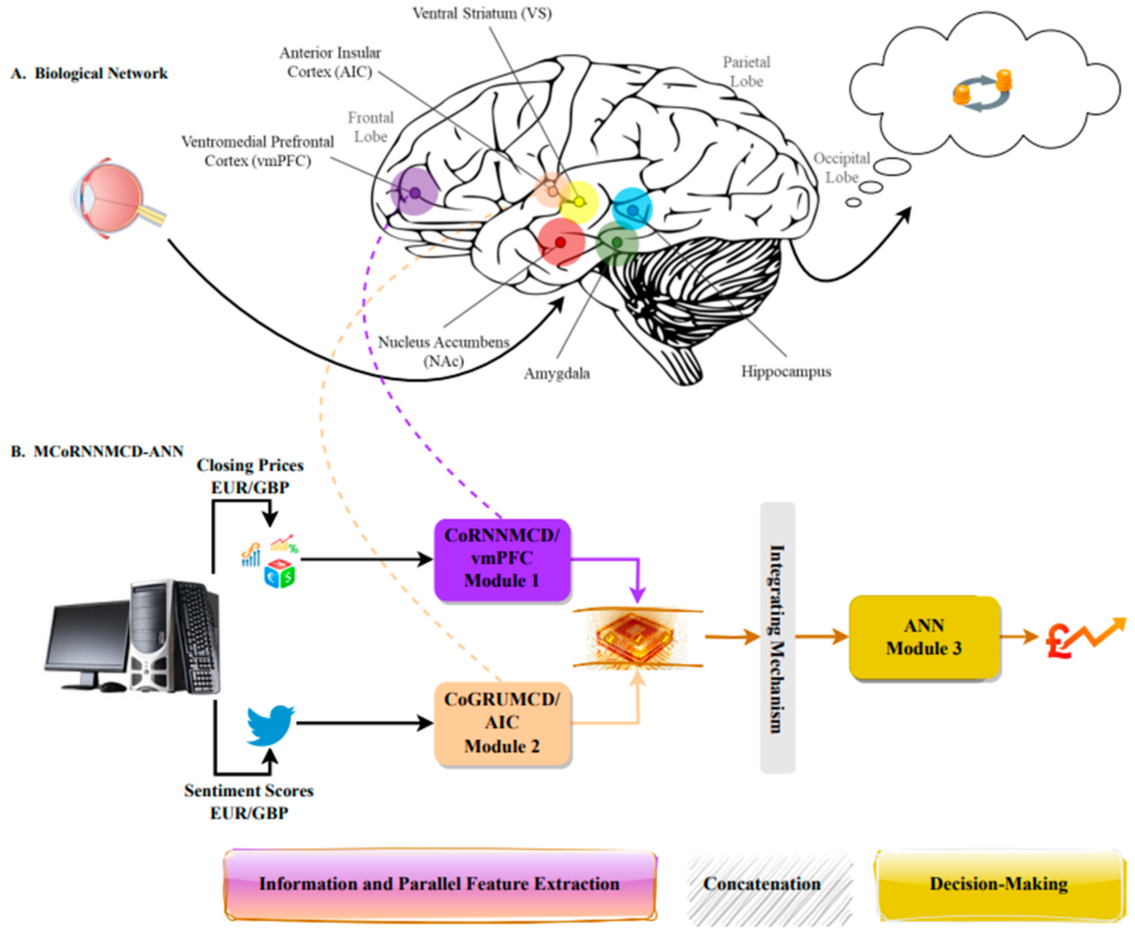
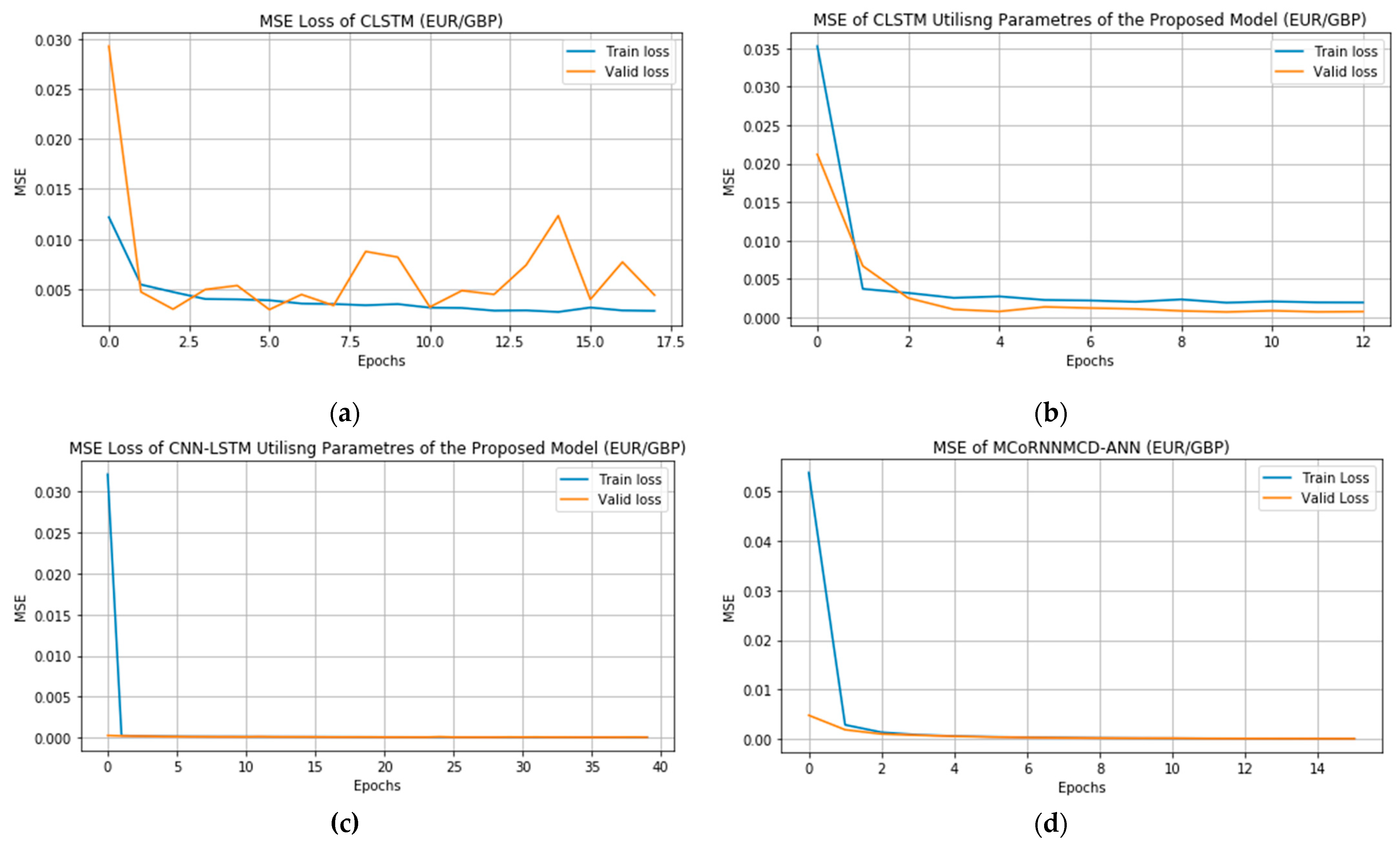
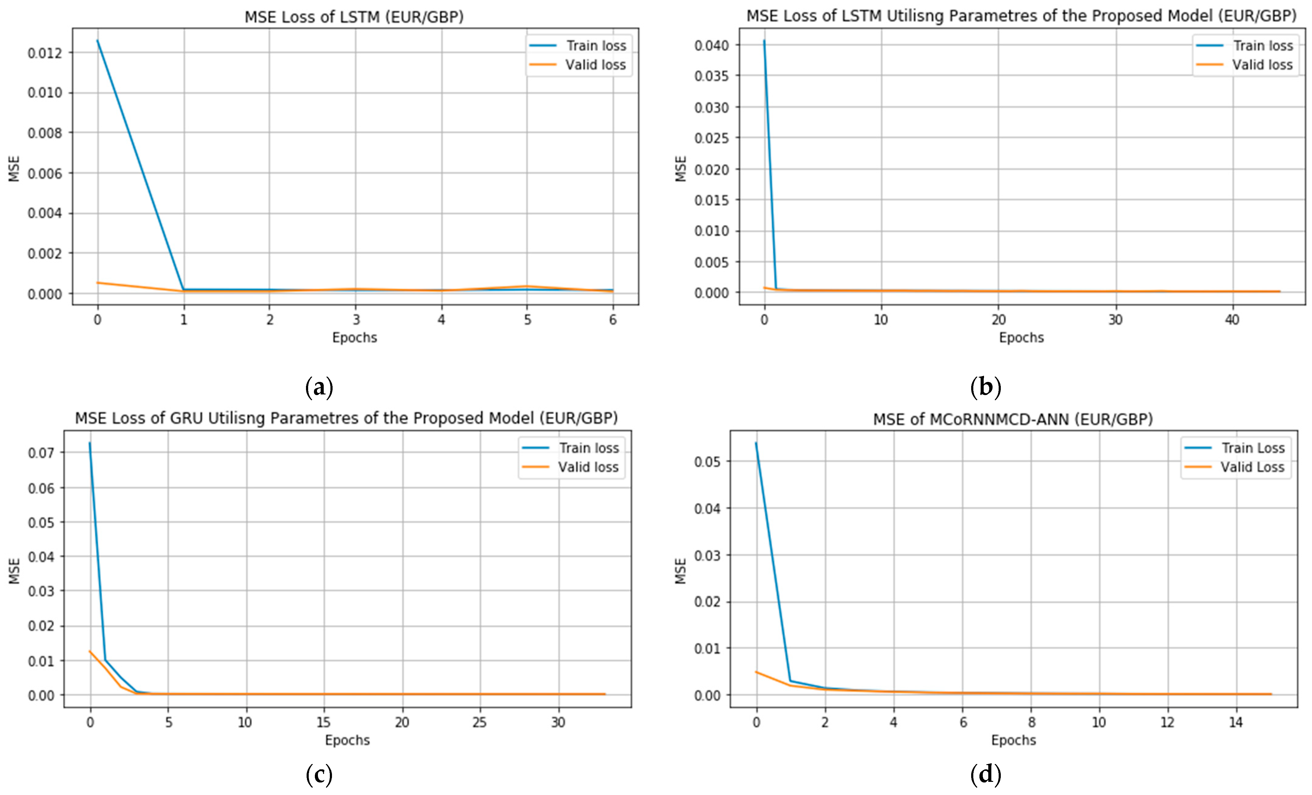
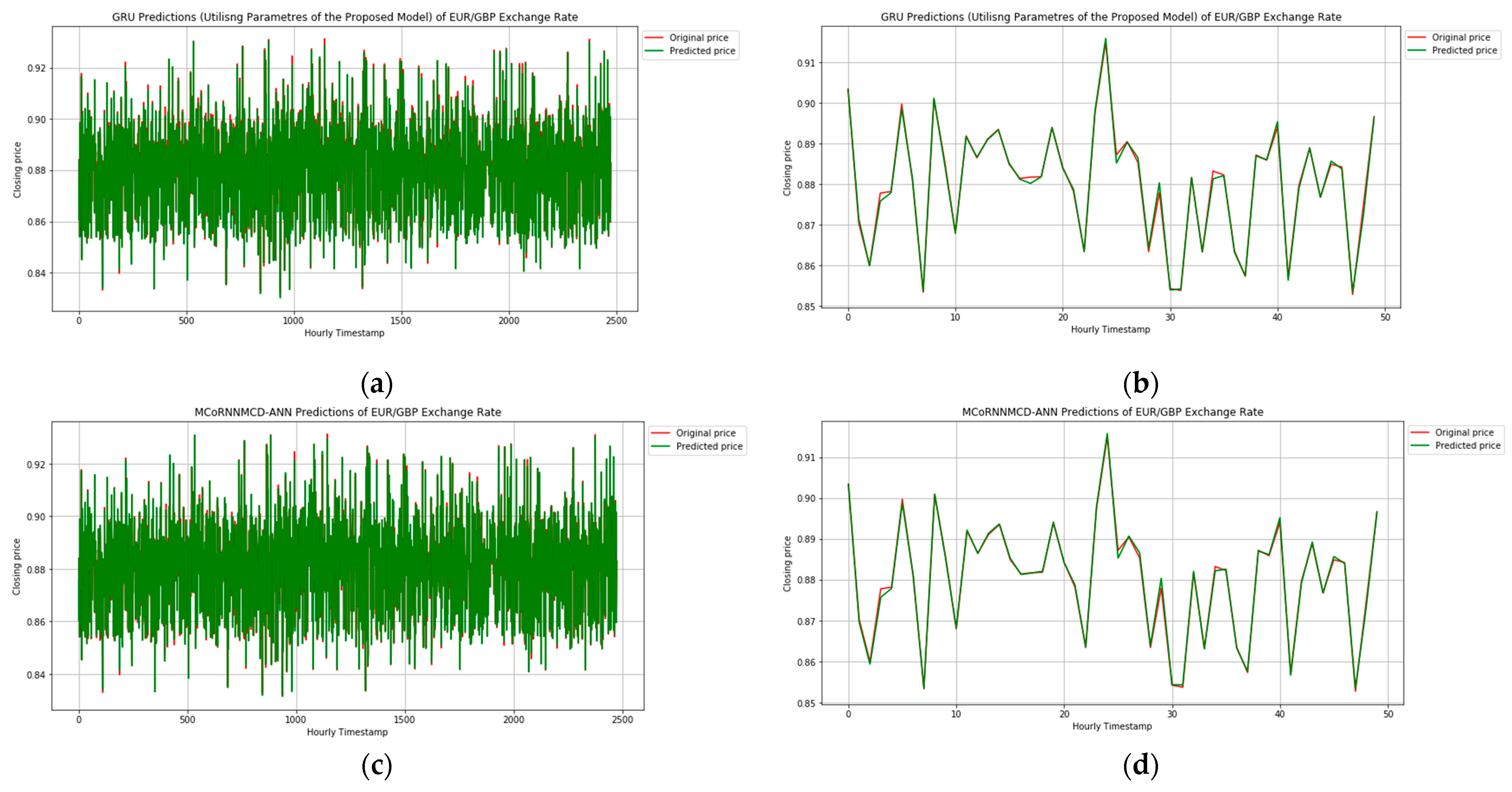
Table 1.
Baseline models performance metrics in closing prices (CP) of EUR/GBP.
| Model | Variables | Metrics | Train | Valid | Test | R2 | Time Duration |
|---|---|---|---|---|---|---|---|
| CoRNNMCD | CP | MSE | 6.7184 × 10⁻⁵ | 6.2938 × 10⁻⁵ | 5.8785 × 10⁻⁵ | 0.99 | 2:30 |
| MAE | 0.00549 | 0.00538 | 0.00529 | ||||
| MSLE | 3.1801 × 10⁻⁵ | 2.79863 × 10⁻⁵ | 2.6419 × 10⁻⁵ | ||||
| CoRNN | CP | MSE | 6.8642 × 10⁻⁵ | 6.3699 × 10⁻⁵ | 5.9447 × 10⁻⁵ | 0.99 | 1:27 |
| MAE | 0.00551 | 0.00541 | 0.00532 | ||||
| MSLE | 3.2413 × 10⁻⁵ | 2.8352 × 10⁻⁵ | 2.6773 × 10⁻⁵ | ||||
| CoGRUMCD | CP | MSE | 6.9541 × 10⁻⁵ | 6.4196 × 10⁻⁵ | 5.9700 × 10⁻⁵ | 0.99 | 7:38 |
| MAE | 0.00551 | 0.00542 | 0.00532 | ||||
| MSLE | 3.3150 × 10⁻⁵ | 2.8718 × 10⁻⁵ | 2.7013 × 10⁻⁵ | ||||
| CoGRU | CP | MSE | 6.9597 × 10⁻⁵ | 6.4106 × 10⁻⁵ | 5.9565 × 10⁻⁵ | 0.99 | 3:59 |
| MAE | 0.00552 | 0.00541 | 0.00532 | ||||
| MSLE | 3.3222 × 10⁻⁵ | 2.8713 × 10⁻⁵ | 2.6914 × 10⁻⁵ | ||||
| 1D-CNN | CP | MSE | 0.00012 | 0.00011 | 0.00011 | 0.99 | 0:36 |
| MAE | 0.00763 | 0.00757 | 0.00747 | ||||
| MSLE | 5.3941 × 10⁻⁵ | 4.800 × 10⁻⁵ | 4.6293 × 10⁻⁵ |
Table 2.
Baseline models performance metrics in sentiment scores of EUR/GBP.
| Model | Variables | Metrics | Train | Valid | Test | R2 | Time Duration |
|---|---|---|---|---|---|---|---|
| CoRNNMCD | Sentiment | MSE | 0.00079 | 0.00076 | 0.00067 | 0.62 | 2:21 |
| MAE | 0.01535 | 0.01512 | 0.01456 | ||||
| MSLE | 0.00031 | 0.00027 | 0.00026 | ||||
| CoRNN | Sentiment | MSE | 0.00077 | 0.00076 | 0.00066 | 0.63 | 1:24 |
| MAE | 0.01504 | 0.01489 | 0.01428 | ||||
| MSLE | 0.00029 | 0.00027 | 0.00025 | ||||
| CoGRUMCD | Sentiment | MSE | 0.00076 | 0.00074 | 0.00065 | 0.64 | 6:09 |
| MAE | 0.01465 | 0.01439 | 0.01394 | ||||
| MSLE | 0.00029 | 0.00026 | 0.00024 | ||||
| CoGRU | Sentiment | MSE | 0.00077 | 0.00075 | 0.00066 | 0.63 | 3:47 |
| MAE | 0.01497 | 0.01479 | 0.01418 | ||||
| MSLE | 0.00030 | 0.00027 | 0.00025 | ||||
| 1D–CNN | Sentiment | MSE | 0.00085 | 0.00083 | 0.00073 | 0.61 | 0:36 |
| MAE | 0.01661 | 0.01644 | 0.01591 | ||||
| MSLE | 0.00034 | 0.00031 | 0.00028 |
Table 3.
Baseline models performance metrics in closing prices in CRNN and sentiment scores in CGRU of EUR/GBP.
Table 3.
Baseline models performance metrics in closing prices in CRNN and sentiment scores in CGRU of EUR/GBP.
| Model | Variables | Metrics | Train | Valid | Test | R2 | Time Duration |
|---|---|---|---|---|---|---|---|
| CRNN | CP | MSE | 6.8795 × 10⁻⁵ | 6.4113 × 10⁻⁵ | 5.9921 × 10⁻⁵ | 0.99 | 1:42 |
| MAE | 0.00530 | 0.00544 | 0.00535 | ||||
| MSLE | 3.2451 × 10⁻⁵ | 2.8487 × 10⁻⁵ | 2.6988 × 10⁻⁵ | ||||
| CGRU | Sentiment | MSE | 0.00079 | 0.00076 | 0.00068 | 0.63 | 3:10 |
| MAE | 0.01577 | 0.01545 | 0.01519 | ||||
| MSLE | 0.00030 | 0.00027 | 0.00026 |
Table 4.
Hybrid models’ performance metrics receive closing prices and sentiment scores of EUR/GBP.
| Model | Metrics | Train | Valid | Test | R2 | Time Duration |
|---|---|---|---|---|---|---|
| BiCuDNNLSTM [64] | MSE | 0.00013 | 0.00015 | 0.00015 | 0.99 | 1:19 |
| MAE | 0.00848 | 0.00874 | 0.00866 | |||
| MSLE | 6.4001 × 10⁻⁵ | 6.6003 × 10⁻⁵ | 6.9725 × 10⁻⁵ | |||
| CNN–LSTM [62] | MSE | 6.4471 × 10⁻⁵ | 5.9427 × 10⁻⁵ | 7.005 × 10⁻⁵ | 0.99 | 1:41 |
| MAE | 0.00538 | 0.00536 | 0.00552 | |||
| MSLE | 3.0273 × 10⁻⁵ | 2.6574 × 10⁻⁵ | 3.2089 × 10⁻⁵ | |||
| LSTM–GRU [60] | MSE | 0.00017 | 0.00014 | 0.00014 | 0.99 | 3:03 |
| MAE | 0.00935 | 0.00901 | 0.00887 | |||
| MSLE | 7.8049 × 10⁻⁵ | 6.3934 × 10⁻⁵ | 6.4782 × 10⁻⁵ | |||
| CLSTM [63] | MSE | 0.00501 | 0.00514 | 0.00507 | 0.79 | 2:18 |
| MAE | 0.05722 | 0.05764 | 0.05743 | |||
| MSLE | 0.00229 | 0.00231 | 0.00234 |
Table 5.
Single models’ performance metrics receive closing prices and sentiment scores of EUR/GBP.
| Model | Metrics | Train | Valid | Test | R2 | Time Duration |
|---|---|---|---|---|---|---|
| 2D–CNN [65] | MSE | 0.00012 | 0.00011 | 0.00012 | 0.99 | 0:51 |
| MAE | 0.00760 | 0.00746 | 0.00765 | |||
| MSLE | 5.3407 × 10⁻⁵ | 4.8839 × 10⁻⁵ | 5.9233 × 10⁻⁵ | |||
| GRU [65] | MSE | 8.7491 × 10⁻⁵ | 7.8116 × 10⁻⁵ | 9.1750 × 10⁻⁵ | 0.99 | 0:47 |
| MAE | 0.00628 | 0.00595 | 0.00614 | |||
| MSLE | 4.0481 × 10⁻⁵ | 3.5261 × 10⁻⁵ | 4.5704 × 10⁻⁵ | |||
| LSTM [65] | MSE | 0.00732 | 0.00723 | 0.00736 | 0.77 | 0:10 |
| MAE | 0.04911 | 0.04911 | 0.04922 | |||
| MSLE | 0.00334 | 0.00327 | 0.00338 |
Table 6.
Top parameters extracted from grid search in closing prices (CP) and sentiment (Sent) scores of EUR/GBP.
Table 6.
Top parameters extracted from grid search in closing prices (CP) and sentiment (Sent) scores of EUR/GBP.
| Model | Lookback | Filters per Convolutional Layer | Nodes per Hidden-Layer | MCD Rate | Batch Size | MSE |
|---|---|---|---|---|---|---|
| CoRNNMCD (CP) | 60 | 128 | 50 | 0.1 | 20 | 0.0010 |
| CoRNNMCD (CP) | 60 | 30 | 30 | 0.1 | 20 | 0.0012 |
| CoGRUMCD (Sent) | 60 | 128 | 50 | 0.1 | 20 | 0.2967 |
| CoGRUMCD (Sent) | 20 | 64 | 30 | 0.1 | 20 | 0.3110 |
Table 7.
MCoRNNMCD–ANN performance metrics in closing prices and sentiment scores of EUR/GBP.
| Model | Metrics | Train | Valid | Test | R2 | Time Duration |
|---|---|---|---|---|---|---|
| MCoRNNMCD–ANN | MSE | 6.5486 × 10⁻⁵ | 6.1332 × 10⁻⁵ | 5.7488 × 10⁻⁵ | 0.99 | 2:35 |
| MAE | 0.00534 | 0.00526 | 0.00518 | |||
| MSLE | 3.1117 × 10⁻⁵ | 2.7342 × 10⁻⁵ | 2.6051 × 10⁻⁵ |
Table 8.
MCoRNNMCD–ANN performance metrics against adjusted (adj.) hybrid benchmarks.
| Model | Metrics | Train | Valid | Test | R2 | Time Duration |
|---|---|---|---|---|---|---|
| BiCuDNNLSTM adj. | MSE | 0.00011 | 0.00010 | 0.00010 | 0.99 | 2:54 |
| MAE | 0.00761 | 0.00754 | 0.00746 | |||
| MSLE | 5.1970 × 10⁻⁵ | 4.7161 × 10⁻⁵ | 4.6294 × 10⁻⁵ | |||
| CNN–LSTM adj. | MSE | 7.2831 × 10⁻⁵ | 6.7592 × 10⁻⁵ | 6.2947 × 10⁻⁵ | 0.99 | 7:13 |
| MAE | 0.00572 | 0.00563 | 0.00551 | |||
| MSLE | 3.4659 × 10⁻⁵ | 3.0217 × 10⁻⁵ | 2.8432 × 10⁻⁵ | |||
| LSTM–GRU adj. | MSE | 0.00011 | 0.00010 | 0.00010 | 0.99 | 20:43 |
| MAE | 0.00739 | 0.00721 | 0.00721 | |||
| MSLE | 5.4301 × 10⁻⁵ | 4.6677 × 10⁻⁵ | 4.6560 × 10⁻⁵ | |||
| CLSTM adj. | MSE | 0.00145 | 0.00151 | 0.00134 | 0.93 | 8:21 |
| MAE | 0.02352 | 0.02381 | 0.02353 | |||
| MSLE | 0.00061 | 0.00063 | 0.00059 | |||
| MCoRNNMCD–ANN | MSE | 6.5486 × 10⁻⁵ | 6.1332 × 10⁻⁵ | 5.7488 × 10⁻⁵ | 0.99 | 2:35 |
| MAE | 0.00534 | 0.00526 | 0.00518 | |||
| MSLE | 3.1117 × 10⁻⁵ | 2.7342 × 10⁻⁵ | 2.6051 × 10⁻⁵ |
Table 9.
MCoRNNMCD–ANN performance metrics against adjusted (adj.) single benchmarks.
| Model | Metrics | Train | Valid | Test | R2 | Time Duration |
|---|---|---|---|---|---|---|
| 2D–CNN adj. | MSE | 0.00017 | 0.00016 | 0.00017 | 0.99 | 0:39 |
| MAE | 0.00901 | 0.00897 | 0.00912 | |||
| MSLE | 8.3038 × 10⁻⁵ | 7.3716 × 10⁻⁵ | 7.6177 × 10⁻⁵ | |||
| GRU adj. | MSE | 7.3054 × 10⁻⁵ | 6.6247 × 10⁻⁵ | 6.2578 × 10⁻⁵ | 0.99 | 4:54 |
| MAE | 0.00558 | 0.00544 | 0.00536 | |||
| MSLE | 3.4814 × 10⁻⁵ | 2.9724 × 10⁻⁵ | 2.8312 × 10⁻⁵ | |||
| LSTM adj. | MSE | 8.7955 × 10⁻⁵ | 8.0258 × 10⁻⁵ | 7.6894 × 10⁻⁵ | 0.99 | 8:43 |
| MAE | 0.00635 | 0.00621 | 0.00612 | |||
| MSLE | 4.1941 × 10⁻⁵ | 3.6171 × 10⁻⁵ | 3.4807 × 10⁻⁵ | |||
| MCoRNNMCD–ANN | MSE | 6.5486 × 10⁻⁵ | 6.1332 × 10⁻⁵ | 5.7488 × 10⁻⁵ | 0.99 | 2:35 |
| MAE | 0.00534 | 0.00526 | 0.00518 | |||
| MSLE | 3.1117 × 10⁻⁵ | 2.7342 × 10⁻⁵ | 2.6051 × 10⁻⁵ |
Disclaimer/Publisher’s Note: The statements, opinions and data contained in all publications are solely those of the individual author(s) and contributor(s) and not of MDPI and/or the editor(s). MDPI and/or the editor(s) disclaim responsibility for any injury to people or property resulting from any ideas, methods, instructions or products referred to in the content. |
© 2023 by the authors. Licensee MDPI, Basel, Switzerland. This article is an open access article distributed under the terms and conditions of the Creative Commons Attribution (CC BY) license (https://creativecommons.org/licenses/by/4.0/).
Share and Cite
MDPI and ACS Style
Bormpotsis, C.; Sedky, M.; Patel, A. Predicting Forex Currency Fluctuations Using a Novel Bio-Inspired Modular Neural Network. Big Data Cogn. Comput. 2023, 7, 152. https://doi.org/10.3390/bdcc7030152
AMA Style
Bormpotsis C, Sedky M, Patel A. Predicting Forex Currency Fluctuations Using a Novel Bio-Inspired Modular Neural Network. Big Data and Cognitive Computing. 2023; 7(3):152. https://doi.org/10.3390/bdcc7030152
Chicago/Turabian StyleBormpotsis, Christos, Mohamed Sedky, and Asma Patel. 2023. "Predicting Forex Currency Fluctuations Using a Novel Bio-Inspired Modular Neural Network" Big Data and Cognitive Computing 7, no. 3: 152. https://doi.org/10.3390/bdcc7030152