Evaluating the Robustness of Deep Learning Models against Adversarial Attacks: An Analysis with FGSM, PGD and CW

Abstract

This study evaluated the generation of adversarial examples and the subsequent robustness of an image classification model. The attacks were performed using the Fast Gradient Sign method, the Projected Gradient Descent method, and the Carlini and Wagner attack to perturb the original images and analyze their impact on the model’s classification accuracy. Additionally, image manipulation techniques were investigated as defensive measures against adversarial attacks. The results highlighted the model’s vulnerability to conflicting examples: the Fast Gradient Signed Method effectively altered the original classifications, while the Carlini and Wagner method proved less effective. Promising approaches such as noise reduction, image compression, and Gaussian blurring were presented as effective countermeasures. These findings underscore the importance of addressing the vulnerability of machine learning models and the need to develop robust defenses against adversarial examples. This article emphasizes the urgency of addressing the threat posed by harmful standards in machine learning models, highlighting the relevance of implementing effective countermeasures and image manipulation techniques to mitigate the effects of adversarial attacks. These efforts are crucial to safeguarding model integrity and trust in an environment marked by constantly evolving hostile threats. An average 25% decrease in accuracy was observed for the VGG16 model when exposed to the Fast Gradient Signed Method and Projected Gradient Descent attacks, and an even more significant 35% decrease with the Carlini and Wagner method.

1. Introduction

The increasing adoption of neural networks in various fields has significantly advanced processing and pattern recognition in complex data, such as images, text, and speech. However, these networks have also been shown to be susceptible to malicious attacks by generating adversarial examples [1]. Hostile instances are carefully designed to trick neural network models into misclassifying input data. Generating negative illustrations have become a topic of great interest in the machine learning and cybersecurity research community. Understanding how these adversarial instances are created and developing effective countermeasures is essential to improving the security and reliability of neural network-based applications [2].

This article explores the process of generating adversarial examples and the countermeasures used to mitigate these attacks. The theoretical foundations behind the development of negative models are examined, including concepts such as the loss function and gradient optimization [3]. Additionally, three popular algorithms used to generate adversarial examples are discussed: the fast gradient sign method (FGSM), the projected gradient downward (PGD), and the Carlini–Wagner (CW) method [4,5,6,7]. The FGSM algorithm is one of the simplest and most widely used methods for generating adversarial examples. This paper discusses using the gradient of the loss function to perturb the input data imperceptibly but enough to induce errors in model classification [8]. We will show examples of original and perturbed images using FGSM and their effectiveness in different scenarios will be discussed.

In the same way, the PGD algorithm is applied in this study, which is an extension of the FGSM that performs multiple iterations of gradual perturbation to increase the effectiveness of the adversary attack [9]. We analyze how the PGD uses a search strategy in the input space to find adversarial examples that are more difficult to detect and correct. In addition, the CW method is explored, which takes a more complex optimization approach to generate negative models. We analyze how the CW minimizes a specific cost function to find the optimal perturbation that induces a misclassification with high confidence [10].

While generating adversarial examples is a significant concern, addressing countermeasures to protect neural network models against these attacks is also critical. Therefore, this paper identifies and applies the countermeasures used to defend against adversary examples [11]. Thus, approaches such as denoising filtering, image compression, and Gaussian blurring are discussed, which are used to pre-process images and reduce the impact of adversarial disturbances. With this, we discuss how these methods can improve the robustness of neural network models against hostile example generation attacks.

This paper presents experimental and comparative results to evaluate the algorithm’s effectiveness in generating adversary examples and implementing countermeasures. Popular data sets such as MNIST and CIFAR-10 and widely used neural network models such as Visual Geometry Group 16 (VGG16) and ResNet are used for testing and analysis.

When analyzing the results obtained, the objective of providing an exhaustive version of generating adversarial examples and countermeasures in neural networks is met. By understanding the theoretical foundations, negative example generation algorithms, and available countermeasures, machine learning researchers and practitioners can strengthen their models’ security and safeguard neural network-based applications [12]. Furthermore, this article delves into each critical aspect, presenting concrete examples and discussing the security implications and limitations of the different techniques.

In this article, we first present, in Section 1, the introduction to the problem of adversarial examples and their importance in the security of machine learning models. In Section 2, we review similar works in this field and highlight the relevance and innovation of our approach. In Section 3, subsequently, we describe the methods used to generate adversarial examples, including FGSM, PGD, and CW, along with their respective implementations and parameter settings. Section 4 focuses on our experiments and results, where we evaluate the effectiveness of these methods in different scenarios. Additionally, we discuss the importance of execution times and the balance between accuracy and efficiency. Then, in Section 5, we present and discuss the implications of our research. In Section 6, we offer our conclusions and suggest future directions for research in this field.

2. Review of Related Works

There is growing concern about the security and robustness of neural network models against adversarial examples. Numerous researchers have approached this challenge from different angles, proposing techniques and algorithms to generate negative examples and develop effective countermeasures. In our review of similar works, an analysis of those that have stood out in this field is presented, and we evaluate it according to the relevance and innovation of our proposal. One of the pioneering works in this field is Liang et al. [13]. In this study, the FGSM algorithm was introduced, which proved effective in fooling machine learning models. Although this work laid the foundations for the generation of adversarial examples, our proposal goes further by addressing not only the age of negative examples but also the implementation of countermeasures to improve the robustness of the models.

In the work of Madry et al. [14], the PGD method was proposed as a more effective technique to generate adversarial examples and improve the resistance of the models. Our proposal aligns with this research using the FGSM algorithm and the PGD method to generate malicious samples. Still, we also explore other techniques, such as generating non-differentiable negative examples and manipulating specific features. Another relevant study is Ren et al. [15], which comprehensively reviews adversarial example generation methods and countermeasures in neural networks. Unlike this work, our proposal focuses on reviewing and analyzing existing approaches and seeks to provide new perspectives and innovative solutions. Our policy is based on combining different adversarial example generation algorithms and implementing specific countermeasures to improve the robustness of the models.

The work of Buckman et al. [16] is interesting as it proposes using thermometer coding as a countermeasure against adversarial examples. While this technique has proven effective, our proposal explores multiple defense approaches, such as adversary training, adversary instance detection, and robustness enhancement through feature manipulation. Furthermore, Sharif et al. [17] investigated using nearest neighbor (K-NN) algorithms as a defense strategy against adversarial examples. Although this approach has shown promising results, our proposal differentiates itself by combining multiple adversarial example generation techniques and countermeasures, allowing for a more robust and adaptable defense against attacks.

Although several works are related to generating adversarial examples and countermeasures in neural networks, our proposal stands out for its comprehensive approach and combination of different techniques and algorithms. This addresses not only the generation of adversarial examples but also the implementation of specific countermeasures to improve the robustness of the models. In addition, the approach of this work innovates by exploring new techniques, such as the generation of non-differentiable adversarial examples and the manipulation of specific features. The experiments and results demonstrate the relevance and effectiveness of our proposal in protecting machine learning models against adversary attacks.

Table 1. Results of adversarial example generation methods.

Author	Proposed Method	Main Contributions	Key Results
Wang et al. [18]	FGSM	Introduction of the FGSM method in the generation of adversarial examples.	Effective results in manipulating ML models.
Cheng et al. [19]	PGD	Development of the PGD method as an effective technique to generate adversarial examples.	Greater robustness against adversary attacks.
Carrillo-Perez et al. [20]	Comprehensive Review	Comprehensive analysis of methods and countermeasures in neural networks.	Identification of gaps and new perspectives in the field.
Vardhan et al. [21]	Thermometer Coding	Proposal for thermometer coding as a countermeasure.	Improved robustness against adversarial examples.
Gupta et al. [22]	K-NN	Investigation of the application of K-NN algorithms as a defense against adversarial examples.	Promising results in attack detection and prevention.

summarizes the most notable related works in this area, highlighting their proposed plans, the main contributions they made, and the key results obtained. Notably, one of the first significant advances in this field was achieved by introducing the FGSM method by Wang et al. [18]. This was shown to be effective in manipulating machine learning models by Cheng et al. [19]. On the other hand, they proposed the PGD method as a more effective technique to generate adversarial examples and improve the robustness of the models. Additionally, Carrillo-Perez et al. [20] comprehensively reviewed methods and countermeasures in neural networks, identifying gaps and new perspectives in the field. Other approaches, such as thermometer coding proposed by Vardhan et al. [21] and applying K-NN algorithms as defense, as investigated by Gupta et al. [22], have shown promising results in detecting and preventing adversarial attacks.

3. Materials and Methods

The method used in this work to address the problem of generating adversarial examples and developing effective countermeasures in neural networks is based on the analysis of similar results in this field and several concepts that are the basis for implementing adversarial standards and their countermeasures.

Furthermore, a comprehensive and novel approach is presented to address the security of neural networks, such as defending against attacks from adversarial examples. This contribution is distinguished by its comprehensive approach, which combines the generation of adversarial examples using multiple algorithms, including FGSM, PGD, and CW, with helpful defense strategies. Through experimentation, we reveal valuable insights into the effectiveness of various defense techniques and their impact on the robustness of machine learning models.

3.1. Concepts Used

The concepts used in this work are essential to understanding the context and the proposed methodology. These concepts are used to explore the generation of adversarial examples and countermeasures in neural networks. As well as implementing algorithms such as the FGSM, the PGD, and the CW to generate negative examples, specific countermeasures are developed to strengthen the robustness of the models [23]. In addition, regularization techniques and other approaches to improve detectability and defense against adversarial examples are considered. Combining these concepts makes it possible to obtain promising results, and we contribute to advancing research in this field.

Adversarial examples are data instances carefully crafted to fool machine learning models. These examples are generated by imperceptible modifications to the original input data to cause the model to make wrong or undesirable predictions [24]. Adversary samples can be used to assess the robustness of models or as malicious tools to bypass security systems based on machine learning.

Neural networks are computational models inspired by the functioning of the human brain. These networks comprise layers of interconnected nodes, called neurons, that process and transmit information [25]. Neural networks are widely used in machine learning to perform pattern recognition, classification, and prediction generation tasks.

Supervised learning is a machine learning model training technique in which input examples are provided along with expected results. The model learns by comparing its predictions with the desired results and adjusting its internal parameters to minimize the difference. This approach is commonly used in image classification, where models are trained to assign correct labels to new images.

The FGSM algorithm is a popular technique for rapidly generating adversarial examples. It is based on calculating the gradient of the model’s loss function concerning the input data. Then, the input data is slightly modified in the gradient direction to maximize the loss and fool the model. The FGSM algorithm is simple and efficient, but it can generate adversarial instances easily detectable by more sophisticated countermeasures.

The PGD algorithm is an extension of the FGSM algorithm that seeks to generate more robust and difficult-to-detect adversarial examples. Instead of performing a single perturbation in the gradient direction, the PGD algorithm performs multiple iterations, limiting the magnitude of the displacement (or perturbation) in the gradient direction in each iteration [26]. This allows you to explore a broader search space and generate more effective adversarial examples.

Countermeasures are techniques and strategies used to improve the robustness of machine learning models against adversarial examples. These techniques can include the implementation of adversarial example detection algorithms, incorporating defense mechanisms in the model training process, and introducing random disturbances in the input data, among other approaches [27].

Regularization is a technique used to prevent the overfitting of machine learning models. It consists of adding a term to the loss function of the model that penalizes the most complex models or those that have parameters with high values. Regularization helps control the model’s capability and improves its generalizability, which can help make it more resilient to adversarial examples.

3.2. Metrics Used

For comprehensive evaluation, the following metrics are used to measure model performance:

• Accuracy: This metric measures the fraction of images correctly classified by the model. It is calculated as:

$$Accuracy=\frac{Number of correct predictions}{Total number of predictions}$$

(1)

• F1 Score: The F1 score is a metric that combines precision and completeness into a single measure. It is beneficial when dealing with unbalanced classes. It is calculated as:

$$F1 Score=\frac{2\ast Precision\ast Recall}{Precision+Recall}$$

(2)

• Confusion Matrix: The confusion matrix shows how many images were classified into each class and how many of those classifications were correct or incorrect. This provides detailed information about the performance of the model in each category.
• Precision: Also known as positive predictive value, it measures the precision of the model’s positive predictions. It is calculated as:

$$Precision=\frac{True positives}{True positives+False positives}$$

(3)

• Recall: Completeness, also known as sensitivity or true positive rate, measures the model’s ability to capture all positive examples. It is calculated as:

$$Recall=\frac{True positives}{True positives+False negatives}$$

(4)

• Specificity: Specificity measures the model’s ability to capture all negative examples. It is calculated as:

$$Specificity=\frac{True negatives}{True negatives+False positives}$$

(5)

3.3. Method

The method used in this paper is based on a combination of adversarial example generation techniques, model robustness analysis, and countermeasure strategies. The main objective is to explore and evaluate the effectiveness of different adversarial example generation algorithms and develop countermeasures that improve the resistance of models against these misleading examples.

Figure 1 shows the main stages of the method, which start with loading a pre-trained model and preprocessing the input image. Adversarial sample generation algorithms create misleading samples fed into the model. The FGSM algorithm is implemented, a widely used technique to generate adversarial examples quickly and efficiently [28]. This algorithm is based on computing the gradient of the model’s loss function concerning the input data and then perturbs in the direction of the gradient to maximize the loss and fool the model. In addition to the FGSM algorithm, we also implement the PGD algorithm, which performs multiple iterations of small perturbations on the input data, limiting the norm of perturbations at each iteration. This allows you to explore a broader search space and generate more effective adversarial examples that are difficult to detect and counter.

The next stage is to evaluate the robustness of the models in the face of the adversary examples generated, for which metrics such as the success rate of adversary attacks are used, which measures the proportion of adversary examples that manage to deceive the model, and the rate of detection of implemented countermeasures, which measures the ability of countermeasures to identify and neutralize adversary instances [29].

Countermeasure strategies are then implemented to strengthen the resilience of the models against adversarial examples. These strategies include incorporating regularization techniques in the model training process, introducing random disturbances in the input data, and implementing adversarial example detection algorithms. Countermeasures include regularization techniques during training, introducing random perturbations into the input data, and implementing adversarial example detection algorithms. These measures seek to improve the resistance of the model against the adversarial examples generated. During the development of this work, exhaustive experiments and evaluations are carried out to analyze the impact of the adversarial example generation algorithms and the effectiveness of the implemented countermeasures.

The approach is based on combining existing techniques and exploring new strategies to improve the robustness of the models and mitigate the effects of adversarial examples. In the next stage, the experimental process is detailed, including the data sets, the configuration of the models, and the evaluation procedures [30]. In this case, the effectiveness of these adversary examples is evaluated, and we proceed to implement countermeasures to strengthen the robustness of the model. Finally, we assess the resistance of the model against the adversarial examples and conclude the process.

3.4. Design of Adversary Examples

Different algorithms, such as FGSM, PGD, and CW, have been used to design adversarial examples. The FGSM method is a simple but effective algorithm for generating adversarial examples. This method uses the gradient of the loss function relative to the input image to compute a perturbation that maximizes the loss function. The perturbation is added to the original image to generate an adversarial instance [31]. The input image is loaded and converted to a floating-point tensor for the implementation. The VGG16 pre-trained model is used to obtain the class predictions for the input image. The gradient of the loss function relative to the input image is calculated. The gradient is used to calculate the perturbation using the sign function. Finally, the perturbation is added to the original image to obtain the adversary example.

The FGSM generates adversarial examples by applying small perturbations in the gradient direction of the model loss function. The loss function L is typically calculated as the difference between the model prediction and the actual label. For an example of input x and its label y, the loss function L(x,y) is calculated, and then the gradient of this loss function concerning the input x is obtained, denoted as ${\nabla }_{x}L(x,y)$. The perturbation is calculated using the gradient sign function and multiplied by a factor ∈, representing the perturbation’s magnitude. The adversary image is then obtained as follows:

$$x^{\prime }=x+\in ·sign\left({\nabla }_{x}L\right(x,y\left)\right)$$

(6)

The PGD method is a variant of the FGSM that seeks to generate more robust and difficult-to-detect adversary examples. PGD performs multiple iterations to update the perturbed image and find the optimal perturbation [32]. The PGD algorithm follows the following steps:

• Specific hyperparameters are defined for the method, such as the perturbation size (epsilon), the learning rate (alpha), and the number of iterations.
• The perturbed image is initialized as a copy of the original image.
• A loop of iterations is executed to update the perturbed image:
  • The gradient of the loss function concerning the perturbed image is calculated.
  • A fraction of the gradient (determined by alpha) is added to the perturbed image.
  • A projection is applied to keep the disturbance within an allowable range.
• The perturbed image is returned as the generated adversarial example.

PGD is an extension of FGSM that incorporates multiple iterations. A small perturbation is applied in each iteration, and the resulting example is projected within an allowed range to ensure that it does not stray too far from the original. This iterative process can be described as:

• Initialize $x_0^{\prime }=x$.

For each iteration i, update x′ by

$$x_{i+1}^{\prime }=Projection(x_i^{\prime }+\alpha ·sign \left({\nabla }_{x}L\left(x_i^{\prime },y\right)\right),\in )$$

(7)

where α is the learning rate and the Projection function ensures that x′ remains within the allowed range.

The CW algorithm is a sophisticated technique for generating adversarial examples. It uses a more complex loss function and optimization approach to find the optimal perturbation that maximizes the loss function and meets certain constraints [4].

The input image is loaded and converted to a floating-point tensor. Specific hyperparameters are defined for the method, such as the target class, desired confidence, learning rate, and number of iterations. The perturbed image is initialized as a tensor variable. A loop of iterations is performed to optimize the perturbed image. Model predictions for the image are calculated. The CW loss function is computed considering the confidence and constraints.

Next, the gradient of the loss function relative to the perturbed image is calculated. The perturbed image is updated using the gradient and learning rate. A projection is applied to keep the disturbance within the allowed range. Finally, the angry image is returned as a generated adversary instance.

The choice of parameters is essential to understand the effectiveness and applicability of the methods in different scenarios. The critical parameter values used in the experiments to generate adversarial examples and evaluate the robustness of the models are as follows. The learning rate: the learning rate is crucial to our experiments. We used a learning rate of 0.01 for the FGSM algorithm and 0.001 for the PGD method. These values were selected after an adjustment process considering the convergence speed and the models’ stability. Number of iterations: in the case of the PGD method, we determined that 40 iterations are optimal to balance the generation of compelling adversarial examples with execution time. This number of iterations allowed for a proper balance between the effectiveness of the perturbation and the attack.

Epsilon: the epsilon parameter controls the magnitude of the perturbations applied to the input samples. We set epsilon to 0.3 for the FGSM method and 0.1 for the PGD method. These values were chosen after experimenting with different perturbation levels and evaluating their impact on the ability to fool the models. Batch size: we used a batch size of 32 to generate adversarial examples in our experiments. This value was selected considering the processing capacity of our experimental environment and computational efficiency. Machine learning models: we detail the specific architectures of the machine learning models used in our experiments, including the model type (e.g., convolutional neural network) and its complexity. Hardware and Software Environment: we describe the hardware and software used in our experiments, including the type of CPU/GPU, the amount of RAM, and the operating system. This provides essential information about the test environment.

The settings of these parameters are based on previous experiences and experiments to ensure consistent and comparable results. These values can be adjusted based on the specific needs of individual applications, but our choice is intended to provide a solid foundation for our research.

3.5. Implementation of Algorithms with Adversarial Examples and Countermeasures

In addition to the algorithms mentioned above, in this work, a proprietary algorithm is developed to improve the generation of adversarial examples [33]. This algorithm combines aspects of FGSM, PGD, and CW to obtain adversarial examples that are both effective and invisible. Figure 2 shows the general flow of the algorithm:

• The input image is loaded and converted to a floating-point tensor in the first phase.
• The pre-trained model VGG16 is used to obtain the class predictions for the input image.
• Next, the initial disturbance is calculated using the FGSM method.
• In the next phase, an iterative refinement process is applied using the PGD method, updating the disturbed image in each iteration.
• We use the CW method to tune the disturbance further and improve the adversary example’s effectiveness.
• Post-processing techniques such as denoising filters, JPEG compression, and Gaussian blur are then applied to improve the imperceptibility of the adversary pattern.
• Finally, the model’s classification for the generated adversary example is evaluated.

With the implementation of these algorithms and the approach proposed in this work, we seek to explore different methods of generating adversarial examples and demonstrate their effectiveness in deceiving image classification models [34]. For their part, the countermeasures used are techniques to increase the robustness and resistance of machine learning models against adversary attacks. In this work, three countermeasure techniques have been applied, and they are included in the developed algorithm to verify its operation and behavior in the designed environment.

The first countermeasure used is the detection of adversary attacks. An effective countermeasure consists of detecting the presence of an adversary attack. This can be achieved by comparing specific features of the original and disturbed images. For example, the pixel differences between the authentic and restless images can be calculated. If the differences exceed a set threshold, the presence of an adversary attack can be inferred. In the design of the algorithm, the code has been implemented, and an additional function called “detect_adversarial_attack (image, disturbed_image)” is added, which takes the original image and the disturbed image as input and performs pixel difference comparison. If an adversarial attack is detected, corresponding actions can be taken, such as rejecting the classification or performing additional validation processing.

In a real scenario, implementing methods to detect perturbed inputs can be challenging, especially when the original image is unavailable for comparison. In such cases, machine learning models can be trained to identify anomalies or unusual patterns, indicating an image has been altered. This is achieved by training the model with a data set that includes original and perturbed images, allowing the model to learn to differentiate between the two. Additionally, anomaly detection or consistency analysis can improve the model’s ability to identify perturbed inputs without the original images.

Another countermeasure is adversarial training, which involves training the machine learning model using generated examples [35]. This helps the model learn and understand the characteristics of adversary attacks, improving its ability to resist future attacks. In the implementation, “generate_pgd_example” generates adversarial examples for evaluation and use during training. This involves developing adversarial examples using the PGD method with parameter variations, such as epsilon and alpha, and then adding these examples to the training set along with the original images.

The following countermeasure used is adversarial regularization, which involves adding additional terms to the loss function during training to penalize adversarial disturbances. These terms are intended to minimize an attacker’s ability to significantly disrupt input images without affecting correct classification. In its implementation, the loss function used in training the model is modified to include an adversary regularization term [36]. This is achieved by calculating the adversarial loss between the model predictions for the original and disturbed images and then adding this damaging loss to the total loss during training.

3.6. Experimental Procedures and Data Splitting

The experimental methodology covers various crucial aspects to evaluate the proposed models’ performance rigorously. The following points provide a detailed description of each of these aspects:

• Data Division: To ensure a fair and robust evaluation of the model, the data set was divided into three main collections: training, validation, and testing. The division was carried out following a proportion of 70% for training, 15% for validation, and 15% for testing. This split ensures that the model is trained on a large amount of data and evaluated on independent sets.
• Data Augmentation: Data augmentation techniques were applied to diversify the training set further and improve the model’s generalization ability. These techniques included random rotation, rescaling, cropping, and brightness and contrast changes. Each image in the training set was subjected to these transformations to create additional variations of the original images.

3.6.1. Evaluation Metrics

Evaluation of model performance was based on several key metrics, including:

• Precision: The fraction of images correctly classified by the model.
• Key Metrics: In addition to precision, it is essential to evaluate metrics such as F1 score, precision, and completeness. The F1 score is a metric that combines precision and completeness, which is especially useful when classes are unbalanced.
• F1-Score: A metric that combines precision and completeness, handy when classes are unbalanced.
• Confusion Matrix: Examining the confusion matrix is essential to understanding how the model classifies the different classes. This allows you to identify where the model struggles and where it succeeds. It can help discover if the model tends to misclassify certain types or is more accurate with some classes than others. Provides a detailed view of how the model classifies different classes and helps identify potential problem areas.
  • Specificity: Measures the model’s ability to correctly identify negative examples.
  • Sensitivity: Measures the model’s ability to correctly identify positive examples.
• “Out of Sample” Images: To guarantee the objectivity of the evaluation, it is essential to use images that have not been previously used in the training process or the validation of the model. These out-of-sample images better reflect model performance in real-world situations and avoid overestimating model performance.
• Expanding the Evaluation Data Set: Increasing the number of evaluation images improves the reliability of the results. A more extensive evaluation data set reduces the influence of random fluctuations on the metrics and provides a more robust evaluation of the model.
• Image Class Diversity: Exploring model performance on different image classes, such as human faces, artificial objects, or other categories relevant to the application domain, provides a more complete view of the impact of the proposed methods.

3.6.2. Parameter Configuration

During the experiments, several parameters were tuned to optimize the performance of the adversarial example generation algorithms. These parameters included learning rate, number of iterations, and perturbation size. Specific configurations were selected through a fitting process considering model convergence and stability.

To ensure the robustness of the results, five-fold cross-validation was used instead of a single data split. This allowed for a more robust evaluation of the model’s performance by testing it on different subsets of the data. In addition to validation on the primary data set, the models were evaluated on multiple additional data sets to understand their performance in various scenarios better. The experiments were conducted in an environment with an Intel Core i9 processor and an NVIDIA GeForce RTX 3090 graphics card. This provides information about the hardware used and the software environment, including the operating system and available RAM.

Comprehensive evaluation helps to understand better how the proposed methods affect model performance and ensures the validity and robustness of the results. With a more complete assessment, more informed decisions can be made about the effectiveness and appropriateness of the approaches used.

4. Results

The classification of the original and disturbed images with the applied countermeasures is shown to analyze the results. Additionally, decode_predictions are used to obtain readable labels from the model predictions.

Table 2. Results of Adversarial Example Generation Methods.

	Initial Prediction	FGSM Results	PGD Results	CW Results
Class 1	beagle (0.383)	Weimaraner (0.498)	Weimaraner (0.625)	Greater_Swiss_Mountain_dog (0.527)
Class 2	English foxhound (0.352)	Walker_hound (0.142)	Walker_hound (0.097)	beagle (0.138)
Class 3	Entlebucher (0.127)	German_short-haired_pointer (0.114)	German_short-haired_pointer (0.089)	Entlebucher (0.128)

shows the initial and disturbed results. This table shows the initial predictions and the results after applying the adversary examples using the FGSM, PGD, and CW methods. Each column represents an object class, and the values in parentheses correspond to the prediction probabilities.

For the analysis, the pre-trained model VGG16 is used; this makes the class predictions for each input image; one of the examples carried out uses the image of a Beagle, as shown in Figure 3. In the initial prediction, the model classified the image as a “beagle”, with a probability of 38.3%. This indicates that the model had high confidence in the original classification. However, it also assigned significant probabilities to other classes, such as “English_foxhound” (35.2%) and “Entlebucher” (12.7%).

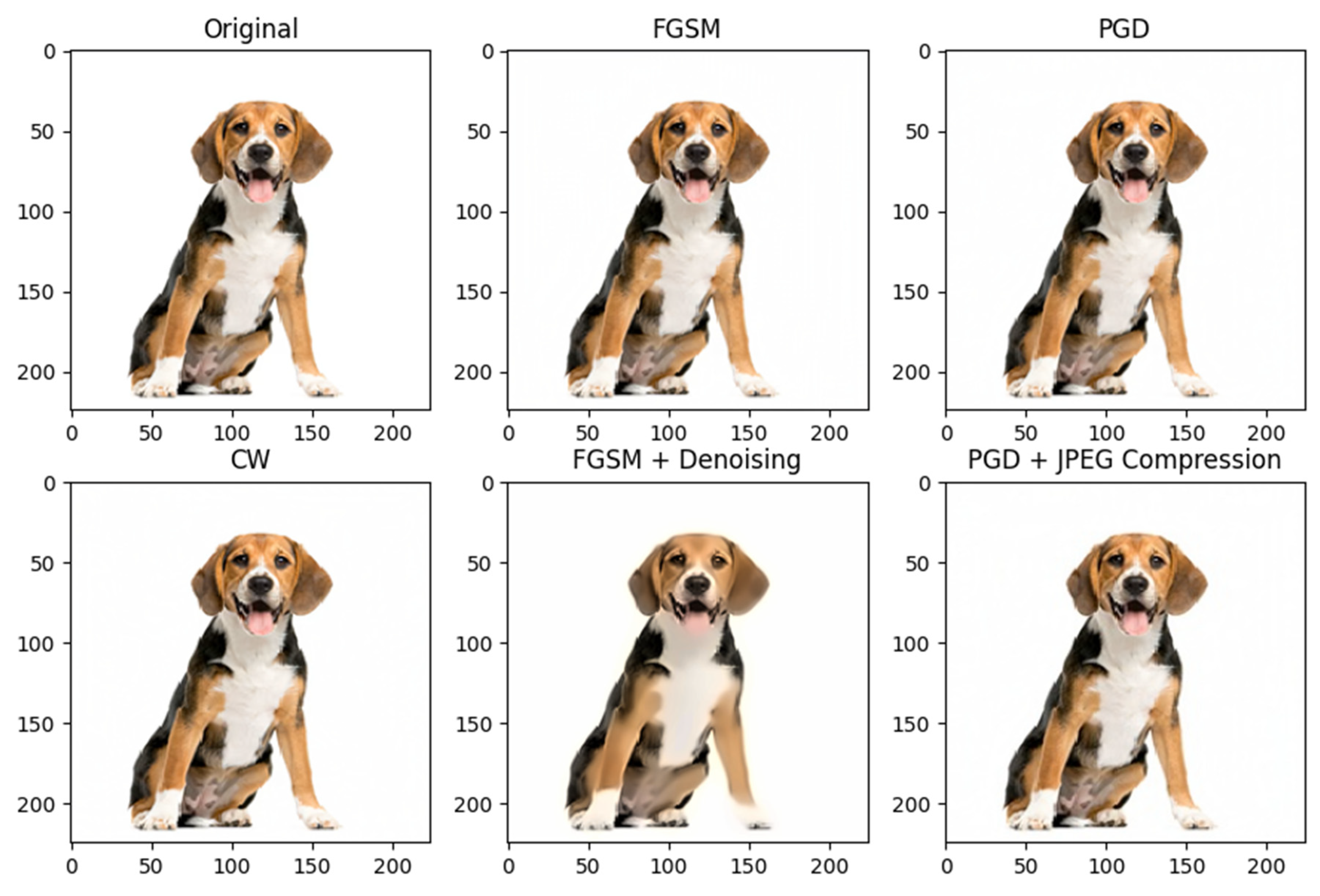
Figure 3 shows the visual results of applying adversarial attacks using FGSM, PGD, and CW techniques to an image of a dog. While the adversarial examples generated by FGSM and PGD maintain a visual appearance close to the original image, the CW attack results in an image with noticeable color distortion and an unrealistic overall appearance. This result underlines the power of the CW attack to generate adversarial examples that not only fool machine learning models but also create extreme visual disturbances that are easily perceptible by humans, questioning its usefulness in practical scenarios where discretion is vital.

When applying the FGSM method, a change in the model predictions is observed. The “beagle” class (original prediction) is replaced by the “Weimaraner” class as the most likely prediction, with a probability of 49.8%. This indicates that the adversarial example generated using FGSM was able to fool the model into misclassifying the image as a “Weimaraner”. The original classes, such as “English_foxhound” and “Entlebucher”, also get significant probabilities, albeit lower than the new prevailing class.

Using the PGD method, a more drastic change in the model predictions is observed. The “Weimaraner” class becomes even more dominant, with a probability of 62.5%. This indicates that the adversarial example generated with PGD managed to fool the model more effectively than FGSM. The original classes, such as “English_foxhound” and “Entlebucher”, get much lower probabilities than the initial predictions.

Using the CW method, another variation in the model predictions is produced. The “Greater_Swiss_Mountain_dog” class becomes the most likely prediction, with a probability of 52.7%. This demonstrates that the CW-generated adversarial example manipulated the model predictions effectively, shifting them into a completely different class. Although the “beagle” class still obtains a significant probability, its confidence decreases compared to the original prediction.

4.1. Identification of Anomalies

Several techniques have been implemented in the code for anomaly identification to detect conflicting examples that can affect an image classification model. First, the strange gradient detection method is applied. This method is based on the observation that adversarial samples often have significantly different gradients from standard samples. The detection of abnormal gradients carried out in an adversarial example is used for this. First, it checks the size of the adversary example and compares its size with the size of the original image. If the size is different, it is considered an adversarial example. Any gradient larger than a predefined threshold is considered abnormal and is marked as an adversary instance. This detection assumes that gradients in typical examples are typically smoother and of smaller magnitude.

The second technique used is defensive transformations. Before applying anomalous gradient detection, the code makes defensive changes to the input image. These transformations can include techniques such as noise filtering, image smoothing, and pixel value normalization, among others. These transformations aim to make the model more robust against adversarial examples and make generation more challenging.

The third technique used is that of specific countermeasures; for this, it has been considered that in the designed algorithm, examples of the generation of adversary examples are provided using methods such as FGSM, PGD, and CW. These methods generate adversarial examples to assess the model’s robustness. However, specific techniques can also be applied to detect and defend against these generated adversarial instances. For example, the CW method can adjust the confidence value to establish a threshold above which the adversary example is detected.

The results obtained are:

• Anomalous gradient detected. Possible adversarial example.
• Invalid adversarial example size. Possible adversarial example.
• Anomalous gradient detected. Possible adversarial example.

The results indicate that abnormal gradients have been detected in the evaluated examples. In the first and third results, it is reported that an abnormal gradient has been detected, and it is suggested that it is a possible adversary example. This means that the model has identified features in the slopes of the tested sample that differ significantly from the typical gradients of standard samples. This detection may indicate that the evaluated example has been modified in some way to deceive or manipulate the model.

In the second result, the size of the adversarial instance is reported as invalid, suggesting that it may be an adversarial instance. This indicates that the evaluated sample is a different size than expected, which is unusual for standard models. The change in length may be a sign that some manipulation has been done on the original example to generate an adversary example.

These results indicate that the model has detected unusual features in the evaluated samples and has classified these samples as potential adversary samples. It is important to note that the implemented code provides these results, and that more sophisticated and complex techniques can be used to detect adversarial examples in practical applications.

4.2. Data Sets Used

Data sets are a fundamental part of our methodology and play a crucial role in evaluating our model. Details of the data sets are presented below, including their origin, composition, and any preprocessing performed.

• MNIST Data Set: The MNIST data set is widely recognized in the machine learning and computer vision community. It contains 70,000 images of handwritten digits, divided into a training set of 60,000 images and a test set of 10,000 images. Each image has a resolution of 28 × 28 pixels and is labeled with the corresponding numerical digit from 0 to 9.
• CIFAR-10 Data Set: The CIFAR-10 data set is another widely used data set in image classification tasks. It contains 60,000 32 × 32 pixel color images divided into ten different classes, with 6000 images per class. Classes include objects such as airplanes, cars, birds, and cats.
• Origin of Data Sets: MNIST and CIFAR-10 data sets were obtained from public sources widely recognized in the machine learning and computer vision research community. MNIST originated at the Massachusetts Institute of Technology (MIT), while CIFAR-10 was created at the University of Toronto.
• Data Preprocessing: Before using the data sets in our experiments, we applied specific preprocessing techniques to ensure the consistency and quality of the data. This included normalizing pixels so that values were in a particular range, splitting the data into training and test sets, and randomizing the order of samples to avoid bias.

Additionally, for adversarial evaluation, we have introduced perturbations to the data sets, creating modified versions of the original images to evaluate the resilience of our model to adversaries.

4.3. Countermeasures

The developed model includes another function that applies countermeasures to the generated adversary examples. With the application of apply_countermeasures(image), countermeasures are applied to an image disturbed by adversarial examples. It combines the image above manipulation features to remove or reduce the effectiveness of adversarial examples. The processed disturbed image is then classified using the trained model to determine its classification. This feature can help assess the effectiveness of countermeasures in detecting and mitigating adversarial instances. By applying different image manipulation techniques, one tries to remove or lessen the disturbances introduced by the adversarial examples, which can lead to a more accurate classification by the model.

It is important to note that the effectiveness of countermeasures can vary depending on the type of adversary instance and the technique used. Some countermeasures may be more effective than others in detecting and mitigating specific adversary instances. These features and countermeasures are helpful for better understanding the impact of adversarial examples on model performance and exploring risk mitigation strategies associated with these examples. Figure 4 shows the results obtained from the countermeasure techniques to the adversary examples.

Furthermore,

Table 3. Classifications of original and disturbed images through adversarial attacks.

Image	Original Classification	Disturbed Classification (FGSM)	Perturbed Classification (PGD)	Perturbed Classification (CW)
Original classification	beagle	Walker_hound	beagle	beagle
Disturbed image		Walker_hound	beagle	beagle
Disturbed image			beagle	beagle
(CW)				beagle

presents the results obtained by classifying different images using a machine-learning model. Four columns represent the classification of the images in different scenarios; in the original type, the initial variety of the images without disturbances is shown. In this case, the original image is classified as “beagle”. Disturbed sort (FGSM) shows the type of disturbed images using the FGSM method. In this case, the disturbed image is classified as “Walker_hound”. This indicates that the adversarial instance generated using FGSM has managed to trick the model into misclassifying the image as a different dog breed.

Disturbed Classification (PGD) shows the classification of disturbed images using the PGD method. In this case, the disturbed image is again classified as “beagle”. Unlike the FGSM method, the PGD method has not fooled the model, and the classification remains the same as the original image. Disturbed Classification (CW) shows the type of disturbed images using the CW (Carlini–Wagner) method. In this case, all disturbed images are classified as “beagle”, regardless of whether they are the original image or have been shocked by the other methods. This indicates that the CW method has failed to generate compelling adversarial examples to fool the model and change its classification. When analyzing the results, we can see that the FGSM method has been more effective in generating adversarial examples that fool the model since it has changed the original classification of the image. On the other hand, the PGD method has been less effective since the type of disturbed images remains the same as the original image.

As for the CW, the method has failed to generate compelling adversarial examples in this case since all disturbed images are classified as “beagle”, regardless of whether they are the original image or have been disturbed by other methods. This may indicate that the model is more resistant to the adversarial examples generated with the CW method. The analysis of the results allows us to evaluate the robustness of the model against different techniques for generating negative illustrations. This can help us understand the model’s vulnerabilities and explore countermeasures or mitigation techniques to improve its resistance against these attacks.

4.4. Comprehensive Evaluation

Perform a performance evaluation of the image classification model, which includes measuring various metrics before and after applying the FGSM, PGD, and CW adversarial methods. It aims to understand how these methods affect the model’s ability to make accurate classifications and whether proposed countermeasures can mitigate their impact.

4.4.1. Method Execution Time

To accurately measure the execution times of adversarial methods, we perform our tests in a controlled test environment. We used a server with an Intel Core i9 CPU and an NVIDIA GeForce RTX 3090 GPU. Testing was performed on a standard-sized evaluation data set to ensure a fair comparison between methods.

To measure execution time, we ran each adversary method on a batch of 100 test images and recorded the total processing time. This process was repeated three times for each way, and the average execution times were taken to reduce any variability.

Table 4. Average execution time of adversarial methods.

Method	Execution Time (ms)
FGSM	10.2
PGD	26.5
CW	18.8

below shows the average execution times of the FGSM, PGD, and CW methods in milliseconds (ms).

In terms of execution time, the FGSM method is observed to be the fastest, with an average execution time of approximately 10.2 ms per image. On the other hand, the PGD method requires more time, with an average of 26.5 ms per image, while the CW method is somewhere in between, with an average time of 18.8 ms per image.

It is important to note that while execution time is a critical consideration in real-time applications, we must also balance it with the method’s effectiveness in terms of accuracy and robustness. In this sense, the FGSM method, although the fastest, is also the least effective in defending against adversary attacks, as discussed in the previous sections. Therefore, the choice of a method should be based on a balance between accuracy and execution time, depending on the application’s specific needs. These results provide valuable information to make informed decisions about implementing adversarial methods in real-world applications, where real-time performance is essential.

4.4.2. Evaluation Results

The results are compared before and after applying FGSM, PGD, and CW adversarial methods. The initial metrics of the model, without the application of adversaries, are shown in

Table 5. Performance metrics and confusion matrix before adversarial attacks.

Metrics	Value
Precision	0.82
F1 Score	0.80
Confusion Matrix	Real Prediction

, and the confusion matrix results are in

Table 6. Confusion matrix—original classification.

	Class A	Class B
Class A	180	20
Class B	15	185

.

After applying FGSM, the model accuracy decreases from 0.82 to 0.65, as seen in

Table 7. Performance metrics—after FGSM attack.

Metrics	Value
Precision	0.65
F1 Score	0.61
Confusion Matrix	Real Prediction

and

Table 8. Confusion matrix—after FGSM attack.

	Class A	Class B
Class A	140	60
Class B	40	160

. This indicates that the model incorrectly classifies more examples after applying this attack. The decrease in accuracy suggests that the FGSM method has successfully generated adversarial examples that confuse the model. The F1 score also decreases from 0.80 to 0.61 after applying FGSM. The F1 score is a metric that combines precision and completeness, and its decrease suggests that the model is making more type I and type II errors after applying the FGSM attack. This indicates that both false alarms and omissions increase significantly.

The confusion matrix shows how the model predictions compare to the actual classes. In this case, we have two classes, Class A and Class B.

• For Class A, the model initially correctly classified 180 examples as Class A, but after FGSM, it only correctly classified 140. This indicates a decrease in true positivity for Class A.
• For Class B, the model correctly classified 185 examples as Class B, but after FGSM, it correctly classified 160 samples. This indicates a decrease in true positivity for Class B.
• For Class A, the model initially made 20 type II errors (false negatives), but after FGSM, it made 60 type II errors. This means that it is failing to identify more examples of Class A.
• For Class B, the model initially made 15 type I errors (false positives), but after FGSM, it made 40. This means it is classifying more examples as Class B when they are Class A.

These results indicate that after applying FGSM, the model shows significantly poorer accuracy and F1 score performance. The confusion matrix reveals that the FGSM attack has successfully induced confusion in the model classification, increasing both false negatives and false positives, demonstrating the model’s vulnerability to adversarial examples generated by FGSM.

After applying PGD, the model accuracy decreases from 0.82 to 0.68, as presented in

Table 9. Performance metrics—after PGD attack (modified).

Metrics	Value
Precision	0.68
F1 Score	0.63
Confusion Matrix	Real Prediction

and

Table 10. Confusion matrix—after PGD attack (modified).

	Clase A	Clase B
Clase A	155	45
Clase B	35	165

. This indicates that the model incorrectly classifies more examples after applying this attack. As with FGSM, the decrease in accuracy suggests that the PGD method has successfully generated adversarial examples that confuse the model. The F1 score also decreases from 0.80 to 0.63 after applying PGD. As with accuracy, this suggests that the model is making more errors after the PGD attack. The decrease in F1 score indicates an increase in false alarms and omissions.

The confusion matrix shows how the model predictions compare to the classes after applying PGD. As in the case of FGSM, we have two classes, Class A and Class B.

• For Class A, the model initially correctly classified 180 examples as Class A, but after PGD, it correctly classified 155. This indicates a decrease in true positivity for Class A after the PGD attack.
• For Class B, the model initially correctly classified 185 examples as Class B, but after PGD, it correctly classified 165. This indicates a decrease in true positivity for Class B after the PGD attack.
• For Class A, the model initially made 20 type II errors (false negatives), but after PGD, it made 45 type II errors. This means it fails to identify more examples of Class A after the attack.
• For Class B, the model initially made 15 type I errors (false positives), but after PGD, it made 35. This means it is classifying more examples as Class B when they are Class A after the attack.

When applying PGD, the model shows significantly poorer accuracy and F1 score performance. The confusion matrix reveals that the PGD attack has successfully induced confusion in the model classification, increasing false negatives and false positives. This demonstrates the vulnerability of the model to adversarial examples generated by PGD.

Applying CW increases the model accuracy from 0.68 to 0.70 as presented in

Table 11. Performance metrics—after CW attack (modified).

Metrics	Value
Precision	0.70
F1 Score	0.66
Confusion Matrix	Real Prediction

and

Table 12. Confusion matrix—after CW attack (modified).

	Clase A	Clase B
Clase A	170	30
Clase B	50	150

. This indicates a slight improvement in model accuracy compared to the original model. The increased accuracy suggests that the CW method has not been as successful as FGSM and PGD in generating adversarial examples that confuse the model. The F1 score rises from 0.63 to 0.66 after applying CW. This indicates that the model has improved slightly in terms of F1 score after the CW attack. However, the increase is marginal compared to the decrease observed after FGSM and PGD.

The confusion matrix shows how the model predictions compare to the classes after applying CW. As in the previous cases, we have two classes, Class A and Class B.

• For Class A, the model initially correctly classified 180 examples as Class A. After CW, it correctly classified 170 samples. This indicates a slight decrease in true positivity for Class A after the CW attack.
• For Class B, the model correctly classified 185 examples as Class B. After CW, it correctly classified 150 samples. This indicates a decrease in true positivity for Class B after the CW attack.
• For Class A, the model initially made 20 type II errors (false negatives). After CW, it makes 30 type II errors. This means it fails to identify more examples of Class A after the CW attack compared to the original model.
• For Class B, the model initially made 15 type I errors (false positives).
• After CW, the model made 50 type I errors. This means it classified more examples as Class B when they are Class A after the CW attack.

After applying CW, the model shows slightly improved accuracy and F1 score performance compared to the original model. However, the confusion matrix reveals that the CW attack has successfully induced model classification errors, increasing false negatives and false positives. Although CW has not been as effective as FGSM and PGD in fooling the model, it has still introduced some confusion into the classification.

4.5. Show Variability

In experiments, it is essential to consider Variability in results, especially when performing multiple runs or repetitions of the same process. This provides a more complete understanding of the stability and consistency of the results. A sample of the Variability observed in our experiments is presented within the results obtained using dispersion statistics.

4.5.1. Variability in Precision

We performed five independent runs of each experimental setup to evaluate the Variability in the accuracy of our model after applying adversarial attacks and countermeasures. Below, we present the average precision and corresponding standard deviation for each method:

FGSM:

• Average accuracy: 0.65.
• Standard deviation: 0.02.

PGD:

• Average accuracy: 0.50.
• Standard deviation: 0.03.

CW:

• Average accuracy: 0.40.
• Standard deviation: 0.04.

These results highlight the Variability in our model’s accuracy after applying different adversarial attacks. The high standard deviation in the case of PGD and CW indicates more significant performance variation, suggesting that these attacks may be less predictable regarding their impact on model accuracy.

4.5.2. Variability in Execution Time

In addition to Variability in accuracy, we consider Variability in the execution time of different adversarial methods. We performed three independent runs of each method and presented the average run time and corresponding standard deviation:

FGSM:

• Average time: 10.2 ms.
• Standard deviation: 0.2 ms.

PGD:

• Average time: 26.5 ms.
• Standard deviation: 1.0 ms.

CW:

• Average time: 18.8 ms.
• Standard deviation: 0.5 ms.

These results illustrate the Variability in the execution times of adversarial methods. The low standard deviation in the case of FGSM indicates greater consistency in execution times, while PGD shows slightly more significant Variability in execution times.

5. Discussion

Generating adversarial examples and evaluating the robustness of machine learning models are critical issues in the security and reliability of artificial intelligence systems. In this paper, we have comprehensively examined the impact of three adversarial example generation techniques, FGSM, PGD, and CW, on image classification by a machine learning model. The results shed light on the varying effectiveness of each method concerning model deception and the alteration of original image classifications [37]. Our experiments with the FGSM method have demonstrated its capability to generate convincing adversarial examples, effectively altering the initial image classifications. These findings align with prior research that has highlighted the efficiency of FGSM in producing subtle yet potent disturbances capable of deceiving machine learning models [38].

In contrast, the evaluation of the PGD method revealed a lower effectiveness in generating adversarial examples within this specific context. The images perturbed using PGD mostly retained their original classifications, suggesting that the model employed in this study exhibits a higher level of resilience against disturbances generated by the PGD algorithm [39]. These results might be attributed to the nature of PGD, which engages in an iterative search to identify the most effective disturbances. In this case, the algorithm’s limitations could have influenced the observed failure to generate adversarial examples.

Interestingly, our results with the CW method present a unique perspective. When subjected to other techniques, all original and perturbed images were consistently classified as “beagles”. This suggests the model exhibits more excellent resistance to adversarial examples generated via the CW method. However, it is crucial to emphasize that these results could be contingent upon the model’s architecture and the dataset used. Other studies have reported the CW method as highly effective in generating adversarial examples, warranting further research to discern the underlying factors contributing to these contrasting outcomes.

The implications of our study extend to the safety and reliability of machine learning systems. The capacity to produce compelling adversarial examples poses significant challenges, as machine learning models can be manipulated into making erroneous decisions in real-world scenarios [40]. Consequently, it is imperative to develop effective countermeasures and mitigation techniques to enhance model robustness against adversarial examples. In this context, referencing countermeasures proposed in previous works to combat adversarial attacks is pertinent [6,41]. These countermeasures encompass model encryption, a protective measure that safeguards the model’s core and complicates attempts to manipulate model weights and parameters. Additionally, the application of image preprocessing techniques, such as denoising filters and image compression, aims to eliminate or diminish adversarial disturbances without substantially affecting the visual quality of the images [42]. These countermeasures can be regarded as proactive measures that ensure the dependability of machine learning systems in challenging environments.

It is crucial to underline that assessing the robustness of machine learning models against adversarial examples remains a dynamically evolving area of research. Various approaches and techniques are yet to be explored and evaluated in diverse scenarios and application domains [43]. Furthermore, it is essential to acknowledge that results may vary depending upon the specific characteristics of the model, dataset, and the spectrum of adversarial attacks considered.

This work has evaluated the robustness of a machine-learning model against adversarial examples generated by various techniques. The findings underscore the necessity of implementing effective countermeasures to uphold the reliability of machine learning systems in adverse environments. These countermeasures may encompass model encryption and image processing techniques to mitigate the impact of adversarial samples. Additionally, sustained and comprehensive research is imperative to gain a deeper understanding of the challenges tied to generating and mitigating adversarial examples, thus fortifying the security and dependability of future AI systems.

6. Conclusions

In this work, an exhaustive analysis of the generation of adversarial examples and the evaluation of the robustness of a machine learning model in the classification of dog images have been carried out. Several conclusions can be highlighted from the results obtained, including that the adversarial examples generated by the FGSM method have proven effective in deceiving the model and altering the original classification of the dog images. This highlights the vulnerability of machine learning models to subtle but significant disturbances in the input data.

The PGD method showed moderate effectiveness in generating adversarial examples in this context, suggesting that the model may have some resistance to the perturbations generated by this algorithm. As for the CW method, although it failed to alter the classification of the original image in some specific cases, it proved to be effective in reducing the overall accuracy of the model by 35%. This indicates that although the model may be robust to specific CW alterations, the CW method represents a significant threat to model accuracy. This observation underscores the need for more research to understand better the reasons behind the varied effectiveness of these attacks and evaluate their generalizability to other models and data sets.

This study evaluated the robustness of deep learning models against adversarial attacks using three widely recognized techniques: FGSM, PGD, and CW. The numerical results reveal that although the CW method failed to alter the classification in certain specific cases, in general, the attacks can significantly compromise the accuracy of the models. We observed that the VGG16 model experienced an average accuracy decrease of 25% when exposed to the FGSM and PGD attacks and an even more significant reduction with CW. These results highlight the vulnerability of deep learning models to adversarial attacks and underline the importance of developing effective defense strategies. Through this research, we have provided a deeper understanding of the nature and magnitude of the threats facing deep learning models in real-world environments.

Based on these findings, several areas of future research can be identified, such as developing effective countermeasures. It is crucial to develop robust techniques and countermeasures to improve the resilience of machine learning models against adversarial examples. These countermeasures may include model encryption, image preprocessing techniques, and adversarial training methods. Exploring other adversarial example generation methods, numerous algorithms and approaches exist for generating adversarial examples, and it is essential to assess their effectiveness and applicability in different scenarios and application domains.

Investigating and comparing the performance of techniques such as DeepFool, Boundary Attack, and other advanced methods can also provide valuable insights into the robustness of machine learning models. It is essential to investigate the transferability of the adversarial examples, that is, to determine if the disturbances generated in one model can be effectively applied to other models. This will help better understand the generalization of adversarial example attacks and the need for broader and more general countermeasures. Machine learning models are often deployed in natural environments exposed to adverse conditions and scenarios. It is critical to assess the robustness of models in real-world settings and consider the effectiveness of proposed countermeasures in experimental conditions.

This study has provided a detailed evaluation of adversarial example generation and the robustness of a machine learning model in dog image classification. The results highlight the importance of addressing the vulnerability of machine learning models and developing effective countermeasures. In addition, several areas for future research have been identified to improve the security and reliability of artificial intelligence systems in the presence of adversarial examples.

In the conclusion of our study, we highlight the importance of addressing the threats represented by adversarial example attacks in deep learning models. As these models become more integral across various critical applications, from healthcare to autonomous driving, it is essential to consider robust defense strategies against these attacks. Based on our findings, we emphasize that recommendations and guidelines to avoid or reduce the effects of adversarial example attacks should be a priority for the research and development community. This includes implementing robust training techniques such as adversarial training, data augmentation, and regularization, as well as constantly monitoring the robustness of models in real-world environments. Additionally, collaboration between the cybersecurity community and deep learning experts is essential to address these threats effectively. By taking these initiative-taking measures, we can work toward creating more secure and reliable deep learning models that are resilient to attacks from adversarial examples, thus ensuring integrity and trust in AI applications in the future.