Effective Exploration for MAVs Based on the Expected Information Gain

Institute of Geodesy and Geoinformation, University of Bonn, 53115 Bonn, Germany
*
Author to whom correspondence should be addressed.
Drones 2018, 2(1), 9; https://doi.org/10.3390/drones2010009
Submission received: 19 December 2017
/
Revised: 28 February 2018
/
Accepted: 3 March 2018
/
Published: 6 March 2018
(This article belongs to the Special Issue Latest Developments, Methodologies and Applications Based on UAV Platforms)
Abstract
:Micro aerial vehicles (MAVs) are an excellent platform for autonomous exploration. Most MAVs rely mainly on cameras for buliding a map of the 3D environment. Therefore, vision-based MAVs require an efficient exploration algorithm to select viewpoints that provide informative measurements. In this paper, we propose an exploration approach that selects in real time the next-best-view that maximizes the expected information gain of new measurements. In addition, we take into account the cost of reaching a new viewpoint in terms of distance and predictability of the flight path for a human observer. Finally, our approach selects a path that reduces the risk of crashes when the expected battery life comes to an end, while still maximizing the information gain in the process. We implemented and thoroughly tested our approach and the experiments show that it offers an improved performance compared to other state-of-the-art algorithms in terms of precision of the reconstruction, execution time, and smoothness of the path.
1. Introduction
When performing autonomous 3D reconstruction, the exploration strategy determines the efficiency with which an accurate 3D model of the environment can be obtained. The problem of exploration consists of selecting the best viewpoints to cover the environment with the available sensors to obtain an accurate 3D model. When no a priori information about the environment is available, a popular approach to this problem is the iterative selection of the next-best-view. This approach consists in selecting online the next pose for the sensor that best satisfies certain criteria, usually related to the amount of information acquired by the new observations and the cost of actually executing the next action. Since no information about the environment is initially available, this kind of approach works in a greedy fashion, i.e., it is executed online during the mission and considers, at each iteration, the new measurements acquired by the sensor to plan the next pose. Therefore, the algorithm needs to store the information coming from the measurements, as well as which portion of the space has already been explored. Usually, this information is stored in a voxel grid, referred to in the rest of this paper as map, which is updated whenever a new measurement is available. Each voxel contains all the data needed for computing the next-best-view and has three possible states: unknown, free or occupied.
Due to their ability to move freely in all the three dimensions, micro aerial vehicles (MAVs) offer superior mapping capabilities compared to ground vehicles. Specifically, their small size and low weight allow for a high degree of mobility even in challenging environments. However, the use of MAVs introduces several challenges that an efficient 3D mapping pipeline must address. The main issue is the reduced payload that this kind of vehicle can carry. This restricts the available sensors mostly to cameras, instead of typically heavier 3D laser scanners. Moreover, the typical flight time of MAVs is limited and, when flying autonomously, the robot has to land safely when the battery life comes to an end. Finally, for outdoor flights, most countries require either manual piloting or a continuous supervision of the MAV by a human operator. From our experience, an operator can more easily predict the MAV’s trajectory if it is free of abrupt changes of direction and thus we prefer exploration paths of such type.
In this paper, we present an autonomous exploration approach for MAVs that takes the above-mentioned objectives into account and outputs, during the mission, the next pose to which the robot has to move. We assume the environment to be unknown, but we limit the space of the mission to given boundaries, in the form of a bounding box. We also assume to have in real time 3D measurements from the sensor, e.g., in the form of a pointcloud or a range image, dense enough w.r.t. the resolution of the voxel map. This data can come for example from a stereo camera, or from multiple observations by a monocular camera. Instead of constraining our approach to a specific sensor, we take into account directly the 3D data, which can come from any existing algorithm or sensor. Moreover, our approach requires the pose of the robot to be known. In our implementation, we obtain such information from a Visual Odometry/Inertial Measurement Unit/Differential GPS combination as described in [1], but any other Simultaneous Localization and Mapping (SLAM) system can be used. This paper is an extension of our previous work [2], published at the UAV-g 2017 conference.
Given a bounding box that contains the object of interest, for example a building that should be explored, such as the one in Figure 1a, our approach greedily selects, in real time, the next best viewpoint that maximizes a utility function that focuses on:
- reducing the uncertainty in the 3D model;
- producing a flight path with a small number of abrupt turns;
- producing a progressively safer path the longer the MAVs are flying to avoid crashes; and
- allowing a safe landing at the starting point within a user-specified time constraint.
We constrain the motion of the MAV on a hull that initially surrounds the given bounding box and then is iteratively refined to always fit the known map at that given point in time. On this hull, we sample the candidate next-best-views and compute an approximation of the expected uncertainty reduction by taking into account the properties of the camera used for reconstruction. Moreover, we take into account a cost function that prevents the MAV to perform abrupt turns, in order to help a human operator to better supervise the mission. Additionally, the cost function has a time-dependent component that prevents the MAV from flying above obstacles, reduces progressively its altitude and pushes it towards its starting point, allowing a safe landing within a specified time limit. Figure 1b shows an example of a path computed by our algorithm, together with the map acquired during the exploration.
We implemented our approach in C++ using Robot Operating System (ROS) and tested it in simulation as well as in a real indoor environment, along with other state-of-the-art algorithms. We claim that our approach (i) yields a map with a low uncertainty in the probabilistic model; (ii) avoids abrupt changes of direction during the flight; (iii) does not generate a longer path by taking into account the aforementioned aspects; and (iv) is able to compute the next-best-view online and in real time. Our experimental evaluation backs up these claims and shows that our approach leads to better results compared to some of the current state-of-the-art algorithms.
2. Related Work
The aim of the information-gain exploration problem is to select actions for the robot that lead to informative measure from its sensors. A popular approach to this problem is frontier-based exploration [3], which consists of selecting the next viewpoint on the boundary between the known free space and the unexplored space. This technique is widely used for 2D exploration, for example by Bourgault et al. [4], who focus on maximizing localization accuracy, Stachniss et al. [5], who represent the posterior about maps and poses using Rao–Blackwellized particle filters or, more recently, Perea Ström et al. [6], who additionally make predictions about the structure of the environment using previously acquired information. Frontier-based exploration is less popular when it comes to 3D exploration with MAVs, but some recent works have shown promising results. Fraundorfer et al. [7], for example, combine a frontier-based approach with a Vector Field Histogram+ algorithm and a Bug algorithm to efficiently explore both in dense and sparse environments. Shen et al. [8] identify frontiers using a stochastic differential equation that simulates the expansion of a system of particles with Newtonian dynamics to explore indoor environments. Cieslewski et al. [9], instead, extend the classical frontier-based approach for rapid exploration. The idea is to generate velocity commands to reach frontiers in the current field of view, instead of planning trajectories as it is typical for this approach. A related, but different approach is the one proposed by Bircher et al. [10], who employ a planner based on a receding horizon, using a random tree.
When applied to vision sensors for 3D reconstruction, the problem of exploration is commonly called active vision [11], active perception [12] or next-best-view [13]. Hoppe et al. [14] particularly focus on reconstruction and propose a structure-from-motion algorithm that provides, in real time, a visual feedback to a human operator. Dunn et al. [15], instead, start from an existing model and aim at refining it by choosing the next-best-view that best reduces its uncertainty. They represent the structure with adaptive planar patches and combine the covariance matrices of the patches and the texture properties of the object to select the next-best-view. Kriegel et al. [16] require less previous knowledge and focus on the completion of 3D objects. They employ a laser scanner and their algorithm is based on surfaces and not on volumetric representations. They select the next-best-view by taking into account the boundaries of the surface and the occluded areas. Pito [17] also presents a surface-based algorithm to map 3D objects with a range scanner. The general idea is to select the next-best-view that covers as much unseen space as possible while satisfying certain overlap constraints. Quin et al. [18] propose an alternative application of a next-best-view algorithm, targeting the full exploration of an environment with an RGB-D sensor mounted on a manipulator in a fixed position in the environment itself. The algorithm favors points that are close to the current one in the robot’s configuration space as possible next best viewpoints. Kranin et al. [19], on the other hand, consider a fixed sensor and use a manipulator to move an object in front of it. Their next-best-view algorithm is information-gain based but additionally takes into account the manipulator occlusions. Potthast and Sukhatme [20] target cluttered environments, and propose a solution based on probabilistic methods to compute the potential information gain of the candidate viewpoints. Trummer et al. [21], in contrast to most of the previous approaches, use an intensity camera instead of a range scanner. They mount the camera on a manipulator and compute the optimal next-best-view on a sphere around the object of interest.
Most of these approaches focus on reconstruction of small objects, while we are interested in large scenarios such as the reconstruction of a building. One possibility is to perform the computations offline given some a priori information of the environment. Bircher et al. [22] propose an approach for computing a path to explore a large building with an MAV. They solve a travelling salesman problem (TSP) to find the best path that connects the viewpoints that are sampled by knowing the mesh of the building to explore. Their focus is on inspection path planning, meaning that they are not interested in exploring an unknown environment, but rather in covering a known one. Schimd et al. [23], similarly, exploit a previously known 2.5D model of the environment to compute every non-redundant viewpoint and solve a TSP to minimize the path length. However, they assume the given model to be coarse and their goal is, similarly to ours, an accurate 3D reconstruction from the images acquired during the exploration. Another interesting approach is the one proposed by Schade et al. [24], who explore the environment by planning a path, using the gradient of a harmonic function based on the boundaries between known and unknown space on a 2D plane of a 3D occupancy grid.
The vast majority of the state-of-the-art consists of small variations of the main techniques described above. For example, Haner et al. [25] do not only compute the next-best-view, but also take into account a whole set of future imaging locations. Mostegel et al. [26] focus more on localization stability rather than reconstruction and Sadat et al. [27] focus on maximizing feature richness. Similarly to our approach, many greedy information-gain based exploration approaches boil down to an algorithm that samples candidate viewpoints, computes an utility function that takes into account the expected information-gain and other factors, and selects the viewpoint with the maximum utility function. Delmerico et al. [28] describe a general framework for these kinds of methods and compare different approximations for the information-gain, such as the one by Vasquez-Gomez et al. [29], which optimizes the overlap between views and the angle of the sensor w.r.t. the surface, while also taking into account occluded areas. Forster et al. [30] use a similar approach, but additionally consider the texture of the explored surface in their information-gain approximation. Bai et al. [31] also employ a similar method, but select the next-best-view using a deep neural network, in order to avoid the commonly used (but computationally expensive) ray-casting for computing the approximated information-gain. Charrow et al. [32], instead, use a two-step approach, consisting of generating a set of trajectories, choosing the one that maximizes the information-theoretic objective and refining it with a gradient-based optimization.
Finally, there are several approaches that do not focus on 3D reconstruction, but on different goals, such as Freundlich et al. [33], who plan the next-best-view to reduce the localization uncertainty of a group of stationary targets, Atanasov et al. [34], who focus on decentralized multi-sensor exploration, or Strasdat et al. [35], who address the problem of which landmark is useful for effective mapping.
3. Our Approach to MAV Exploration
Information gain-based exploration is a frequently used approach for exploration. By moving to the unknown space and making observations, the robot acquires a certain amount of new information with its sensors until the whole space is explored and no further information can be obtained. More precisely, information gain-based exploration seeks to select viewpoints resulting in observations that minimize the expected uncertainty of the robot’s belief about the state of the world. In this paper, we target at autonomous exploration with an MAV with the goal of obtaining an accurate model of the scene. Since the problem of finding the optimal sequence of viewpoints for a complete exploration is NP-complete, it is hard to compute the optimal solution for an exploring MAV online. In order to apply the exploration approach with the available computational resources, we have to make approximations. In the following sections, we first describe the information gain-based approach and then we focus on the specific approximations and implementation details of our algorithm.
3.1. Information Gain-Based Exploration
We describe the uncertainty in the belief of the state of the world through the entropy :
where is the state of the world. Using Equation (1), we compute the expected information gain I to estimate the amount of new information obtained by taking a measurement while following the path :
where is a collision-free path from the current position to the viewpoint . Note that can be a simple straight line if there are no obstacles along it, or can be computed by a fast, low level path planner such as [36]. The second term of Equation (2) is the conditional entropy, defined as:
where is the sequence of observations potentially obtained along the path .
Unfortunately, reasoning about all the potential observations is an NP-complete problem, intractable in nearly all real world applications. Specifically, to obtain the optimal solution, it is necessary to take into account in advance all the possible sequences of viewpoints, which grows exponentially with the dimension of the measurement space and the number of measurements to be taken. To solve this problem, we approximate the conditional entropy so that it is efficient to compute, and we perform the exploration in a greedy fashion by iteratively selecting only the next best viewpoint.
Additionally, in practice, the action of actually recording a measurement has a cost, e.g., the distance that the robot has to travel or the time it takes to reach the new pose from its current one. Therefore, we aim at maximizing the expected information gain I while minimizing the cost of acquiring the new measurement, and define to this purpose a utility function U as:
so that selecting the next viewpoint turns into solving
3.2. Restricting the Possible Viewpoints
As explained in Section 3.1, we require several approximations to achieve real-time, online computation. One of the most important issues to address is the selection of a set of next viewpoint candidates. In principle, this set contains the infinitely possible poses that a sensor mounted on an MAV can assume in an infinite 3D world.
As a first step, we delimit the space to explore to a user-specified bounding box, which can for example surround a building or an object. We define a hull that initially surrounds the bounding box (see Figure 2a) and we constrain the motion of the MAV to the hull. Whenever the robot has to select a new viewpoint, we dynamically adapt the hull to fit the explored building or object according to the map built so far (see Figure 2b). Additionally, we constrain the orientation of the MAV such that the sensor, which has typically a fixed vertical orientation, is always pointing towards the vertical axis passing through the centroid of the bounding box. In this way, we obtain a two-dimensional manifold on which each point is directly mapped to a six-dimensional pose. To compute the set of candidate viewpoints, we sample uniformly a fixed amount of points on the manifold (100 in our experiments, see Section 4) every time a new viewpoint needs to be selected. These approximations considerably speed up the computation, but introduce some limitations. In particular, the constrained orientation might lead to a suboptimal exploration in case of stuctures with a particular shape, e.g., an L-shaped building with the concave corner facing towads the centroid of the bounding box and at an excessive distance from it. In this case, alternative solutions can be adopted, but it is important to consider the impact of them on the computational demands.
3.3. Measurement Uncertainty
We compute the measurement uncertainty of the sensor as the uncertainty of the depth obtained from two images, using the formulation proposed by Pizzoli et al. in their dense reconstruction approach [37]. Here, we briefly summarize the formulation and its derivation.
Given a pair of images and , we compute the variance in the depth estimate of a 3D point as
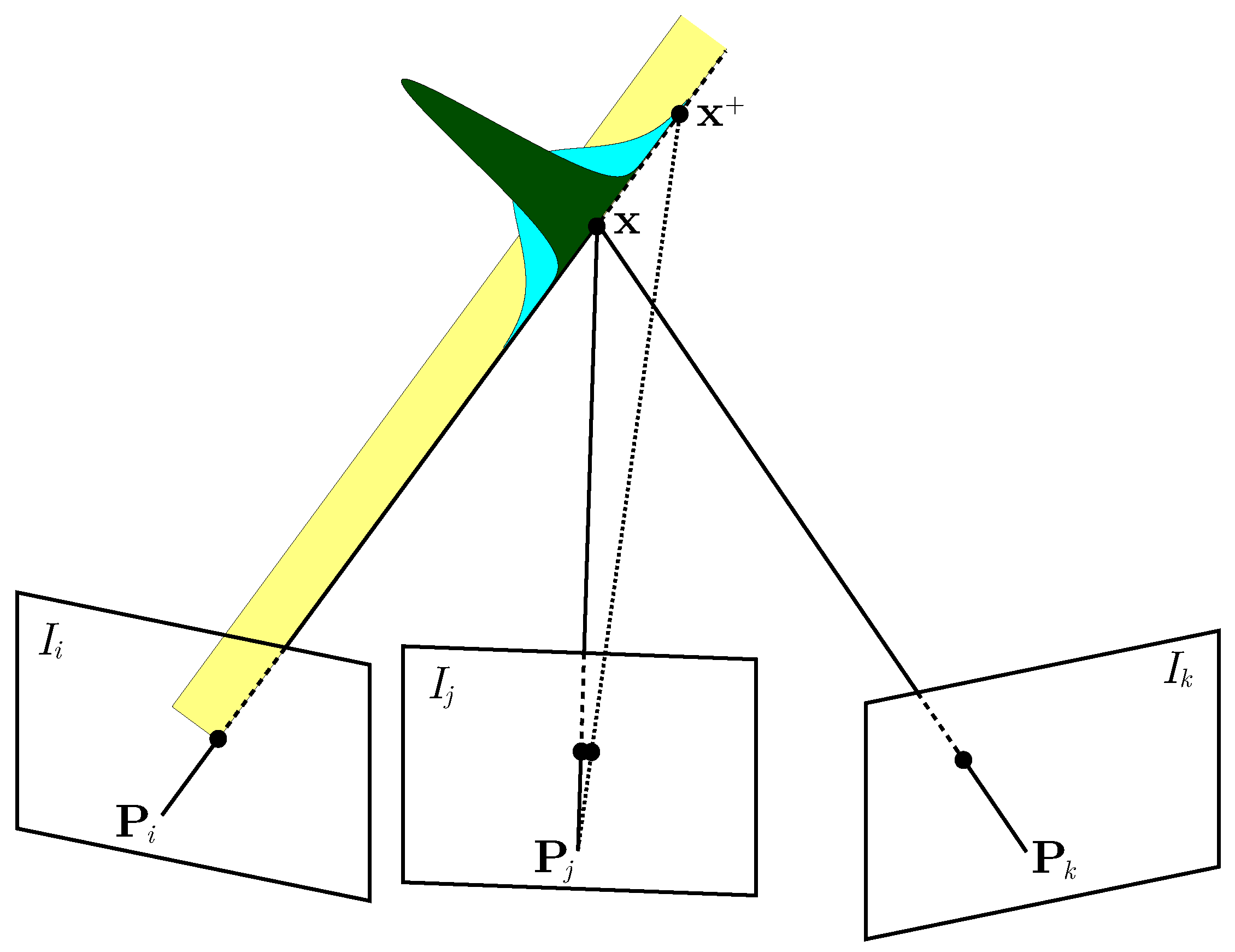
where is obtained by back-projecting the uncertainty of measuring the point in the image plane from image . Figure 3 shows an illustration of the estimation.
Following the derivation of Pizzoli et al. [37], we compute the norm of from the two angles and and the base vector (see Figure 3). To compute these angles, we first need to define the direction of the 3D point from , which is defined as
and can directly be obtained given a calibrated camera. The vector from the second projection center to the 3D point is , exploiting the base vector between both camera. This allows us to define the angle between the base vector and the direction as
as well as the angle between the base vector and :
Under the assumption that we can localize a point in an image with a standard deviation of , we define the angle , which is defined through plus the uncertainty of localizing the point in the image mapped into the space of directions:
where f is the focal length of the camera. Typical feature points can be computed with an uncertainty of 0.3 px to 1 px. In our current implementation, we use a constant uncertainty of 1 px.
As three angles within a triangle need to sum to , we can compute the third angle
and, finally, , which, in turn, is used to compute according to Equation (6):
In practice, we need two views of a 3D point in order to obtain a Gaussian estimate. The uncertainty of the resulting Gaussian directly depends on the angle . The closer approaches 90, the larger the uncertainty reduction.
3.4. Approximating the Information Gain
The main goal of our approach is to find the viewpoint that best reduces the uncertainty in the beliefs about all the points. This uncertainty reduction is given through the expected change in entropy. Thus, the mutual information for a Gaussian point estimate turns into
where refers to the observations obtained at the camera location , while and (computed using Equation (6)) are respectively the current uncertainty of point from view and the estimated uncertainty of the same point from view .
As a result of Equation (13), the expected uncertainty reduction that results from a new image depends on the current uncertainty of the point estimate and on the measurement uncertainty, which itself depends on the geometric configuration of the new viewpoint with respect to the previous viewpoints.
3.5. Combining Information from Multiple Measurements
Starting from the formulation of the measurement uncertainty between two images, we can extend it to multiple images. Intuitively, the more views we add, the smaller the uncertainty becomes, i.e., any new observation of the point reduces its uncertainty, which is the main goal of our exploration strategy. Figure 4 shows how adding a third image reduces the uncertainty of the measured depth of a 3D point. If the point is seen by a single view of a monocular camera, we can compute the direction of the point, but not its depth. Therefore, the uncertainty is represented by a uniform distribution (shown in yellow in Figure 4). After the second view is obtained (or if a stereo camera is used), the uncertainty of the depth is normally distributed and can be obtained as explained in Section 3.3 (see the cyan distribution in Figure 4). From the third view on, the uncertainty is further reduced (see the dark green Gaussian in Figure 4 for an example).
As the correlation between the measurements is unknown, to combine the information from a new image with all the previous ones and compute the total uncertainty, we use the covariance intersection algorithm. Given two distributions of means , and covariance matrices , it is possible to combine them in a third distribution of mean and covariance matrix , computed as
where is a weighting parameter obtained typically by minimizing the determinant or the trace of . To compute , we adopt the closed-form solution proposed by [38]. We approximate the distribution resulting from two images to be univariate, assuming the uncertainty only in the depth of the point seen from the first image, which in turn is assumed without uncertainty. Note that, to reduce the computational load, we compute the covariance intersection only between each new view and the first 10 from which the point has been seen.
3.6. Storing Information
To store the map of the volume to explore (i.e., the portion of the 3D space contained into the bounding box), we discretize it into voxels. For each voxel, we store the total uncertainty of the portion of space inside of it, as well as the viewpoints from which it has been observed. Note that we treat all the points in one voxel alike, i.e., we compute the expected uncertainty reduction per voxel only. Furthermore, as it is typical for occupancy grids, we assume each voxel independent from the others, therefore the total entropy is the sum of the entropy of each voxel. Voxels that are still unexplored have the maximum uncertainty, as no information exists about the state of the cell.
Each time the algorithm needs to choose a new viewpoint, it computes the total expected information gain of each candidate viewpoint by casting rays from that point and summing the expected information gain of all the voxels hit by the rays. Note that, since we acquire images at a constant frame rate, for each candidate viewpoint, we evaluate the information gain for all the intermediate images, by subsampling a computed path between the current position and the possible next one. When a new observation is obtained, we update the uncertainty stored in each voxel seen by the new image. We efficiently store the voxelized map using octrees with the C++ library Octomap [39]. This library can represent voxels with three states (occupied, free and unknown) in an occupancy grid. The API of Octomap allows for automatically updating the states of the voxels by using ray casting, given a depth image and the sensor’s pose. In our implementation, we use a maximum resolution of 0.125 m, as we discretize the space into voxels with a size of 0.5 m × 0.5 m × 0.5 m.
3.7. Changes in the Direction of Flight
As we mentioned in Section 3.1, the action of actually recording the next measurement has a cost, represented by the second term of Equation (4). We define this cost by taking into account the particular needs of an exploration algorithm for MAVs, as explained in this section and in the following one. A key problem of using autonomous MAVs is that, in most countries, a human operator is required to supervise the mission at all times, in order to intervene in case of malfunction or other emergencies. To this purpose, it is helpful if the operator is able to predict the trajectory of the robot, so that he or she can promptly take control of the MAV if it is about to perform a dangerous action. According to our experience, this is substantially simpler if the MAV avoids erratic motion, i.e., its trajectory is short and avoids abrupt changes of direction. Our approach achieves such a behavior by using the cost function:
where grows linearly with the length of the path between the current location of the robot and point , while is a function that grows linearly with the maximum change in orientation that must be executed by the MAV along the path.
3.8. Time-Dependent Cost Function
Most available MAVs have a limited battery life. When planning a mission, it is essential to take the expected battery life into account to prevent the drone from crashing and eventually allowing a safe landing at the starting point. We achieve this by adding a time-dependent component to our cost function. Given a user-specified time limit for the mission, the algorithm dynamically computes a critical time value , based on the trajectory needed to move the MAV from the current location to the starting point. In our implementation, this trajectory is computed by a low-level planner [36]. Once the elapsed-time reaches , the algorithm adds the starting point to the list of possible next points and the time-dependent cost function activates. This has the effect of favoring the robot to:
- fly towards the starting point (for landing);
- avoid flying above obstacles to allow for a potential emergency landing; and
- fly closer to the ground to prevent possible impacts if the battery dies.
Note that, since the starting point is now part of the set of candidate next points, the MAV will land on it as soon as it is close enough.
Thus, we extend Equation (16) by adding the time dependent components, and we obtain the new cost function:
where:
- grows linearly with the elapsed time if in the map there are occupied voxels (excluding the ground) in the area below the MAV, it is equal to 0 otherwise;
- grows linearly with the elapsed time and is proportional to the distance between the current position and the starting point;
- grows linearly with the elapsed time and is proportional to the current altitude of the MAV.
These terms can be chosen in different ways. In our implementation, we represent the cost function as a weighted sum of the different terms, where the weights are tuned by hand. The functions , and have dynamic weights that range between and and are computed as:
Table 1 shows the weights that we use in our experiments. Note that, since the robot might still explore unknown space, this approach does not always guarantee its return to the starting point, but the whole process allows the MAV to increase its safety while still maximizing the information gain. The cost function in Equation (17), plugged in Equation (4), contributes together with the information-gain to the utility function we use to select the next-best-view.
4. Experimental Results
The main focus of our exploration algorithm is to select viewpoints for the purpose of an accurate 3D reconstruction of the environment. Therefore, each new viewpoint has the purpose of exploring new voxels and reducing the uncertainty of the already observed ones. Additionally, the selected viewpoints favor the MAV to follow a path free of sharp changes of direction to allow a human operator to predict more easily its trajectory. Furthermore, the algorithm takes the time into account for a safer flight and landing when the robot is about to run out of battery. Finally, our system has to be fast enough for a real-time execution, as the next-best-view is selected online while the MAV is flying.
Our experiments are designed to show the capabilities of our method and specifically to support the key claims we made in the introduction, which are: (i) our approach yields a map with a low uncertainty in the probabilistic model; (ii) it avoids abrupt changes of direction during the flight; (iii) it does not generate a longer path by taking into account the aforementioned aspects; and (iv) it is able to compute the next best viewpoint in real time and online on an exploring system.
We furthermore provide comparisons to two recent state-of-the-art methods: the exploration algorithm based on Proximity Count VI proposed by Isler et al. [40] and the one proposed by Vasquez-Gomez et al. [29]. We used the existing open source implementation by [40] of both the algorithms, while we implemented our approach from scratch using C++ and ROS.
4.1. Experimental Setup
We tested the three approaches with identical settings on a simulated environment, using the V-REP simulator by Coppelia Robotics (Zürich, Switzerland). We set all the parameters for the algorithms to the default values provided by Isler et al. [40], with the exception of the camera calibration, the ray caster resolution (reduced by a factor of 2), and the ray caster range of 20 m.
The robot in our simulation is a quadcopter with a camera mounted on the front and facing downwards with an angle of 45, as typically vision sensors on MAVs are mounted with angles ranging from 0 to 90. The camera has a field-of-view of 86, a resolution of 2040 by 2040 pixels and a constant frame rate of 20 Hz. We assume to know the sensor pose, which, in practice, can be obtained from a SLAM system such as [1], which runs at 100 Hz on an MAV and operates with an uncertainty of few centimeters. As our algorithm is independent of the sensor used (see Section 1), we obtain the depth information directly from the simulator instead of computing it from the images acquired by the camera. In a real case scenario, this information can come, for example, from a structure from a motion algorithm, or from a stereo camera.
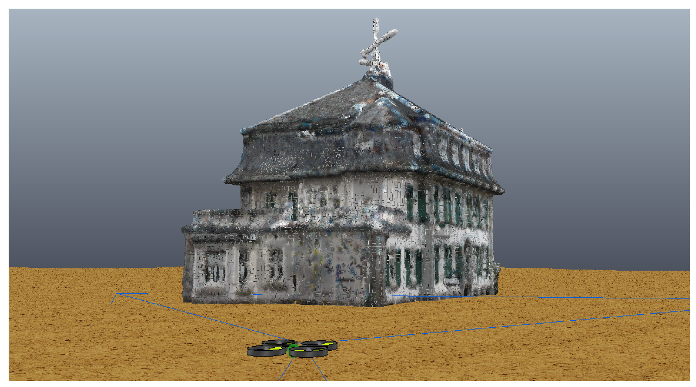
As the object to explore, we selected a building at the University of Bonn called Frankenforst (Figure 1a), and we imported in the virtual scene a 3D model of such building obtained from terrestrial laser scans (see Figure 5). We specified a bounding box around the building with a size of 29 m × 32 m × 25 m, which delimits the volume to explore. As starting locations for the MAV, we sampled 10 locations equally spaced on a circle on the ground around the building. We performed every test 10 times, with the robot starting from each of these 10 locations, performing a vertical take-off and then starting the exploration mission.
During the execution of our algorithm, every time a new viewpoint had to be selected, we recomputed the hull representing the action space of the robot at a distance of 5 m from the occupied voxels in the map, and we sampled 100 points on it (see Section 3.2). Note that, for the comparison with [29,40], we disabled our time-dependent cost function and introduced a boolean cost function in the other two algorithms to prevent collisions, as the implementation by [40] does not provide a functioning collision avoidance system. We stopped the three algorithms after 40 viewpoints were approached.
4.2. Precision of the Reconstruction
The first evaluation is designed to support the claim that our approach selects viewpoints that increase the number of observed voxels and reduce the uncertainty of the already observed ones. We evaluate the precision of the 3D reconstruction by measuring the uncertainty of the observations obtained from the camera, using the formulation explained in Section 3.3.
Figure 6a shows the path and the map resulting from the execution of our algorithm after 40 computed viewpoints. Each voxel is colored according to the total uncertainty of the points it contains, with the colormap shown in Figure 6. For an accurate 3D reconstruction, the uncertainty should be “medium” or lower (from green to yellow in our colormap). The figure shows qualitatively that most of the voxels in the map have an uncertainty lower than the acceptable value, i.e., it is possible to accurately reconstruct the building in 3D from the acquired images.
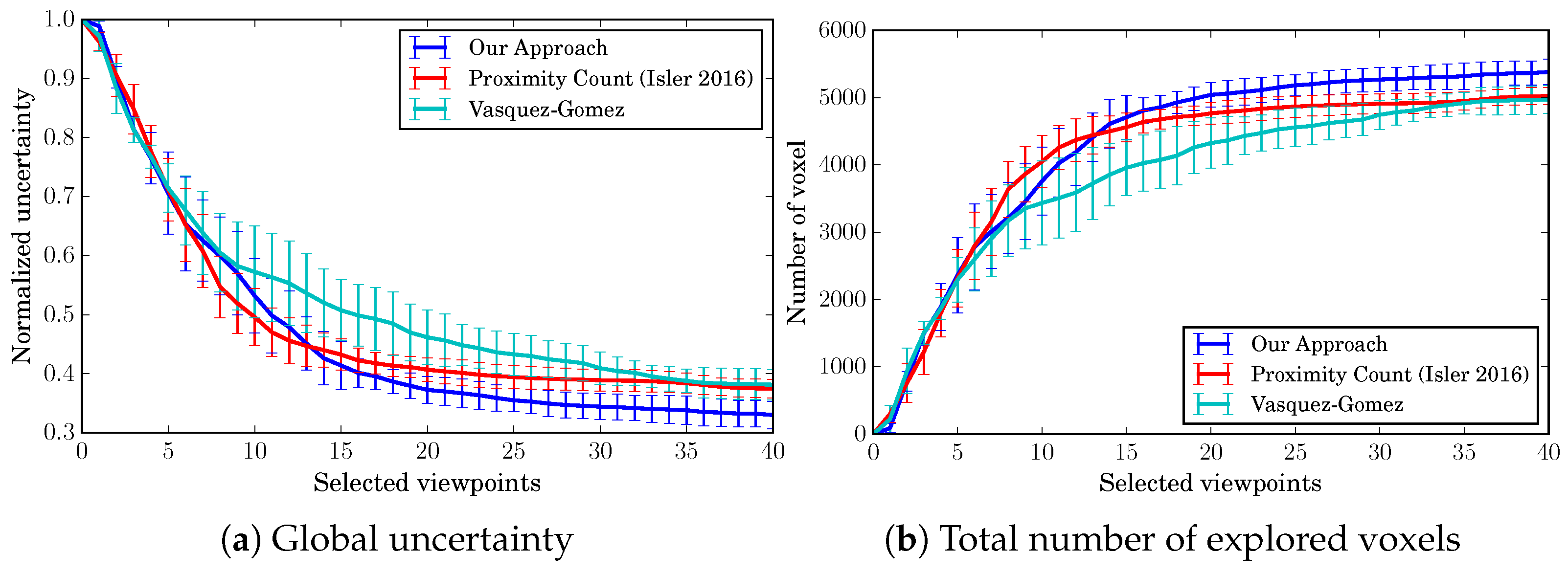
As a quantitative evaluation, Figure 7 shows how the normalized global uncertainty and the total number of explored voxel in the map evolve during the exploration. The figure shows mean values and standard deviations over our 10 tests described above. We define the normalized global uncertainty as:
where is the uncertainty of the i-th voxel, N is the number of voxels in the map and is the maximum possible uncertainty, i.e., the sum of the uncertainty of every voxel before the exploration starts. At the beginning of the exploration, every voxel has infinite uncertainty, simulated in practice by a large fixed value (in our implementation 10,000,000). Note that the metric we use depends on this maximum value. Therefore, we set the value identically for all algorithms so that the obtained performance measure allows for a fair comparison between the approaches. Moreover, since we use an octree to store the map, to compute this measure, we expand the tree to obtain all the voxels on the same level, i.e., we convert the map to a simple voxel grid for this evaluation. In both Figure 7a,b, the three algorithms show similar performances, with a slight advantage of our approach. Moreover, by looking at the std. deviations, it is clear that none of the algorithms are affected by the starting point of the flight, and, in general, the results are consistent among different flights.
4.3. Path Smoothness
A particular focus of our approach is the shape of the flight path. From our experience, a human supervisor, who is required by law in several countries, can more easily predict the trajectory of the MAV if it is free of abrupt turns. Our second evaluation supports our second claim, namely that our approach is able to select viewpoints that favor a path that avoids sharp changes of direction. This is qualitatively visible in Figure 6, where the path chosen by our approach, compared to the one by Vasquez-Gomez et al. [29], is fairly regular and basically performs larger turns only if the model requires it.
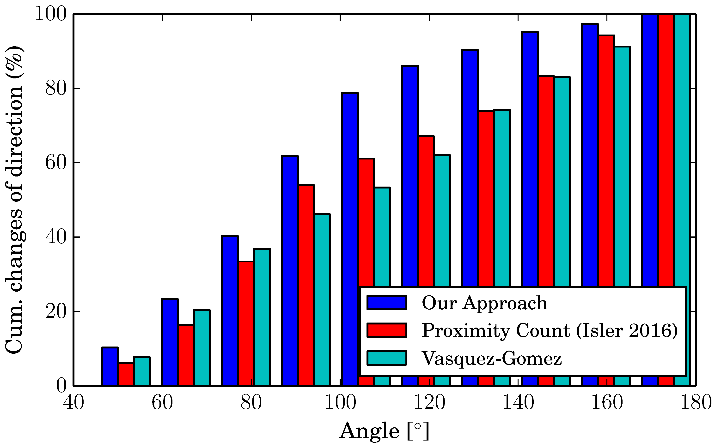
To compare this aspect between the different algorithms, we considered the angles of each change of direction and counted them. The histogram in Figure 8 shows the cumulative percentage of changes of direction for angles between 40 and 180, divided into 10 intervals. As the figure shows, the other approaches have no preference at all when choosing the direction to take for the next viewpoint (the bars have a linear trend). Our algorithm, on the other hand, chooses in 80% of the cases a point at an angle below 100, thanks to our utility function, which takes this measure into account.
4.4. Path Length
An important aspect of an exploration algorithm is the length of the path that the robot needs to follow to complete the procedure. In this section, we support our third claim, i.e., our algorithm has performances aligned to the current state-of-the-art in terms of path length, despite its utility function, which is designed for a more predictable path.
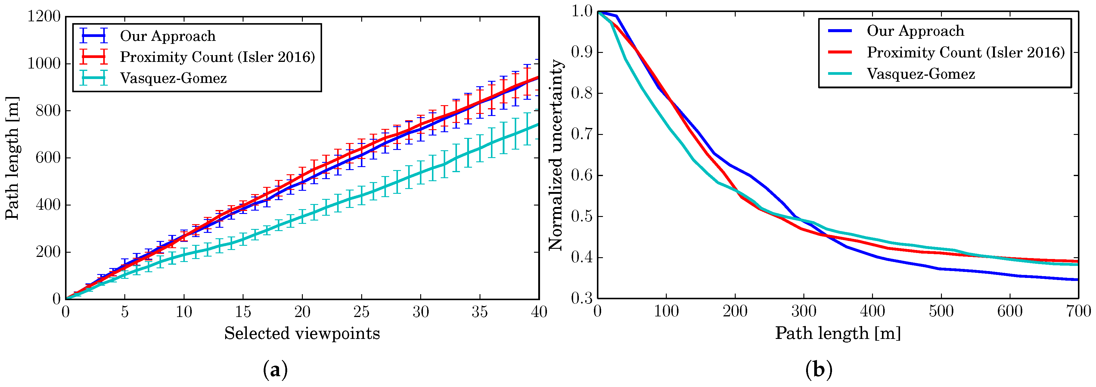
Figure 9a shows the total path length after approaching each next viewpoint. The best performing algorithm in this case is the one by Vasquez-Gomez et al., due to its utility function, specifically designed to create overlaps between the views. Our approach, instead, is aligned to the one by Isler et al. We also consider the uncertainty reduction and relate it to the travelled distance (see Figure 9b). The plot shows that, after 350 the three algorithms show a similar performance. Therefore, the longer distance between the single viewpoints is compensated by a better reduction of the uncertainty. Thus, we can conclude that our strategy to select viewpoints for a more regular path does not substantially affect the total length.
4.5. Execution Time
The final comparison we make is between the execution time of the three approaches. Table 2 shows the average time spent to compute the next viewpoint on a single core of a regular Intel Core i7 CPU. In our tests, our approach performed about five times faster. In addition to that, Figure 10 shows the uncertainty against the elapsed time. As can be seen, our approach reduces the uncertainty faster while the time elapses and it is fast enough to be used in real time.
4.6. Time-Dependent Cost Function
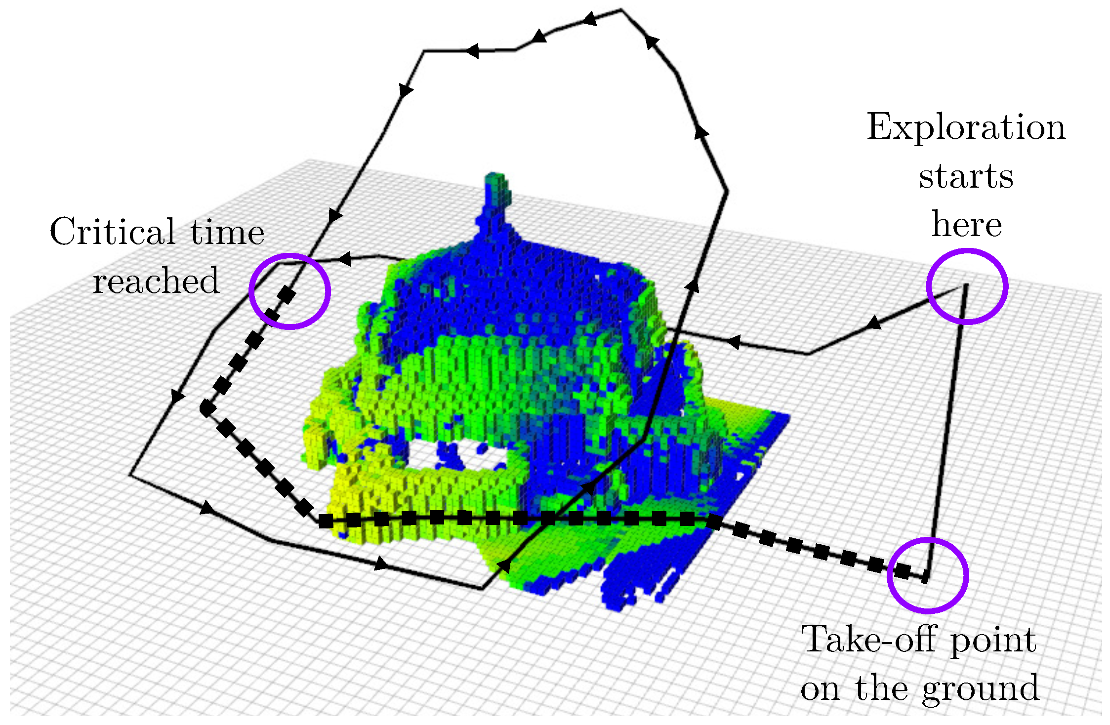
The last aspect of our algorithm is its capability of selecting viewpoints that favor the MAV to move back to its starting point before it runs out of battery, while still taking into account the information gain expected from the new viewpoints. Figure 11 shows a path computed with a time limit. At first, the algorithm explores normally the building (black continuous path), but, when the critical time is reached, as shown by the square markers, the MAV flies towards the starting point, while still trying to reduce the uncertainty, keeping a low altitude and avoiding flying above obstacles.
4.7. Real World Experiment
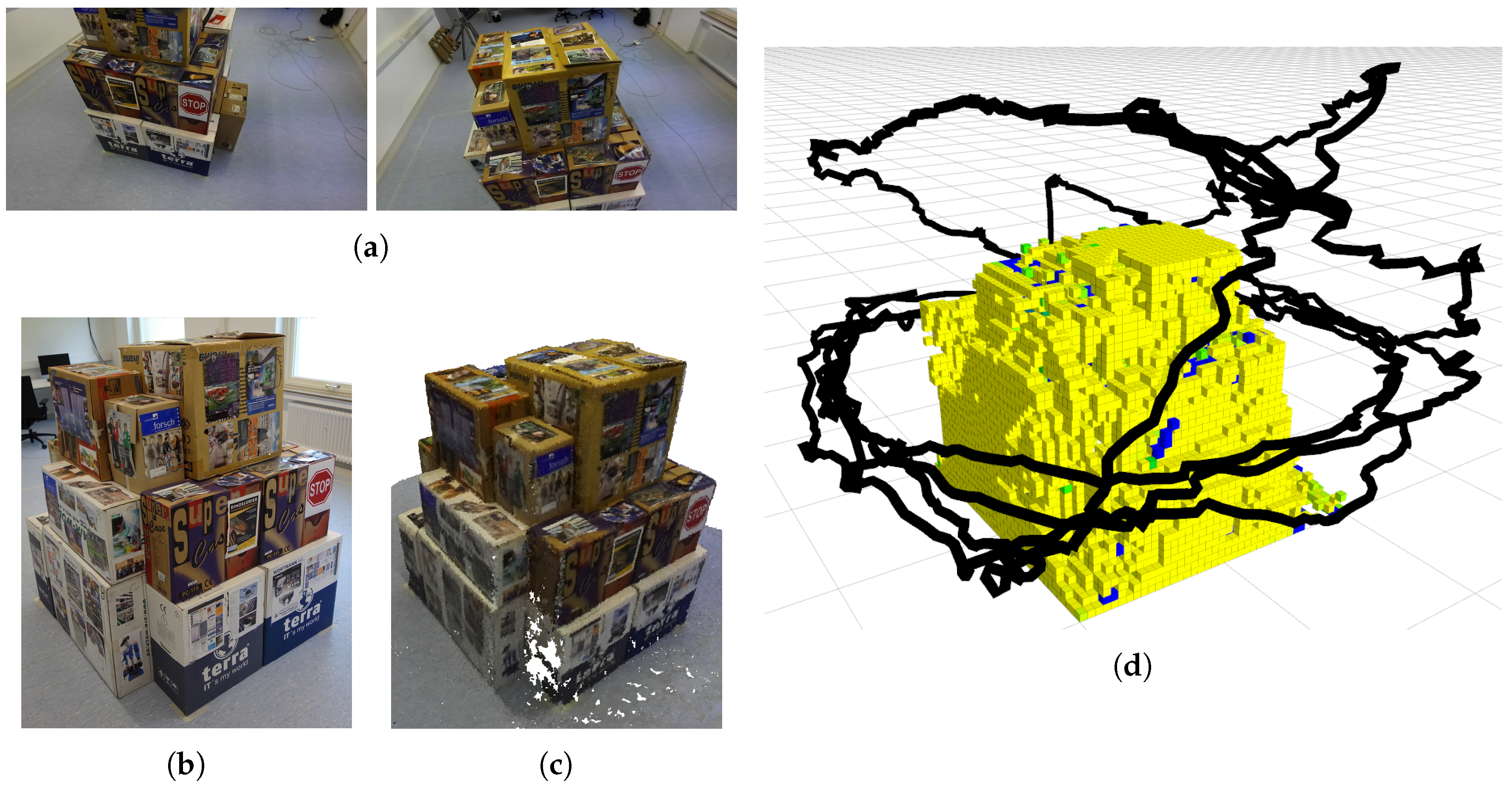
We finally provide a test of our algorithm in the real world. We created a test environment composed by a structure of boxes in an indoor scene (see Figure 12b). The sensor we use is a ZED stereo camera by Stereolabs (San Francisco, CA, USA), which provides, out-of-the-box and in real time, the depth information computed from the stereo images. We run our algorithm with similar settings as the simulated tests, eventually scaled to the size of the new environment. In particular, we used the same weights for the cost function (see Table 1) and sampled the same number of candidate next viewpoints at each iteration (100), but we increased the map resolution by reducing the voxel size to 0.05 m per side, and we reduced the distance of the hull (representing the action space of the robot) from the occupied voxels in the map to 1 m. Figure 12a shows some frames acquired by the camera during the execution of the algorithm. Figure 12d shows the final map of the structure and the actual trajectory of the camera, after 60 computed viewpoints.
To test the use of our algorithm for a real 3D reconstruction case, we used the recorded image sequence as input for an offline, out-of-the-box dense reconstruction approach. Figure 12c shows the final dense pointcloud. Note that no contribution for the dense reconstruction approach itself is claimed here.
5. Conclusions
In this paper, we presented a novel approach for vision based autonomous exploration on MAVs. Our approach iteratively samples candidate viewpoints and greedily selects the optimal one using a utility function. This function takes into account the expected information gain from the new view, the distance from the current position to the new point and the change of direction of motion. Additionally, a time-dependent component in the function allows for a safer flight and landing when the MAV is about to run out of battery. We implemented our approach in C++ and ROS and evaluated it in simulated and real environments. We compared the approach to two state-of-the-art methods and our experiments suggest that our algorithm allows for a precise exploration while flying on a trajectory comparably free of abrupt changes of direction of motion, without sacrificing the path length and in an online, real-time fashion.
Acknowledgments
This work has partly been supported by the Deutsche Forschungsgemeinschaft (DFG) under the grant number FOR 1505: Mapping on Demand.
Author Contributions
The actual implementation of the approach was done by Emanuele Palazzolo. The design of the approach, the design and execution of experiments, and the paper writing was done in equal share. Cyrill Stachniss supplied the required infrastructure.
Conflicts of Interest
The authors declare no conflict of interest. The founding sponsors had no role in the design of the study; in the collection, analyses, or interpretation of data; in the writing of the manuscript, and in the decision to publish the results.
References
- Schneider, J.; Eling, C.; Klingbeil, L.; Kuhlmann, H.; Förstner, W.; Stachniss, C. Fast and Effective Online Pose Estimation and Mapping for UAVs. In Proceedings of the 2016 IEEE International Conference on Robotics and Automation (ICRA), Stockholm, Sweden, 16–21 May 2016. [Google Scholar]
- Palazzolo, E.; Stachniss, C. Information-Driven Autonomous Exploration for a Vision-Based MAV. ISPRS Ann. Photogramm. Remote Sens. Spat. Inf. Sci. 2017, IV-2/W3, 59–66. [Google Scholar] [CrossRef]
- Yamauchi, B. A frontier-based approach for autonomous exploration. In Proceedings of the IEEE International Symposium on Computational Intelligence in Robotics and Automation, Monterey, CA, USA, 10–11 July 1997; pp. 146–151. [Google Scholar]
- Bourgault, F.; Makarenko, A.A.; Williams, S.B.; Grocholsky, B.; Durrant-Whyte, H.F. Information based adaptive robotic exploration. In Proceedings of the 2002 IEEE/RSJ International Conference on Intelligent Robots and Systems (IROS), Lausanne, Switzerland, 30 September–4 October 2002; Volume 1, pp. 540–545. [Google Scholar]
- Stachniss, C.; Grisetti, G.; Burgard, W. Information Gain-based Exploration Using Rao-Blackwellized Particle Filters. In Proceedings of the Robotics: Science and Systems (RSS), Cambridge, MA, USA, 8–11 June 2005; pp. 65–72. [Google Scholar]
- Ström, D.P.; Nenci, F.; Stachniss, C. Predictive Exploration Considering Previously Mapped Environments. In Proceedings of the IEEE International Conference on Robotics and Automation (ICRA), Seattle, WA, USA, 26–30 May 2015. [Google Scholar]
- Fraundorfer, F.; Heng, L.; Honegger, D.; Lee, G.H.; Meier, L.; Tanskanen, P.; Pollefeys, M. Vision-based autonomous mapping and exploration using a quadrotor MAV. In Proceedings of the 2012 IEEE/RSJ International Conference on Intelligent Robots and Systems (IROS), Vilamoura, Portugal, 7–12 October 2012; pp. 4557–4564. [Google Scholar]
- Shen, S.; Michael, N.; Kumar, V. Autonomous indoor 3D exploration with a micro-aerial vehicle. In Proceedings of the IEEE International Conference on Robotics and Automation (ICRA), Saint Paul, MN, USA, 14–18 May 2012; pp. 9–15. [Google Scholar]
- Cieslewski, T.; Kaufmann, E.; Scaramuzza, D. Rapid Exploration with Multi-Rotors: A Frontier Selection Method for High Speed Flight. In Proceedings of the IEEE/RSJ International Conference on Intelligent Robots and Systems (IROS), Vancouver, BC, Canada, 24–28 September 2017. [Google Scholar]
- Bircher, A.; Kamel, M.; Alexis, K.; Oleynikova, H.; Siegwart, R. Receding Horizon “Next-Best-View” Planner for 3D Exploration. In Proceedings of the 2016 IEEE International Conference on Robotics and Automation (ICRA), Stockholm, Sweden, 16–21 May 2016. [Google Scholar]
- Aloimonos, J.; Weiss, I.; Bandyopadhyay, A. Active vision. Int. J. Comput. Vis. (IJCV) 1988, 1, 333–356. [Google Scholar] [CrossRef]
- Bajcsy, R. Active perception. Proc. IEEE 1988, 76, 966–1005. [Google Scholar] [CrossRef]
- Scott, W.; Roth, G.; Rivest, J.F. View planning for automated 3D object reconstruction inspection. ACM Comput. Surv. 2003, 35, 64–96. [Google Scholar] [CrossRef]
- Hoppe, C.; Klopschitz, M.; Rumpler, M.; Wendel, A.; Kluckner, S.; Bischof, H.; Reitmayr, G. Online Feedback for Structure-from-Motion Image Acquisition. In Proceedings of the British Machine Vision Conference (BMVC), Guildford, UK, 3–7 September 2012; pp. 70.1–70.12. [Google Scholar]
- Dunn, E.; Frahm, J.M. Next Best View Planning for Active Model Improvement. In Proceedings of the British Machine Vision Conference (BMVC), London, UK, 7–10 September 2009; pp. 1–11. [Google Scholar]
- Kriegel, S.; Bodenmüller, T.; Suppa, M.; Hirzinger, G. A surface-based next-best-view approach for automated 3D model completion of unknown objects. In Proceedings of the 2011 IEEE International Conference on Robotics & Automation (ICRA), Shanghai, China, 9–13 May 2011; pp. 4869–4874. [Google Scholar]
- Pito, R. A solution to the next best view problem for automated surface acquisition. IEEE Trans. Pattern Anal. Mach. Intell. (TPAMI) 1999, 21, 1016–1030. [Google Scholar] [CrossRef]
- Quin, P.; Paul, G.; Alempijevic, A.; Liu, D.; Dissanayake, G. Efficient neighbourhood-based information gain approach for exploration of complex 3D environments. In Proceedings of the 2013 IEEE International Conference on Robotics & Automation (ICRA), Karlsruhe, Germany, 6–10 May 2013; pp. 1343–1348. [Google Scholar]
- Krainin, M.; Curless, B.; Fox, D. Autonomous generation of complete 3D object models using next best view manipulation planning. In Proceedings of the IEEE International Conference on Robotics & Automation (ICRA), Shanghai, China, 9–13 May 2011; pp. 5031–5037. [Google Scholar]
- Potthast, C.; Sukhatme, G. A probabilistic framework for next best view estimation in a cluttered environment. J. Vis. Commun. Image Represent. (JVCIR) 2014, 25, 148–164. [Google Scholar] [CrossRef]
- Trummer, M.; Munkelt, C.; Denzler, J. Online next-best-view planning for accuracy optimization using an extended e-criterion. In Proceedings of the 2010 20th International Conference on Pattern Recognition (ICPR), Istanbul, Turkey, 23–26 August 2010; pp. 1642–1645. [Google Scholar]
- Bircher, A.; Alexis, K.; Burri, M.; Oettershagen, P.; Omari, S.; Mantel, T.; Siegwart, R. Structural inspection path planning via iterative viewpoint resampling with application to aerial robotics. In Proceedings of the 2015 IEEE International Conference on Robotics & Automation (ICRA), Seattle, WA, USA, 26–30 May 2015; pp. 6423–6430. [Google Scholar]
- Schmid, K.; Hirschmüller, H.; Dömel, A.; Grixa, I.; Suppa, M.; Hirzinger, G. View planning for multi-view stereo 3d reconstruction using an autonomous multicopter. J. Intell. Robot. Syst. (JIRS) 2012, 65, 309–323. [Google Scholar] [CrossRef]
- Shade, R.; Newman, P. Choosing where to go: Complete 3D exploration with stereo. In Proceedings of the IEEE International Conference on Robotics & Automation (ICRA), Shanghai, China, 9–13 May 2011; pp. 2806–2811. [Google Scholar]
- Haner, S.; Heyden, A. Optimal view path planning for visual SLAM. In Proceedings of the Scandinavian Conference on Image Analysis, Ystad, Sweden, 23–25 May 2011; pp. 370–380. [Google Scholar]
- Mostegel, C.; Wendel, A.; Bischof, H. Active monocular localization: Towards autonomous monocular exploration for multirotor MAVs. In Proceedings of the 2014 IEEE International Conference on Robotics & Automation (ICRA), Hong Kong, China, 31 May–7 June 2014; pp. 3848–3855. [Google Scholar]
- Sadat, S.A.; Chutskoff, K.; Jungic, D.; Wawerla, J.; Vaughan, R. Feature-rich path planning for robust navigation of MAVs with mono-SLAM. In Proceedings of the IEEE International Conference on Robotics & Automation (ICRA), Hong Kong, China, 31 May–7 June 2014; pp. 3870–3875. [Google Scholar]
- Delmerico, J.; Isler, S.; Sabzevari, R.; Scaramuzza, D. A comparison of volumetric information gain metrics for active 3D object reconstruction. Auton. Robot. 2018, 42, 197–208. [Google Scholar] [CrossRef]
- Vasquez-Gomez, J.; Sucar, L.; Murrieta-Cid, R.; Lopez-Damian, E. Volumetric next-best-view planning for 3d object reconstruction with positioning error. Int. J. Adv. Robot. Syst. 2014, 11, 1–13. [Google Scholar] [CrossRef]
- Forster, C.; Pizzoli, M.; Scaramuzza, D. Appearance-based Active, Monocular, Dense Reconstruction for Micro Aerial Vehicle. In Proceedings of the Robotics: Science and Systems (RSS), Berkeley, CA, USA, 12–16 July 2014. [Google Scholar]
- Bai, S.; Chen, F.; Englot, B. Toward Autonomous Mapping and Exploration for Mobile Robots through Deep Supervised Learning. In Proceedings of the 2017 IEEE/RSJ International Conference on Intelligent Robots and Systems (IROS), Vancouver, BC, Canada, 24–28 September 2017. [Google Scholar]
- Charrow, B.; Kahn, G.; Patil, S.; Liu, S.; Goldberg, K.; Abbeel, P.; Michael, N.; Kumar, V. Information-theoretic planning with trajectory optimization for dense 3d mapping. In Proceedings of the Robotics: Science and Systems (RSS), Rome, Italy, 13–17 July 2015. [Google Scholar]
- Freundlich, C.; Mordohai, P.; Zavlanos, M.M. A hybrid control approach to the next-best-view problem using stereo vision. In Proceedings of the IEEE International Conference on Robotics & Automation (ICRA), Karlsruhe, Germany, 6–10 May 2013; pp. 4493–4498. [Google Scholar]
- Atanasov, N.; Le Ny, J.; Daniilidis, K.; Pappas, G.J. Decentralized active information acquisition: Theory and application to multi-robot SLAM. In Proceedings of the IEEE International Conference on Robotics & Automation (ICRA), Seattle, WA, USA, 26–30 May 2015; pp. 4775–4782. [Google Scholar]
- Strasdat, H.; Stachniss, C.; Burgard, W. Which Landmark is Useful? Learning Selection Policies for Navigation in Unknown Environments. In Proceedings of the IEEE International Conference on Robotics & Automation (ICRA), Kobe, Japan, 12–17 May 2009. [Google Scholar]
- Nieuwenhuisen, M.; Behnke, S. Layered mission and path planning for MAV navigation with partial environment knowledge. In Intelligent Autonomous Systems 13; Springer: Berlin, Germany, 2016; pp. 307–319. [Google Scholar]
- Pizzoli, M.; Forster, C.; Scaramuzza, D. REMODE: Probabilistic, monocular dense reconstruction in real time. In Proceedings of the IEEE International Conference on Robotics & Automation (ICRA), Hong Kong, China, 31 May–7 June 2014; pp. 2609–2616. [Google Scholar]
- Reinhardt, M.; Noack, B.; Hanebeck, U. Closed-form optimization of covariance intersection for low-dimensional matrices. In Proceedings of the 2012 15th International Conference on Information Fusion, Singapore, 9–12 July 2012; pp. 1891–1896. [Google Scholar]
- Hornung, A.; Wurm, K.; Bennewitz, M.; Stachniss, C.; Burgard, W. OctoMap: An Efficient Probabilistic 3D Mapping Framework Based on Octrees. Auton. Robot. 2013, 34, 189–206. [Google Scholar] [CrossRef]
- Isler, S.; Sabzevari, R.; Delmerico, J.; Scaramuzza, D. An Information Gain Formulation for Active Volumetric 3D Reconstruction. In Proceedings of the IEEE International Conference on Robotics & Automation (ICRA), Stockholm, Sweden, 16–21 May 2016. [Google Scholar]
Figure 1.
Given a scene containing an object of interest (a); our algorithm computes the best viewpoints to efficiently map the environment (b).
Figure 1.
Given a scene containing an object of interest (a); our algorithm computes the best viewpoints to efficiently map the environment (b).
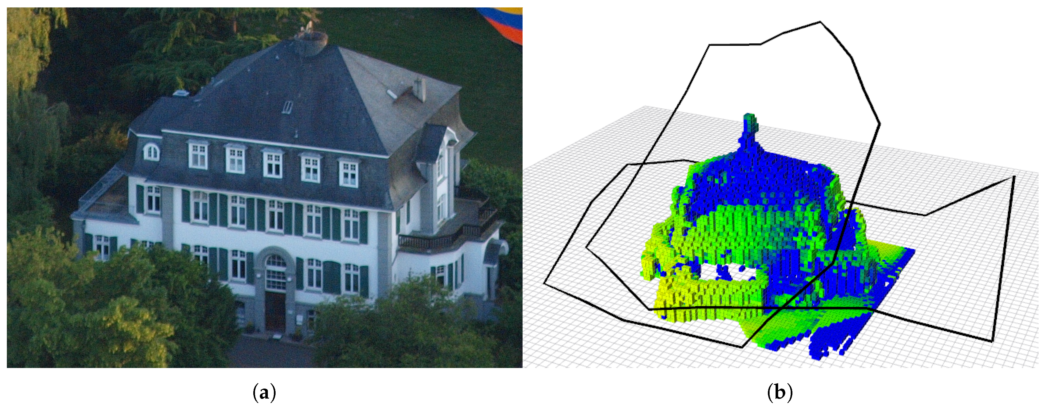
Figure 2.
(a) the MAV’s movements are constrained to a hull (red dotted line) that is initially built around the user-specified bounding box (blue area delimited by dashed green border); (b) the hull is then adapted according to the new explored (yellow squares) and unknown (gray squares) voxels.
Figure 2.
(a) the MAV’s movements are constrained to a hull (red dotted line) that is initially built around the user-specified bounding box (blue area delimited by dashed green border); (b) the hull is then adapted according to the new explored (yellow squares) and unknown (gray squares) voxels.
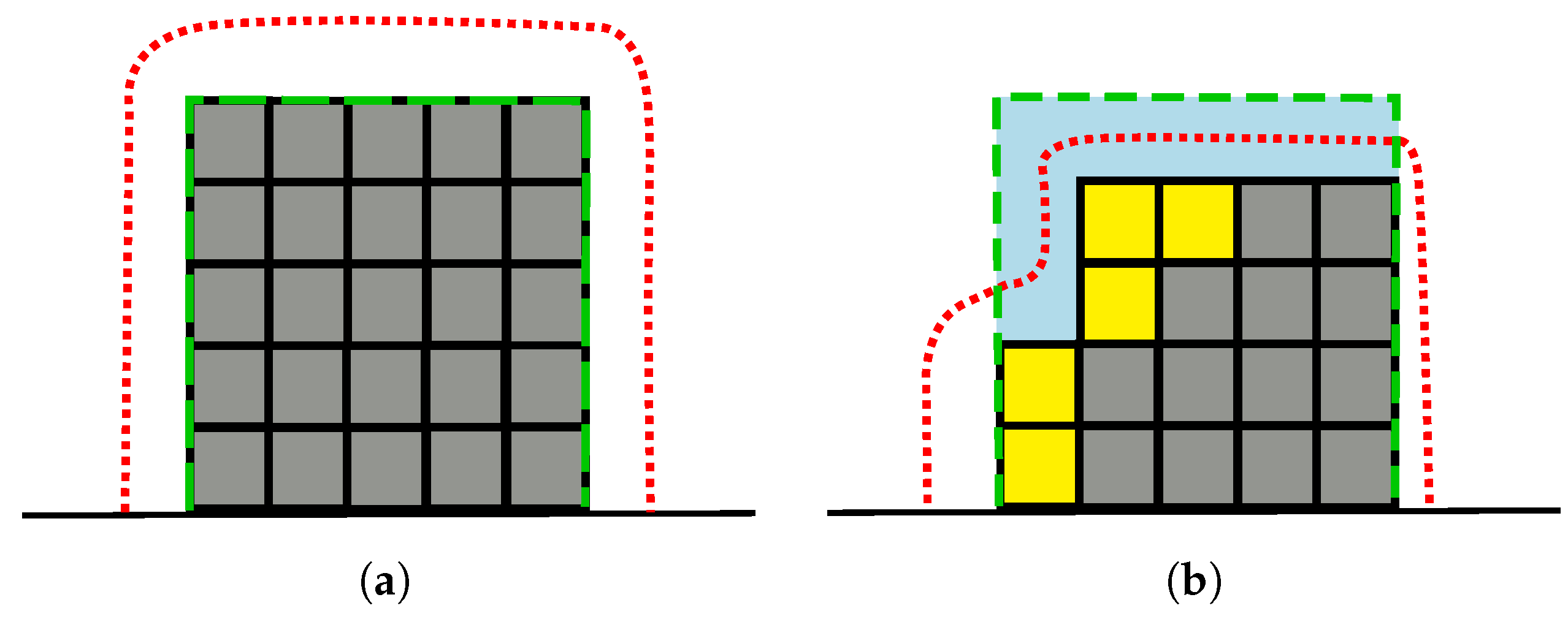
Figure 3.
The measurement uncertainty of a depth point from two images can be computed through and as elaborated in the REMODE approach [37] for 3D reconstruction from monocular images.
Figure 3.
The measurement uncertainty of a depth point from two images can be computed through and as elaborated in the REMODE approach [37] for 3D reconstruction from monocular images.
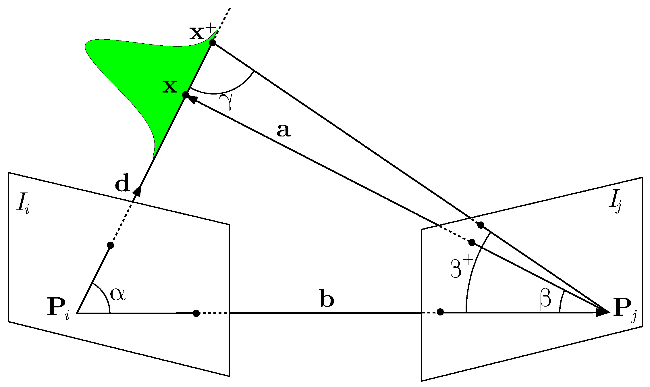
Figure 4.
Illustration of the reduction of the uncertainty in the estimate about the 3D point location given a third image.
Figure 4.
Illustration of the reduction of the uncertainty in the estimate about the 3D point location given a third image.

Figure 5.
Simulated environment in V-REP simulator. The scene contains the Frankenforst building and the MAV.
Figure 5.
Simulated environment in V-REP simulator. The scene contains the Frankenforst building and the MAV.

Figure 6.
Result of the execution of our algorithm (a) and the approach by Vasquez-Gomez et al. [29] (b) after 40 computed viewpoints. The black line represents the trajectory and the model in the center is the result of the mapping. The voxels are colored according to their uncertainty.
Figure 6.
Result of the execution of our algorithm (a) and the approach by Vasquez-Gomez et al. [29] (b) after 40 computed viewpoints. The black line represents the trajectory and the model in the center is the result of the mapping. The voxels are colored according to their uncertainty.
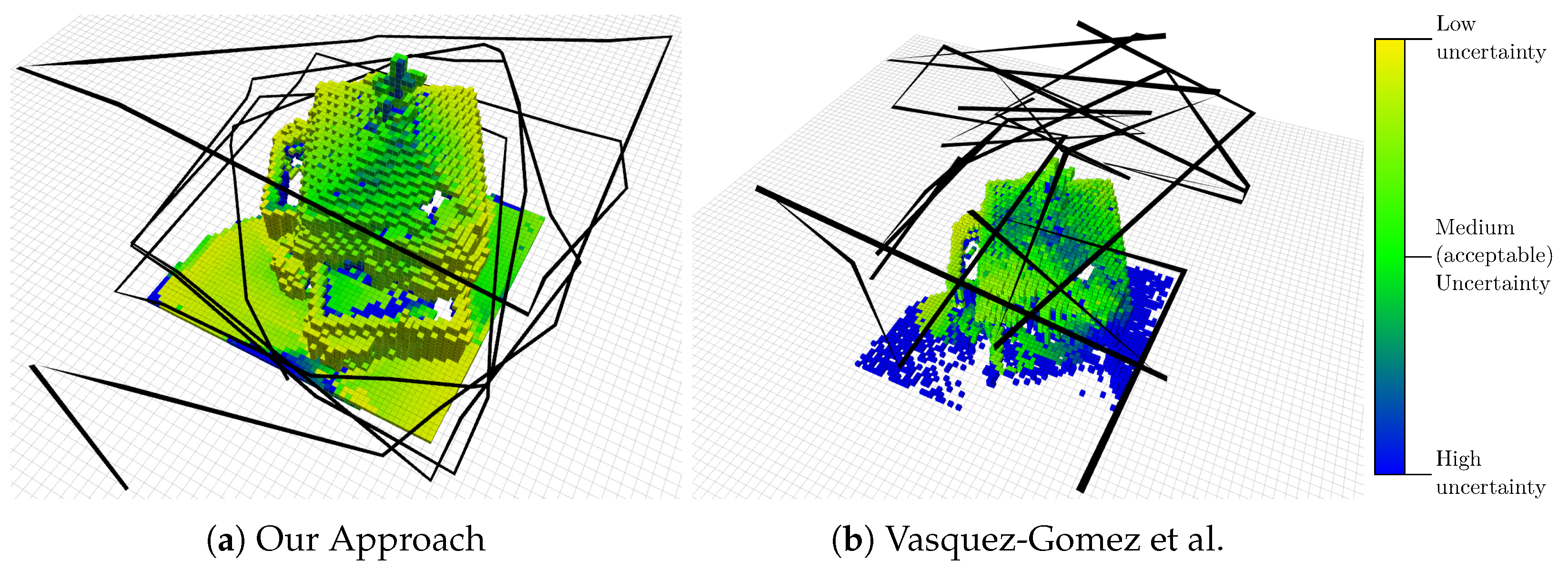
Figure 7.
Quantitative evaluation of the reconstruction quality (mean values and std. deviations). (a) global uncertainty of the map at each selected viewpoint; (b) total number of explored voxels in the map at each selected viewpoint.
Figure 7.
Quantitative evaluation of the reconstruction quality (mean values and std. deviations). (a) global uncertainty of the map at each selected viewpoint; (b) total number of explored voxels in the map at each selected viewpoint.

Figure 8.
Cumulative histogram of the changes of direction.

Figure 9.
(a) path length at each selected viewpoint; (b) map uncertainty versus traveled distance.

Figure 10.
Map uncertainty versus elapsed time.
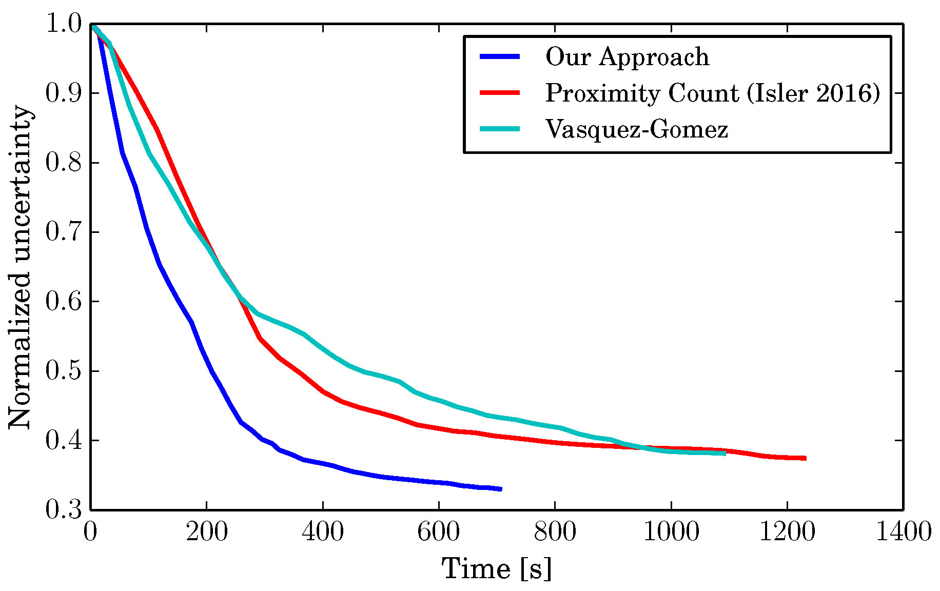
Figure 11.
Path computed with the time-dependent cost function enabled. The square markers represent the path generated after the critical time, which moves the MAV back to the starting point.
Figure 11.
Path computed with the time-dependent cost function enabled. The square markers represent the path generated after the critical time, which moves the MAV back to the starting point.

Figure 12.
Real world experiment: (a) two examples of camera frames; (b) test environment; (c) obtained model; (d) voxel map and followed path.
Figure 12.
Real world experiment: (a) two examples of camera frames; (b) test environment; (c) obtained model; (d) voxel map and followed path.


Table 1.
Weights used in the cost function in our implementation.
| Function | Weight [s] |
|---|---|
| 1000 | |
| 30,000 | |
| , | |
| , 12,000 | |
| , |
Table 2.
Average time and std. deviation to compute a viewpoint with the different algorithms.
| Algorithm | Average Time and Std. Deviation [s] |
|---|---|
| Our algorithm | 1.31 () |
| Proximity count (Isler 2016) | 6.53 () |
| Vasquez-Gomez | 6.58 () |
© 2018 by the authors. Licensee MDPI, Basel, Switzerland. This article is an open access article distributed under the terms and conditions of the Creative Commons Attribution (CC BY) license (http://creativecommons.org/licenses/by/4.0/).
Share and Cite
MDPI and ACS Style
Palazzolo, E.; Stachniss, C. Effective Exploration for MAVs Based on the Expected Information Gain. Drones 2018, 2, 9. https://doi.org/10.3390/drones2010009
AMA Style
Palazzolo E, Stachniss C. Effective Exploration for MAVs Based on the Expected Information Gain. Drones. 2018; 2(1):9. https://doi.org/10.3390/drones2010009
Chicago/Turabian StylePalazzolo, Emanuele, and Cyrill Stachniss. 2018. "Effective Exploration for MAVs Based on the Expected Information Gain" Drones 2, no. 1: 9. https://doi.org/10.3390/drones2010009