Reliability of Cutting Edge Radius Estimator Based on Chip Production Rate for Micro End Milling


1
School for Engineering of Matter, Transport and Energy, Arizona State University, Tempe, AZ 85281, USA
2
Faculty of Polytechnic School, Arizona State University, Mesa, AZ 85212, USA
*
Author to whom correspondence should be addressed.
J. Manuf. Mater. Process. 2019, 3(1), 25; https://doi.org/10.3390/jmmp3010025
Submission received: 18 February 2019
/
Revised: 16 March 2019
/
Accepted: 18 March 2019
/
Published: 20 March 2019
(This article belongs to the Special Issue New Findings and Approaches in Machining Processes)
Abstract
:In this paper, the reliability of a new online cutting edge radius estimator for micro end milling is evaluated. This estimator predicts the cutting edge radius by detecting the drop in the chip production rate as the cutting edge of a micro end mill slips over the workpiece when the minimum chip thickness (MCT) becomes larger than the uncut chip thickness (UCT), thus transitioning from the shearing to the ploughing dominant regime. This study proposes a method of calibrating the cutting edge radius estimator by determining two parameters from training data: a ‘size filtering threshold’ that specifies the smallest-size chip that should be counted, and a ‘drop detection threshold’ that distinguishes the drop in the number of chips at the actual critical feedrate from the number drops at the other feedrates. This study then evaluates the accuracy of the calibrated estimator from testing data for determining the ‘critical feedrate’—the feedrate at which the MCT and UCT will be equal. It is found that the estimator is successful in determining the critical feedrate to within 1 mm/s in 84% of trials.
1. Introduction
As the need for micro-components has grown in various engineering fields, the demand for technology development for micro-manufacturing has increased [1]. In particular, micro milling, one of the micro-machining techniques belonging to micro-manufacturing, has many advantages. It has a lower initial cost than the other micro-manufacturing processes that are based on lithography. Also, it is possible to manufacture small complex 3-D parts, unlike the lithography method which is limited to 2-D or 2.5-D geometry. In addition, it has a relatively wide choice of workpiece materials [2,3,4,5]. Therefore, micro-milling is used in various fields such as automotive, aerospace, and biomedical industry etc. For example, in the biochemical industry, microfluidic chips are manufactured through the micro milling process [6,7,8].
However, the cutting mechanisms for macro-scale milling are not applicable to micro milling due to the “MCT effect”. In conventional milling, the cutting mechanism is dominated by shearing. But, in micro milling, the cutting mechanism is divided into shearing/ploughing by the MCT effect which has a great influence on cutting force, chip production, surface quality, and tool wear [9,10,11]. Additionally, vibration is a more important factor in micro milling since higher spindle speed is needed compared to conventional milling [12,13]. In order to clarify the relationships between the MCT effect, the chip formation, the cutting force, the vibration, the surface quality, and the tool wear in micro-milling, many studies have been conducted.
Since the MCT can be approximated as 30% of the cutting edge radius which depends on the tool wear, the MCT effect is directly related to the tool wear [5,10,14]. In particular, the chip formation in micro milling can be significantly affected by the tool wear. When the cutting edge radius becomes larger as the tool wears, the MCT becomes larger as well. When the MCT becomes larger than the UCT, the chip formation mechanism changes from the shearing regime generating one chip per tooth pass to the ploughing regime generating no chip per tooth pass [9,15,16]. In addition, it has been found that the cutting force increases as the tool wear increases [17,18]. When the cutting edge radius becomes larger due to the tool wear, the ploughing becomes dominant in the cutting mechanism. Then, the UCT would be accumulated. As the UCT accumulates, the cutting force accumulates until the UCT becomes larger than the MCT [19]. Moreover, the cutting force is also closely related to the vibration since the high variation in the cutting force causes excessive vibrations resulting in the increase of the tool wear rate [20]. Also, the tool wear deteriorates the surface quality, which can be quantified by the surface roughness. The surface roughness increases as elastic recovery occurs when the UCT is less than the MCT. The elastic recovery increases as the cutting edge radius, which represents the cutting edge wear, increases [18,21,22,23].
To improve the understanding of tool wear, research on tool wear monitoring systems has been done for decades [24]. Tool wear monitoring systems can be divided into direct and indirect methods. Many studies have been done on direct tool wear measuring methods. Direct tool wear measuring is mostly done by using a microscope or an SEM (Scanning Electron Microscope) to get an image of the tool. The amount of tool wear is measured from the image. In most cases, the measured values from direct methods are used to verify the values from the indirect methods since the directly measured data is more reliable. However, the direct measurement of the tool wear is time-consuming. The cutting operation must be stopped and the tool typically must be removed from the spindle. An image has to be taken by using a microscope and be analyzed through image processing. For instance, the cutting edge radius can be measured by drawing a circle on the cutting edge in the image [25,26,27]. On the other hand, the indirect method can be done online (without interrupting the cutting process) which can save time and reduce labor. The tool wear is indirectly monitored during the cutting operation by measuring AE (Acoustic Emission) signal or cutting force, etc. by using a sensor such as an AE sensor or a dynamometer. Extensive efforts have been made to classify the amount of tool wear by applying the NN (Neural Network), GA (Genetic Algorithm), and fuzzy algorithm, etc [28,29,30,31]. But, the indirect methods cannot explain the direct physical relationship between the actual tool wear and the output signal.
In order to overcome these drawbacks, a cutting edge radius estimator based on chip production rate has been developed. This estimator can operate as an online system by measuring the chip production rate during the cutting process and yet it is based on the MCT effect which explains the physical relationship between the cutting edge radius and the measured data [32]. However, the reliability of this estimator has not been evaluated. Therefore, the reliability is evaluated through this study.
In the next section, an overview of previous research is presented. Section 3 shows the process of finding the optimum calibration parameters of the estimator. In Section 4, a method that can estimate the cutting edge radius and evaluate the reliability of the estimator is introduced. The results from the reliability evaluation are explained in Section 5. The conclusion and discussion are described in the last section.
2. Overview of Previous Research
A chip production rate simulation has shown that the number of chips produced decreases when the MCT becomes larger than the UCT [33]. It has also been confirmed through experiments that the number of chips tends to decrease under these conditions. In the previous simulation and experiment, because the cutting time for each experiment was relatively short, the MCT was fixed by setting the cutting edge radius as constant. The change in the number of chips was observed when the UCT was made smaller than the MCT by decreasing the federate [32].
2.1. Cutting Edge Radius
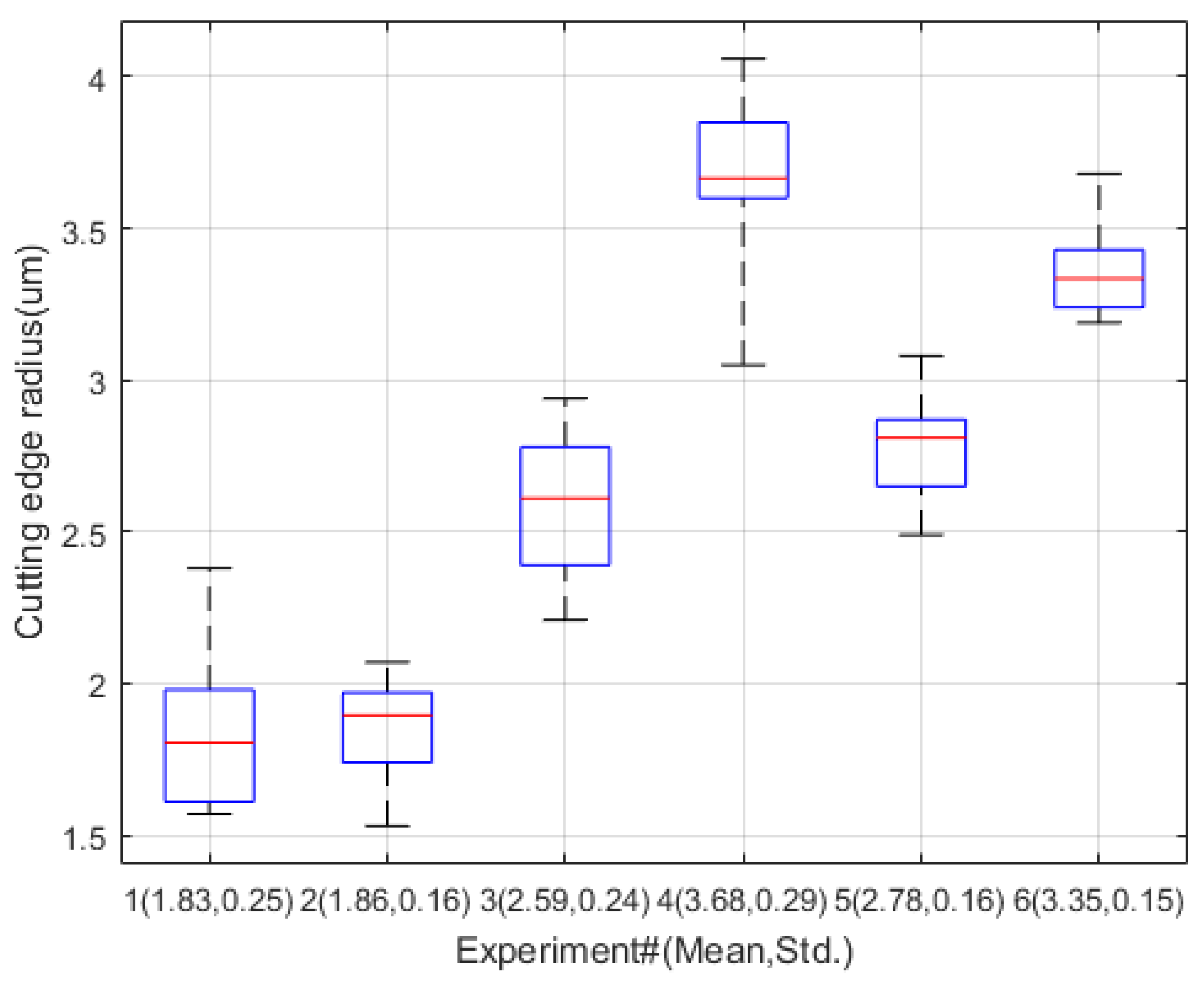
The cutting edge radius of the tool used in the previous experiment was measured by using a microscope (Olympus MX50) and by applying an image processing algorithm to calculate the corresponding MCT and the corresponding critical feedrate. The cutting edge radius measurements were then used in a simulation of chip production rate. Ten measurements were made from each cutting edge image from Exp. 1 to 6 and the means and the standard deviations are obtained as shown in Figure 1.
2.2. Previous Experiment
A schematic diagram of the experimental setup is shown in Figure 2. Six sets of cutting tests were performed with a 2-flute 200 μm endmill and brass workpiece [32]. The spindle speed and the depth of cut were set to 80,000 rpm and 40 μm, respectively. The purpose of the tests was to observe the drops between the number of chips obtained when the UCT is larger than the MCT and when the UCT is smaller than the MCT. Therefore, the feedrate was increased from 1 mm/s to 6 mm/s by 1 mm/s per slot and six slots were cut in each test set. The chips were sucked during the cutting process by using a material conveying pump and blown on an adhesive tape while the tape was being unwound by a pully attached to a motor shaft. Images of the chips were taken by a USB microscope. Thirty images of the tape with chips were obtained per slot. The number of chips was determined by applying image processing to the images.
The next section explains the process of finding the conditions under which the proposed cutting edge radius estimator will perform best.
3. Calibration
The cutting edge radius estimator can be considered as a kind of sensor that measures the cutting edge radius by detecting the chip number drop. The sensor needs to be calibrated whenever the operating conditions change. The purpose of the calibration for this sensor is to detect the drop in the number of chips more accurately. Previous studies have shown that a large drop in the number of chips can be seen in the number of chips above a certain size [32,33]. The calibration of this sensor is to find the appropriate threshold of size filtering to filter out chips smaller than a certain size and to count only the number of large chips.
In a chip production rate simulation, the volume of the chips is calculated. The unit for the size filtering threshold values for simulation is in . In the experiment, the chip size is obtained from the 2-D images. Therefore, the unit for the size filtering values for the experiment is in pixels. Since the values have different units, they are considered separately.
3.1. Size Filtering Threshold for Simulation Data
First, the size threshold for the simulation is found as follows: The simulation results of the chip number with three different cutting edge radii are shown in Figure 3. The chip production rate simulation requires a value for the number of tooth passes as an input parameter. The number of tooth passes for the simulation is determined based on the experimental set-up as follows: The size of the image is 1900 pixels by 1400 pixels, and the conversion factor from pixel to mm is 0.0048 mm/pixel. The length of the image of the tape which is 1900 pixels is used to calculate the time taken for the tape to travel a distance corresponding to 1900 pixels. The cutting time can be calculated from the tape speed and the size of the image. From this information, the number of tooth passes during the time is estimated as 1469.
Increasing the size filtering threshold reduces the number of chips as it filters more chips smaller than the threshold. The proper size filtering threshold should be a value within a range that allows for the detection of large drops in the number of chips at the critical feedrate. For example, in Figure 3a, if the critical feedrate is 1.6 mm/s, the number of chips drops sharply from feedrate 2 mm/s (above the critical feedrate) to 1 mm/s (below the critical feedrate) at the size filtering threshold of 5000. Similarly, in Figure 3b, if the critical feedrate is 2.4 mm/s, the number of chips has a large drop between feedrate 3 mm/s (above the critical feedrate) and 2 mm/s (below the critical feedrate) with the size filtering threshold of 5000. In Figure 3c, the number of chips also drops sharply between feedrate 4 mm/s and 3 mm/s at the size filtering threshold of 5000, if the critical feedrate is 3.2 mm/s. Therefore, the proper size filtering threshold for the simulation is determined to be 5000.
3.2. Size Filtering Threshold for Experimental Data
Next, the size filtering threshold for the experiments is determined. In this process, the simulation results and the experimental results are linearly fitted. Experimental chip number data is collected from a set of images of chips produced during a cutting process. Thirty images are taken in each feedrate as explained in Section 2.2. Therefore, 180 images are taken in each experiment.
From each set of 30 images, 20 images are randomly selected as the training data and the remaining 10 images are used as the testing data. The training data is used for the calibration process.
In order to find the experimental size filtering threshold that gives the maximum R-squared value, the filtering threshold is swept from 20 to 450. The maximum R-squared values are selected between the filtering thresholds of 20–250, since the number of chips becomes significantly small when the threshold becomes larger than 250 as shown in Figure 4. The optimum threshold is selected as listed in Table 1. The results from the linear fitting using the optimum thresholds are shown in Figure 5.
The reason why the filtering thresholds are different for each experiment is that the experimental conditions are changed in parts that are not controlled by the system. For example, when the system equipment is dismantled and then re-assembled, there can be variations in conditions such as the distance between the microscope and the tape, the precise focus position of the microscope, and so on. Therefore, in each experiment, this calibration process should be conducted.
3.3. Drop Detection Threshold
The key to the cutting edge radius estimation is to detect the drops in the number of chips when the MCT becomes larger than the UCT. After finding the first calibration parameter (size filtering threshold) of the estimator, the number of chips obtained from the experiment is applied as the input signal.
The output signal of the sensor can be obtained as shown in Equation (1).
Equation (1) is the sensor response curve for this estimator. The offset and slope values are obtained from the first calibration process.
In order to see the result after the first calibration, Equation (1) is applied to the testing data to get the output data from the calibrated estimator.
In this experiment, it is important to detect the drops in the number of chips as the feedrate crosses the critical feedrate. However, not only does the number of chips drop when the feedrate crosses the critical feedrate, but also the number of chips drops between the other feedrates as shown in Figure 6. Therefore, an additional process is needed to be able to distinguish the number drop at the critical feedrate from the other number drops at the other feedrates.
We begin by proposing that the drop in the number of chips at the critical feedrate is larger than the drops that occur at other feedrates. In order to distinguish the large drop from the other small drops, a drop detection threshold is introduced. This threshold represents the decrease in the chip number in percentage. For example, when the number of chips is reduced by 20% between feedrate 3 mm/s and 2 mm/s and the other drop is 30% between feedrate 2 mm/s and 1 mm/s, the feedrate range between the feedrate of 2 mm/s and 1 mm/s is selected with the threshold of 25% as the critical feedrate range that includes the actual critical feedrate.
The thresholds from 10–50% are applied to the training data to find a value that gives the highest probability of estimation as shown in Figure 7. The optimum threshold and the maximum probability values are listed in Table 2. A method of estimating the cutting edge radius and obtaining the probability of estimation is described in the next section.
4. Cutting Edge Radius Estimation
In order to evaluate the reliability of the cutting edge radius estimator, the probability of detecting the drop in the number of chips between the feedrates above and below the critical feedrate should be investigated.
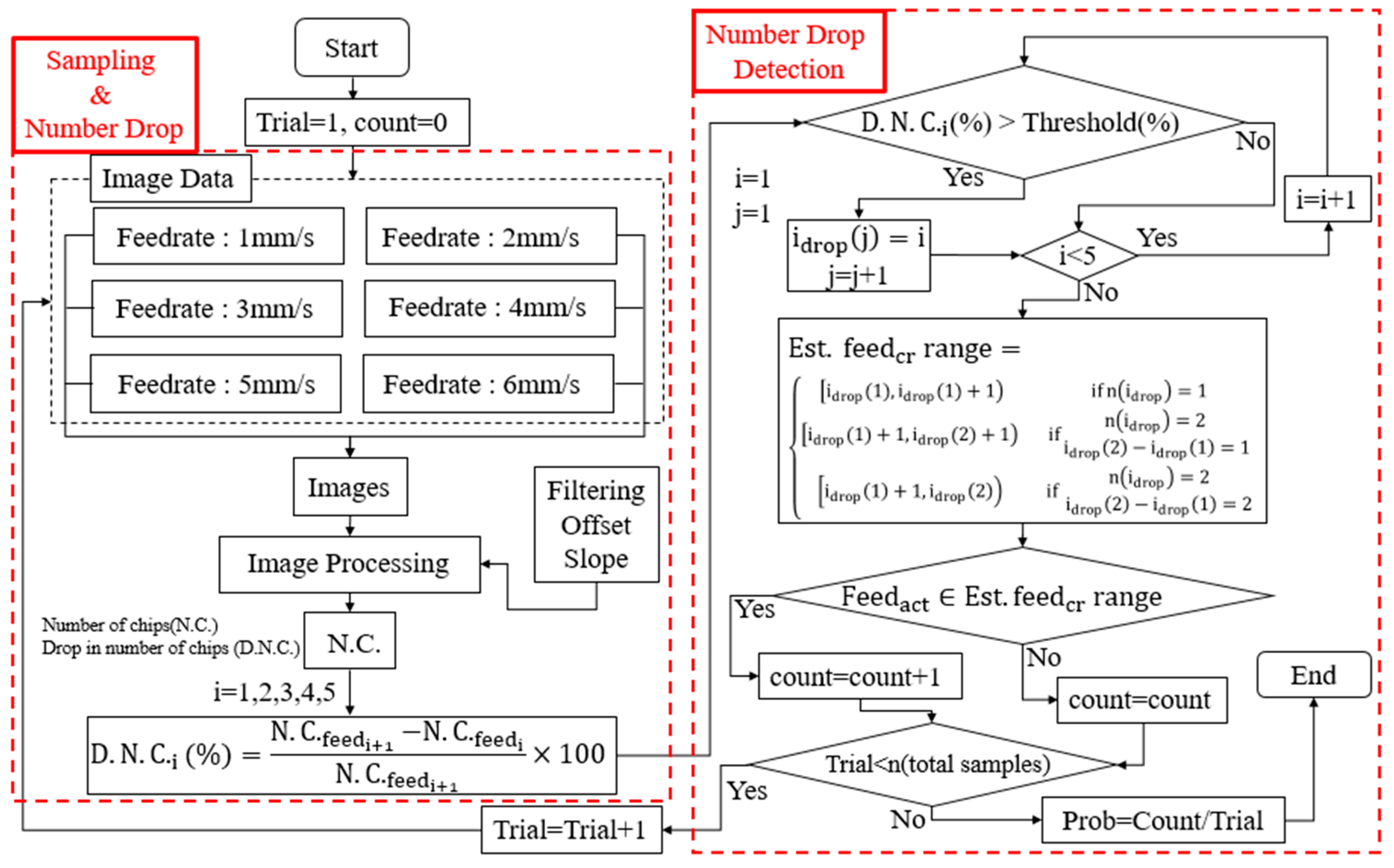
In Figure 8, a flow chart which explains how to calculate the probability of correctly estimating the cutting edge radius is presented. In this calculation, only the testing data is used. Ten images that are not used in the calibration are selected from each different feedrate as the testing data. The difference in the number of chips is calculated as follows: the difference between the number of chips at feedrate 6 mm/s and the number of chips at feedrate 5 mm/s is calculated. Then, the difference between the number of chips at feedrate 5 mm/s and the number of chips at feedrate 4 mm/s is calculated. In this order, the difference between the number of chips at feedrate 2 mm/s and the number of chips at feedrate 1 mm/s is calculated at the end. This process creates a new sample composed of the number differences that is used for the drop detection.
The total number of this new set of samples is since each data set from 6 different feedrates has 10 distinct numbers. Among those samples, if the number drop is detected at a certain feedrate range and the actual critical feedrate is in that range, then the estimation is successful. The probability of estimation can be obtained by dividing the number of successful estimation by the total number of samples.
5. Result
The cutting edge radius estimator is calibrated for each experiment, utilizing only the training data. The estimator is then applied to the testing data. The optimum size filtering threshold, the optimum drop detection threshold, the slope, and the offset values are used in the probability calculation.
The accuracy of the estimator is evaluated by calculating the probability of having the actual critical feedrate in the estimated critical feedrate range as listed in Table 3. The actual critical feedrates are obtained from the measured cutting edge radius. The number of samples is as described in Section 4. Only the feedrates from 1–4 mm/s are shown in the results since the actual critical feedrates are in the smaller range of 1–2 mm/s. When the number drop could not be detected, the probability of ‘none detected’ is also considered. And, the resolution of the estimation is limited to 1 mm/s due to the feedrate increment of 1 mm/s.
In Exp. 1, the actual critical feedrate is correctly estimated to within 1 mm/s with a probability of 76.95%. But, there are 10.05% of samples without any drop detection. In Exp. 2, the actual critical feedrate is between 1–2 mm/s, and this is correctly estimated 98.81% of the time. In Exp. 3, the actual critical federate of 2.07 mm/s is correctly estimated to be within 1 mm/s with a probability of 64.91%. The probability of estimating wrong ranges of 1–2 mm/s and 3–4 mm/s are 17.29% and 17.05%, respectively. The probability of estimating the actual critical feedrate within 1 mm/s in Exp. 4 is 74.29%. In Exps. 5 and 6, the probability of estimating the actual critical feedrate within 1 mm/s are 92.67% and 96.66%, respectively.
6. Conclusions
In this paper, the reliability of a new cutting edge radius estimator based on chip production rate for micro milling is evaluated. The size filtering threshold and the number difference threshold values can be regarded as calibration parameters, and a method of calibration is proposed and reported. A set of sample data is split into two sets: training data and testing data. The training data is used for the calibration, and the testing data is used for the evaluation. The optimum size filtering threshold values which generate the highest R-squared value from the linear curve fitting between the number of chips from the simulation and the experiment are determined in order to produce a sensor response curve for the estimator. Also, the optimum drop detection threshold values for the maximum probability of estimation is obtained as a part of the calibration process. The testing data is used for the evaluation of the reliability of the estimator.
The following conclusions have been drawn from the results.
- The average value of the probabilities of correct estimation from the experiments is 84.05%. The probabilities of correct estimation from the experiments are more than 70% except in Exp. 3 with 64.91%. Exps. 2, 5, and 6 show probabilities of correct estimation above 90%.
- In Exps. 1, 3, and 4, the standard deviation values of the actual critical feedrates are larger than the standard deviation values from the other experiments. As a result, the probabilities of wrong estimation are larger in Exps. 1, 3, and 4 than in Exps. 2, 5, and 6, due to the influence of the standard deviation on the estimation.
- The critical feedrate in this experiment can be only approximated to within 1mm/s. Since the feedrate increment in the experiment is 1 mm/s, it is only possible to estimate what feedrate range the critical feedrate is within. Further experiments are needed to determine if a higher precision of estimation is possible by using a feedrate increment smaller than 1 mm/s.
Development of an on-line cutting edge radius estimation system is planned as a future work [35]. If the drop in the number of chips could be detected during the cutting process, the cutting edge radius data may be able to be obtained automatically resulting in developing a cutting edge wear rate model.
Author Contributions
Conceptualization, A.A.S; methodology, J.-H.L and A.A.S; software, J.-H.L and A.A.S; validation, J.-H.L and A.A.S; investigation, J.-H.L and A.A.S; resources, A.A.S; writing—original draft preparation, J.-H.L; writing—review and editing, A.A.S; visualization, J.-H.L; supervision, A.A.S;
Funding
This research received no external funding.
Conflicts of Interest
The authors declare no conflict of interest.
References
- Alting, L.; Kimura, F.; Hansen, H.N.; Bissacco, G. Micro Engineering. CIRP Ann. 2003, 52, 635–657. [Google Scholar] [CrossRef]
- Masuzawa, T. State of the Art of Micromachining. CIRP Ann. 2000, 49, 473–488. [Google Scholar] [CrossRef]
- Dornfeld, D.; Min, S.; Takeuchi, Y. Recent advances in mechanical micromachining. CIRP Ann. 2006, 55, 745–768. [Google Scholar] [CrossRef]
- Kussul, E.M.; Rachkovskij, D.A.; Baidyk, T.N.; Talayev, S.A. Micromechanical engineering: A basis for the low-cost manufacturing of mechanical microdevices using microequipment. J. Micromech. Microeng. 1996, 6, 410. [Google Scholar] [CrossRef]
- Kim, C.-J.; Mayor, J.R.; Ni, J. A Static Model of Chip Formation in Microscale Milling. J. Manuf. Sci. Eng. 2005, 126, 710–718. [Google Scholar] [CrossRef]
- Sodemann, A.; Li, M.; Mayor, R.; Forest, C.R. Micromilling of molds for microfluidic blood diagnostic devices. In Proceedings of the 24th Annual Meeting of the American Society for Precision Engineering, Monterey, CA, USA, 4–9 October 2009; pp. 4–9. [Google Scholar]
- Guckenberger, D.J.; de Groot, T.E.; Wan, A.M.D.; Beebe, D.J.; Young, E.W.K. Micromilling: A method for ultra-rapid prototyping of plastic microfluidic devices. Lab Chip 2015, 15, 2364–2378. [Google Scholar] [CrossRef] [PubMed] [Green Version]
- Owens, C.E.; Hart, A.J. High-precision modular microfluidics by micromilling of interlocking injection-molded blocks. Lab Chip 2018, 18, 890–901. [Google Scholar] [CrossRef] [PubMed]
- Aramcharoen, A.; Mativenga, P.T. Size effect and tool geometry in micromilling of tool steel. Precis. Eng. 2009, 33, 402–407. [Google Scholar] [CrossRef]
- Zhanqiang, L.; Zhenyu, S.; Yi, W. Definition and determination of the minimum uncut chip thickness of microcutting. Int. J. Adv. Manuf. Technol. 2013, 69, 1219–1232. [Google Scholar] [CrossRef]
- Liu, X.; DeVor, R.E.; Kapoor, S.G. An analytical model for the prediction of minimum chip thickness in micromachining. J. Manuf. Sci. Eng. 2006, 128, 474–481. [Google Scholar] [CrossRef]
- Ziegert, J.C.; Pathak, J.P.; Jokiel, B. An Ultra-high Speed Spindle for Micro-milling. In Proceedings of the ASPE, Portland, OR, USA, 26–31 October 2003. [Google Scholar]
- Lu, X.; Wang, F.; Jia, Z.; Liang, S.Y. The flank wear prediction in micro-milling Inconel 718. Ind. Lubr. Tribol. 2018, 70, 1374–1380. [Google Scholar] [CrossRef]
- Mayor, J.R.; Sodemann, A.A. Intelligent tool-path segmentation for improved stability and reduced machining time in micromilling. J. Manuf. Sci. Eng. 2008, 130, 031121. [Google Scholar] [CrossRef]
- Przestacki, D.; Chwalczuk, T.; Wojciechowski, S. The study on minimum uncut chip thickness and cutting forces during laser-assisted turning of WC/NiCr clad layers. Int. J. Adv. Manuf. Technol. 2017, 91, 3887–3898. [Google Scholar] [CrossRef] [Green Version]
- Ducobu, F.; Filippi, E.; Rivière-Lorphèvre, E. Chip formation and minimum chip thickness in micro-milling. In Proceedings of the 12th CIRP Conference on Modeling of Machining Operations, Donostia-San Sebastian, Spain, 7–8 May 2009; pp. 339–346. [Google Scholar]
- Oliaei, S.N.B.; Karpat, Y. Influence of tool wear on machining forces and tool deflections during micro milling. Int. J. Adv. Manuf. Technol. 2016, 84, 1963–1980. [Google Scholar] [CrossRef]
- Filiz, S.; Conley, C.M.; Wasserman, M.B.; Ozdoganlar, O.B. An experimental investigation of micro-machinability of copper 101 using tungsten carbide micro-endmills. Int. J. Mach. Tools Manuf. 2007, 47, 1088–1100. [Google Scholar] [CrossRef]
- Uriarte, L.; Azcárate, S.; Herrero, A.; Lopez de Lacalle, L.N.; Lamikiz, A. Mechanistic modelling of the micro end milling operation. Proc. Inst. Mech. Eng. Part B J. Eng. Manuf. 2008, 222, 23–33. [Google Scholar] [CrossRef]
- Alhadeff, L.L.; Marshall, M.B.; Curtis, D.T.; Slatter, T. Protocol for tool wear measurement in micro-milling. Wear 2019, 420–421, 54–67. [Google Scholar] [CrossRef]
- Ng, C.K.; Melkote, S.N.; Rahman, M.; Kumar, A.S. Experimental study of micro- and nano-scale cutting of aluminum 7075-T6. Int. J. Mach. Tools Manuf. 2006, 46, 929–936. [Google Scholar] [CrossRef]
- Weule, H.; Hüntrup, V.; Tritschler, H. Micro-Cutting of Steel to Meet New Requirements in Miniaturization. CIRP Ann. 2001, 50, 61–64. [Google Scholar] [CrossRef]
- Bissacco, G.; Hansen, H.N.; De Chiffre, L. Size Effects on Surface Generation in Micro Milling of Hardened Tool Steel. CIRP Ann. 2006, 55, 593–596. [Google Scholar] [CrossRef] [Green Version]
- Rehorn, A.G.; Jiang, J.; Orban, P.E.; Bordatchev, E.V. State-of-the-art methods and results in tool condition monitoring: A review. Int. J. Adv. Manuf. Technol. 2004, 26, 942. [Google Scholar] [CrossRef]
- Thepsonthi, T.; Özel, T. Experimental and finite element simulation based investigations on micro-milling Ti-6Al-4V titanium alloy: Effects of cBN coating on tool wear. J. Mater. Process. Technol. 2013, 213, 532–542. [Google Scholar] [CrossRef]
- Ucun, İ.; Aslantas, K.; Bedir, F. An experimental investigation of the effect of coating material on tool wear in micro milling of Inconel 718 super alloy. Wear 2013, 300, 8–19. [Google Scholar] [CrossRef]
- Zhou, L.; Peng, F.Y.; Yan, R.; Yao, P.F.; Yang, C.C.; Li, B. Analytical modeling and experimental validation of micro end-milling cutting forces considering edge radius and material strengthening effects. Int. J. Mach. Tools Manuf. 2015, 97, 29–41. [Google Scholar] [CrossRef]
- Tansel, I.N.; Bao, W.Y.; Reen, N.S.; Kropas-Hughes, C.V. Genetic tool monitor (GTM) for micro-end-milling operations. Int. J. Mach. Tools Manuf. 2005, 45, 293–299. [Google Scholar] [CrossRef]
- Hsieh, W.-H.; Lu, M.-C.; Chiou, S.-J. Application of backpropagation neural network for spindle vibration-based tool wear monitoring in micro-milling. Int. J. Adv. Manuf. Technol. 2012, 61, 53–61. [Google Scholar] [CrossRef]
- Ren, Q.; Balazinski, M.; Baron, L.; Jemielniak, K.; Botez, R.; Achiche, S. Type-2 fuzzy tool condition monitoring system based on acoustic emission in micromilling. Inf. Sci. 2014, 255, 121–134. [Google Scholar] [CrossRef]
- Zhu, K.; Mei, T.; Ye, D. Online Condition Monitoring in Micromilling: A Force Waveform Shape Analysis Approach. IEEE Trans. Ind. Electron. 2015, 62, 3806–3813. [Google Scholar]
- Lee, J.-H.; Sodemann, A.A.; Bajaj, A.K. Experimental Validation of Chip Production Rate as a Tool Wear Identification in Micro-EndMilling. Int. J. Adv. Manuf. Technol. (accepted).
- Lee, J.-H.; Sodemann, A.A. Geometrical Simulation of Chip Production Rate in Micro-EndMilling. Procedia Manuf. 2018, 26, 209–216. [Google Scholar] [CrossRef]
- Lee, J.-H.; Sodemann, A.A. Digital Image Processing for Counting Chips in Micro-End-Milling. In Proceedings of the 2nd International Conference on Vision, Image and Signal Processing, Las Vegas, NV, USA, 27–29 August 2018; p. 9. [Google Scholar]
- Lee, J.-H.; Sodemann, A.A. Simulation of Cutting Edge Wear Model based on Chip Production Rate in Micro-endmilling. In Proceedings of the ASME 2019 14th International Manufacturing Science and Engineering Conference (MSEC2019), Erie, PA, USA, 10–14 June 2019. [Google Scholar]
Figure 1.
Box plot of cutting edge radius with mean and standard deviation.

Figure 2.
A schematic diagram of experimental setup [34].
Figure 2.
A schematic diagram of experimental setup [34].

Figure 3.
Size filtering and number of chips from the simulation with the cutting edge radius (critical feedrate) of (a) 2 (1.6 mm/s), (b) 3 (2.4 mm/s), and (c) 4 (3.2 mm/s).
Figure 3.
Size filtering and number of chips from the simulation with the cutting edge radius (critical feedrate) of (a) 2 (1.6 mm/s), (b) 3 (2.4 mm/s), and (c) 4 (3.2 mm/s).

Figure 4.
Relationship between the experimental filtering threshold and R-squared values from the linear fitting from (a) Exp. 1 to (f) Exp. 6.
Figure 4.
Relationship between the experimental filtering threshold and R-squared values from the linear fitting from (a) Exp. 1 to (f) Exp. 6.

Figure 5.
Linear fit of the number of chips from the simulation and the experiment with the optimum experimental size filtering threshold from (a) Exp. 1 to (f) Exp. 6.
Figure 5.
Linear fit of the number of chips from the simulation and the experiment with the optimum experimental size filtering threshold from (a) Exp. 1 to (f) Exp. 6.

Figure 6.
Normal distribution of the output signal and the critical feedrate boundary (Mean, Std.) from (a) Exp. 1 (1.46 mm/s, 0.196 mm/s), (b) Exp. 2 (1.49 mm/s, 0.127 mm/s), (c) Exp. 3 (2.07 mm/s, 0.188 mm/s), (d) Exp. 4 (2.94 mm/s, 0.23 mm/s), (e) Exp. 5 (2.23 mm/s, 0.132 mm/s), and (f) Exp. 6 (2.68 mm/s, 0.12 mm/s).

Figure 7.
Drop detection threshold and probability of estimation from (a) Exp. 1 to (f) Exp. 6.

Figure 8.
A flow chart of calculating the probability of estimation.


Table 1.
Optimum experimental size filtering threshold with maximum R-squared value.
| Exp. | Experimental Size Filtering Threshold | |||
|---|---|---|---|---|
| Optimum Filtering Threshold | Maximum r-Squared | Slope | Y-Intercept (Offset) | |
| 1 | 47 | 0.83 | 0.14 | 63.76 |
| 2 | 126 | 0.80 | 0.24 | –132.23 |
| 3 | 124 | 0.88 | 0.15 | 10.46 |
| 4 | 150 | 0.85 | 0.13 | 9.46 |
| 5 | 172 | 0.94 | 0.14 | –14.48 |
| 6 | 116 | 0.91 | 0.23 | –36.81 |
Table 2.
Optimum drop detection threshold and maximum probability of estimation.
| Exp. | Probability of Estimation and Threshold (%) | |
|---|---|---|
| Optimum Threshold (%) | Max. Probability (%) | |
| 1 | 27 | 78 |
| 2 | 23 | 99 |
| 3 | 25 | 62 |
| 4 | 31 | 77 |
| 5 | 25 | 92 |
| 6 | 25 | 97 |
Table 3.
Probability of critical feedrate estimation from (a) Exp.1 to (f) Exp.6.
| Exp. | Actual Critical Feedrate (mm/s) (Mean (±Std.)) | Probability of Estimation (%) | ||||
|---|---|---|---|---|---|---|
| Estimated Critical Feedrate | ||||||
| 1–2 mm/s | 2–3 mm/s | 3–4 mm/s | 4–5 mm/s | None | ||
| 1 | ) | 76.95 | 13.00 | 0.00 | 0.00 | 10.05 |
| 2 | 98.81 | 0.49 | 0.01 | 0.00 | 0.69 | |
| 3 | 17.29 | 64.91 | 17.05 | 0.75 | 0.75 | |
| 4 | 7.27 | 74.29 | 18.44 | 0.00 | 0.00 | |
| 5 | 4.92 | 92.67 | 0.32 | 2.10 | 2.10 | |
| 6 | 2.01 | 96.66 | 1.22 | 0.00 | 0.11 | |
© 2019 by the authors. Licensee MDPI, Basel, Switzerland. This article is an open access article distributed under the terms and conditions of the Creative Commons Attribution (CC BY) license (http://creativecommons.org/licenses/by/4.0/).
Share and Cite
MDPI and ACS Style
Lee, J.-H.; Sodemann, A.A. Reliability of Cutting Edge Radius Estimator Based on Chip Production Rate for Micro End Milling. J. Manuf. Mater. Process. 2019, 3, 25. https://doi.org/10.3390/jmmp3010025
AMA Style
Lee J-H, Sodemann AA. Reliability of Cutting Edge Radius Estimator Based on Chip Production Rate for Micro End Milling. Journal of Manufacturing and Materials Processing. 2019; 3(1):25. https://doi.org/10.3390/jmmp3010025
Chicago/Turabian StyleLee, Jue-Hyun, and Angela A. Sodemann. 2019. "Reliability of Cutting Edge Radius Estimator Based on Chip Production Rate for Micro End Milling" Journal of Manufacturing and Materials Processing 3, no. 1: 25. https://doi.org/10.3390/jmmp3010025