
Forces Shapes in 3-Axis End-Milling: Classification and Characteristic Equations


Department of Industrial Engineering, University of Firenze, via di Santa Marta 3, 50139 Firenze, Italy
*
Author to whom correspondence should be addressed.
J. Manuf. Mater. Process. 2021, 5(4), 117; https://doi.org/10.3390/jmmp5040117
Submission received: 20 September 2021
/
Revised: 26 October 2021
/
Accepted: 28 October 2021
/
Published: 29 October 2021
Abstract
:In 3-axis milling, cutting force analysis represents one of the main methods to increase the quality and productivity of the process. In this context, cutting force shape gives information of both monitoring and prediction of the cutting process. However, the cutting force shape is not unique, and it changes according to the cutting strategy, tool geometry, and cutting parameters. This paper presents a comprehensive approach to predict and classify cutting force shapes in 3-axis milling operations. In detail, the proposed approach starts by classifying the cutting force shapes for a single fluted endmill (i.e., single flute force shape), and, considering how the single flute force shapes may overlap one another, it extends the classification to a general multiple-fluted endmill. Moreover, the method provides, through analytical equations, angles, and magnitude dimensionless parameters of each key point, describing each shape classified. Finally, the proposed approach was experimentally validated through several milling tests in different cutting conditions.
1. Introduction
The milling process is, by far, the most flexible and common machining process in modern manufacturing. The ever-increasing need for high accuracy and productivity has led to the development of advanced monitoring and predictive approaches [1]. The interaction forces between tool and workpiece, known as cutting forces, are an essential input for several of these approaches since they can reveal the effects of different key aspects of the process, such as tool wear [2], engagement conditions [3], vibrations [4], surface error [5,6]. In milling such cutting forces are not constant during the process and their shape and magnitude change significantly with cutting process parameters [7]. Different cutting force models have been proposed in the literature, and most of them relate cutting forces to the chip thickness by utilizing cutting force coefficients [8,9,10]. In peripheral milling, chip thickness can be fairly approximated by sinusoidal functions, however, this simple formulation is valid for straight teeth tools (i.e., zero helix angle) which are practically never adopted in actual operations [11]. Therefore, the approximated cutting forces, computed by such models, are not suitable for force shape prediction, yet they can be only applied to predict surface errors (e.g., surface location error [12]), or vibrations phenomena (e.g., chatter [13,14]), showing several limitations.
Indeed, the tool helix angle changes significantly the cutting force shape since it affects both exit and entry angles, chip area, and it has a direct effect on the surface error variation along with the axial depth of cut [15]. To obtain a reliable and accurate cutting force prediction, including the tool helix angle, chip thickness sinusoidal approximation must be applied to small discs in which the tool should be divided along its axis, leading to cutting force prediction through numerical methods [16,17,18].
However, quick analytical information about the expected cutting forces could be very useful in monitoring solutions (e.g., depth of cut identification [19], feed adjustment [20]). Indeed, measured cutting forces can return high-value information regarding the actual process, and, along with the expected cutting forces, they allow the process to be controlled by adjusting the cutting parameters [21]. Analytical information on cutting forces can be obtained using a frequency domain solution [22,23], but the proposed equations are valid only for a specific cutting force model and require cutting force coefficients [24]. On the other hand, accurate identification of cutting force shape could allow the cutting force to be predicted only at specific instants, dramatically reducing the computational efforts of predictive approaches. Hence, it is clear that an analytical representation of cutting force shape including the effects of cutting parameters could be effectively exploited, even without cutting force magnitude prediction [25,26]. In the last decades, several works have tried to define and classify the cutting force shapes in peripheral milling providing simple equations to represent them.
The work of Choi et al. [27] was one of the first investigations on the relation between force shape and flutes engagements, and the authors developed a method to predict depts of cut in end-milling exploiting this information. Yun et al. [15] computed the position of the peak value of the cutting force through analytical equations. Although effective, their approaches apply only to specific conditions. Yang et al. [28] identified different force shapes with dedicated equations, to detect the depth of cut variations. Their results prove that force shapes are not unique, but, even in this case, only down-milling operations and certain conditions are investigated. Islam et al. [29] and Desai et al. [30] started from these classifications to predict surface error shapes. All the results presented do not give a comprehensive picture of all the force shapes. Indeed, the authors focused their attention only on specific cases: down milling operations with two flutes cutting simultaneously in defined cutting conditions. Moreover, analytical equations for force shape serve to predict characteristic angles without considering the cutting force magnitude variation.
In this work, a comprehensive classification of cutting force shapes is proposed, and specific formulations are presented, considering cutting parameters combinations and different configurations (i.e., up and down milling). Cutting force shapes are classified, and for each type of characteristic equations, which identify the key angles are presented, extending the ones presented by Yang et al. [28]. In addition, magnitude variation was investigated, assigning to each key point, a binary value (i.e., 0 or 1), that allows a simplified representation of the normalized total cutting force shape. The proposed formulations were experimentally validated through cutting tests in several conditions, showing the different force shapes, as classified by the proposed approach.
The proposed classification and formulations return the expected shape of the cutting force without the need for any simulation or cutting force model. For this reason, they could be used to efficiently predict cutting force only on specific points. Moreover, the proposed approach could lay the ground for monitoring solutions based on cutting force signals.
2. Materials and Methods
Cutting force shape is not unique, but it changes according to the tool geometry (tool diameter D, helix angle αel, number of flutes N), the cutting parameters (radial depth of cut ar, axial depth of cut ap), and the cutting strategy (down-milling or up-milling).
In this work, all the shapes which the total cutting force F (i.e., resultant of cutting force in the x-y plane, as shown in Figure 1) could assume are analyzed and a comprehensive classification is provided, starting from a single fluted endmill (N = 1) to a generical multiple-fluted endmill (N > 1), as partially presented in [7,28].
Each shape is identified by key points, whose coordinates are expressed through the angular position (i.e., key angle) and a binary value (m) which is related to the magnitude of the cutting and defined in this work as:
m = 1 when cutting force is maximum
m = 0 when cutting force is minimum
m = 0 when cutting force is minimum
These formulations are valid in one period, wide as the tool pitch angle (ϕz), which marks the periodicity of the cutting force (neglecting tool run-out). Tool pitch angle, assuming equally spaced flutes for the endmill, can be defined as:
2.1. Shape Classification in Single-Fluted Endmill
The proposed classification starts with the definition of the different types of F shape for a single fluted endmill (N = 1). In this condition, key points’ coordinates (i.e., key angles-m values couples) are based on a set of working angles that can be obtained directly from the cutting parameters (ar, ap) and the tool geometry (D, αel).
2.1.1. Key Angles
The proposed formulations start from the basic angles already presented by other authors [7,28]. The axial engagement angle αsw is related to ap and the endmill’s geometry following the equations:
where αel is the tool helix angle and D is the tool diameter.
The radial engagement angle αen is defined using radial depth of cut ar with the following equation:
Moreover, a critical value for both αen and αsw is necessary for the classification. The critical axial engagement angle αswc is the axial engagement angle that equals αen Equation (6) [28].
The critical radial engagement angle αenc is defined as the engagement angle which identifies the angular position of the maximum of F in a slotting condition. It must be noted that, due to the different kinematic of the cut, αenc changes from down-milling to up-milling, however, in both cases, it is related to the maximum chip thickness [28].
These working angles, already presented in other works, are used to express the key angles, which identify the angular position of the key points of the F shape for a single fluted endmill, with the following proposed equations:
Each key angle represents a specific angular position of the cutting process. In detail, the cut starts when the cutting edge reaches ϕin, and it ends when the same cutting edge reaches ϕout (Figure 2). However, due to the helix angle, the cutting edge reaches these positions at the bottom of ap and the top of ap. Therefore, ϑ1 represents the angular positions of the cutting edge when it starts cutting at the bottom of ap, while ϑ3 is the angular position of the cutting edge when it starts cutting at the top of ap.
Following a similar concept, ϑ2 and ϑ4 are the angular positions of the cutting edge when it stops cutting at the bottom of the ap and the top of the ap.
On the other hand, ϑM, does not represent a particular position of the cutting edge, but it represents the angular position of the maximum value of F. Moreover, ϑM is relevant only in those operations where the ar exceeds the tool radius. It is interesting to note that all the key angles are only dependent on the tool’s geometry (αel, D) and the cutting parameters (ar, ap), without the need for any cutting force model or coefficients.
2.1.2. Magnitude Value
The m value, as defined in Equation (1), corresponding to the key angles ϑ1 and ϑ4 is 0, while for ϑ2, ϑ3, and ϑM the corresponding m value is 1. Indeed, ϑ1 and ϑ4 represent the beginning and the ending of the cutting process, therefore they identify a minimum of F. Instead ϑ2, ϑ3 and ϑM represent angular positions where the cutting edge is fully involved in the cut, thus they identify a maximum of F. However, the key points identified by ϑ2, ϑ3, and ϑM do not always contribute to the F shape because the angular position corresponds to F maximum changes according to both the cutting parameters (ar, ap) and the cutting strategy (down-milling or up-milling).
2.1.3. Classification
To comprehensively investigate the F shape for a single fluted endmill, the effects of the cutting parameters were studied, exploiting αsw and αen and their critical values (αenc and αswc) in both down-milling and up-milling. This analysis allows distinguishing three different F shapes, each one defined by a different set of key points. The characteristics of each F shape, referred to as Type, are described as follows:
- Type I: This shape occurs when conservative cutting parameters are adopted, and it presents αen greater than αsw. In down-milling, this type is identified by three key points (ϑ1, 0), (ϑ3, 1), and (ϑ4, 0). The type I shape reproduces a scalene triangle where the upper vertex, which represents the F maximum, is identified by ϑ3 because it is the angular position where the cutting edge is fully involved in the cut and the chip thickness is maximum. In up-milling, this type presents a scalene triangle shape defined by three key points (ϑ1, 0), (ϑ2, 1), and (ϑ4, 0). However, in this case, the F maximum is identified by ϑ2 because this key angle, in up-milling, represents the condition of cutting edge fully engaged and maximum chip thickness.
- Type II: This shape occurs when aggressive axial depths of cut are used, and it is characterized by αsw greater than αen. In both down-milling and up-milling, this type presents an isosceles trapezoid shape defined by four key points (ϑ1, 0), (ϑ2, 1), (ϑ3, 1) and (ϑ4, 0). In this case, the F maximum is identified by two different key angles because with high axial depths of cut the condition of cutting edge fully engaged and maximum chip thickness starts at ϑ2 and continues up to ϑ3. For this type, two subtypes are defined, IIa and IIb. The difference between type IIa and type IIb is related to the length of the upper base, which is less than half of the lower base length for type IIa and more than half of the lower base length for type IIb.
- Type III: This shape occurs when aggressive radial depths of cut are used, and it features αen greater than αenc. In down-milling, this type presents an acute trapezoid shape defined by four key points (ϑ1, 0), (ϑ3, 1), (ϑM, 1) and (ϑ4, 0). The F maximum is identified by ϑ3 and ϑM, but an important observation must be made. Indeed, ϑ3 is the angular position where the cutting edge is fully engaged, while ϑM is the angular position where the cutting edge is fully engaged, and the chip thickness is maximum. Therefore, the effective value of F at ϑ3 is smaller than the one at ϑM. Moreover, the magnitude value of F at ϑ3 cannot be known without simulating the cutting force. For this reason, even if F is not effectively maximum at ϑ3, the m value at ϑ3 is assumed to be 1. This simplification allows a fairly accurate representation of the type III F shape, without any simulation of the cutting forces. In up-milling type III also presents an acute trapezoid shape identified by four key points (ϑ1, 0), (ϑM, 1), (ϑ2, 1) and (ϑ4, 0). The same observation made for ϑ3 and ϑM in down-milling applies to ϑ2 and ϑM in up-milling.
The force profile types are shown in Table 1 with their occurrence conditions, a comparison between normalized cutting forces and the representation of the key points is shown in Figure 3. In detail, normalized cutting forces were obtained through numerical simulations using the cutting force model presented in [30] using 2000 points discretization for tool rotation and 1500 points discretization in the tool axis direction. Instead, key points for one period (from ϑ1 to ϑ1 + ϕz in down-milling and from ϑ4 − ϕz to ϑ4 in up-milling) are provided in Table 2. It must be pointed out that a cutting operation characterized by αen > αenc and αsw > αswc cannot occur, as it is easily verifiable by comparing αenc Equations (13) and (14) and αswc Equation (6). The types described are suitable for any 3-axis milling operation in which only one flute is involved in the cut. Nonetheless, milling operations are usually characterized by a concurrent cutting of several flutes, therefore this classification must be extended to a multiple-fluted endmill (N > 1).
2.2. Shape Classification in Multiple-Fluted Endmill
In the previous section, all the F shapes for a single fluted endmill were distinguished in types. These types are now used to characterize the F shape for a general multiple-fluted endmill (N > 1). Indeed, the F shape for a multiple-fluted endmill can be conceived as the sum of multiple single flute F types as it is shown in Figure 4 for a four-fluted endmill. Hence, the multiple flute F shape can be characterized by analyzing how single flute F shapes of the same type may overlap. Considering the geometric aspects of each type, the amount of overlap between the generic i single flute F shape and the following i + 1 single flute F shape was classified into six different degrees, as it is shown in Figure 5. In detail, the degrees of overlap defined are:
- No Overlap: This configuration applies to every type of single flute F shape, and it occurs when the generic i single flute F shape and the following i + 1 single flute F shape are not intersecting at all.
- Low Overlap (L): The low overlap condition involved all the types of single flute F shape. In detail, the low overlap takes place when the falling edge of the generic i single flute F shape affects the rising edge of the i + 1 single flute F shape.
- Medium Overlap (M): This overlap configuration is possible for every type as well. However, in this condition, the falling edge of the generic i single flute F shape alters two edges, rising and falling edge (type I, type III) or rising and constant portion (type IIa, type IIb), of the i + 1 single flute F shape.
- High Overlap (H): In the high overlap configuration the rising edge of the generic i single flute F shape affects the rising edge of the i + 1 single flute F shape. This case does not apply to type IIb.
- Deep medium overlap (m): The deep medium overlap verifies only for type IIb. In this condition the falling edge of the generic i single flute F shape influences the constant portion of the i + 1 single flute F shape, and, at the same time, the constant portion of the generic i single flute F shape influences the constant portion of the i + 1 single flute F shape.
- Deep high overlap (h): The deep high overlap applies to both type IIb and type IIa. In detail, this overlap occurs when the rising edge of the generic i single flute F shape affects the rising edge of the i + 1 single flute F shape, and, at the same time, the constant portion of the generic i single flute F shape alters the constant portion of the i + 1 single flute F shape.
In addition to type and overlap degree, the number of flutes involved in the cut (n) may significantly impact the multiple flutes F shape, especially in medium and high overlap configurations. Indeed, when n single flute F shapes are overlapping, it is crucial to define which key point of which single flute F shape is relevant for the resultant multiple flute F shape. Therefore, not only n but also the number of flutes involved in the axial engagement (called here v) becomes important to identify the key points for multiple flutes F shapes. For this reason, starting from the key angles for a single fluted endmill, a set of additional key angles for multiple flute F shapes are expressed for both down-milling and up-milling:
The m values corresponding to each additional key angle are defined according to the single flute F shape classification, so 0 is assigned when x is equal to 1 and 4, and 1 when x is equal to 2, 3, and M. The critical aspect for the key point representation of multiple flutes F shapes is related to the cutting parameters (ar, ap). Indeed, both the radial and axial depth of cut directly affect the slope of the edges of the single flute F shapes and, based on a number of flutes involved (n and v), some of the key points which may identify the F maximum for a single flute F shape, becomes irrelevant for the resultant multiple flutes F shapes. Therefore, to identify which key point is necessary to represent the multiple flutes F shape for a specific type/degree of overlap couple, a set of equations are proposed (18)–(23). These equations represent the conditions that must be fulfilled to make a key point relevant for the multiple flutes F shape.
The Equations (18) and (19) are valid for both down-milling and up-milling, while the others apply to either down-milling (20) or up-milling (21). Considering the cutting conditions and the type/degree of overlap combination, the key points representing the multiple flutes F shape in one period (from ϑ1 to ϑ1 + ϕz in down-milling and from ϑ4 − ϕz to ϑ4 in up-milling) are presented in Table 3 (down-milling) and Table 4 (up-milling). In both strategies, for type I and III, the multiple flutes F shape is easily identified by the proposed key points in any configurations, while for the other types (IIa, IIb) the proposed cutting conditions should be considered for the representation of the key points, for medium and deep medium overlap configurations. Furthermore, it is interesting to note that increasing the overlap degree, either by a reduced periodicity (i.e. increasing the number of flutes) or an increase of engagement conditions (i.e., ap and ar), the number of key points required to define the force shape is reduced. The proposed formulations are valid in peripheral milling, in the case of slotting (i.e., full immersion) overlaps may introduce different key points on the profile, caused by the change in the curvature of rising and falling edges.
3. Results and Discussion
3.1. Experimental Set-Up
Several milling tests were carried out to experimentally validate the proposed formulations and present the different force shapes. The tests were performed on a DMU 75 MONOBLOCK machine tool, provided by DMG MORI (Japan), on a stiff workpiece (50 × 80 × 90 mm) made of aluminum (6082-T4), clamped to a table dynamometer from Kitsler (Switzerland), model: 9257A to measure forces during the tests (Figure 6a). The dynamometer’s main characteristics are: ±5000 N of measuring range, 0.1 N resolution, 2.5 kHz resonance frequency (not considering machine-workpiece dynamics). Additional data are provided in the work of Scippa et al. where such device is used [31]. The different tool and cutting parameters combinations are presented in Table 5 and Table 6. These parameters have been designed to test the different categories classified in this work, both in terms of types and overlap degree. In particular:
- Two endmills were used to test different combinations of diameter and number of flutes: a four-fluted 12 mm tool (manufactured by Garant, Germany, model:202552, Figure 6b) and a three-fluted 10 mm tool (manufactured by Garant, Germany, model:202274, Figure 6c). Moreover, the two endmills allow testing of the same type and overlap configuration with different tool characters, as shown in this work for I type.
- The tools are characterized by the same helix angle equal to 45°, this value was selected since it is typical for the tested material (aluminum) and allows to achieve higher overlap degree with less aggressive parameters.
- Spindle speed and feed were selected for each tool according to the parameters suggested by the tool manufacturer and they were not changed in the different tests, since they did not affect the force shape, focus of the work.
- Depths of cut (ap and ar) were designed in order to perform the different types and overlap degrees, as found by the proposed approach. Indeed, as highlighted in the previous sections, it is not important the single value of ap or ar but the combination of both. Therefore, the couple of the depths of cut values were selected together to achieve the different configurations proposed in this work.
- The tests were repeated for Down-milling and Up-milling with slightly different parameters in order to return the same Type and Overlap configuration.
- The high and deep-high overlap configurations were not tested. These conditions required several flutes and aggressive cutting parameters (especially high ar), rarely employed in actual peripheral milling operations. Moreover, the high and deep-high overlap configurations often entail a simple triangle-shaped cutting force profile, less interesting to be investigated.
- Lastly, tests 33 and 34 were performed to highlight some differences between the similar tests, as presented in the discussion section.
Tool proprieties, spindle speed, and feed per tooth used are summarized in Table 5 for both tools. In Table 6 the different tests are reported, including engagement conditions and the combination type and overlap of the specific test. As highlighted in the table, almost all the classified configurations were tested, except for high and deep-high overlap.
For each test, the cutting forces were measured in the three normal directions (X, Y, Z) using the dynamometer. The measured forces were then compensated to reduce the distortion derived by the system dynamics [32,33] using the approach proposed by Scippa et al. [31], and post-processed to reduce measurement noise. As well as this, the impact of tool run-out was compensated as in [8].
Since the focus of the proposed method is the total force (i.e., resultant of the tangential and radial forces), the next step was the computation of such force by combining X-force (feed direction) and Y-force (cross-feed direction).
The measured forces were then normalized to assume values between 0 and 1, obtaining the unity based normalized total forces, called F* which is summarized by the following equation:
where Fk is the generic k value of F in one period, while max (F) and min (F) represent the maximum and minimum values of F in one period.
The computed normalized total forces were grouped based on the type and shown in the next figures (Figure 6, Figure 7, Figure 8, Figure 9 and Figure 10). The different F* were shown in the engagement angle range corresponding to one period, which is equal from ϑ1 to ϑ1 + ϕz in down-milling and from ϑ4 − ϕz to ϑ4 in up-milling. To improve the readability of the figures, even engagement angle has been normalized between 0 and 1. For each test key points were predicted, computing their key angles and related magnitude binary values (m). In detail, key points are shown in the figures (red dot line) along with experimental normalized total force (blue solid line). Moreover, the error between the key points and the experimental results was computed as:
where mean is the average value, F* and m are the normalized experimental force and the magnitude value respectively, at the defined ϑ key angles. In Table 6 such error is reported for each test. It is crucial to point out that the proposed method does not aim to predict cutting force in time-domain, indeed it is not a cutting force model, but provides an understanding and classification of the force shapes and the key points that characterize them, without the need of any approximation of modeling approach. Therefore, the error values should not be considered as the only metric to assess the accuracy of the proposed approach. Indeed, measurement issues (e.g., noise in the cutting force measurements) could lead to inaccuracies in normalizing the experimental force, leading to a high value of the error, even in case of good agreement between measured and expected force shape. On the other hand, a low value of error could be computed between key points and measured forces, even in case of poor matching with the expected force shape.
3.2. Experimental Results
Forces for type I with tool 1 (tests 1 to 8) are presented in Figure 7 for different levels of overlap both in down-milling (first row) and up-milling (second row). The typical triangle-like shape is identified for all the forces and the proposed formulations correctly predict the key points of the profile, both in terms of key angles and magnitude (error less than 5%).
In case of no overlap, the number of points characterizing the profile is higher, since the engagement angle is smaller than ϕz, highlighting that tool edges are not always in contact with the workpiece. In case of higher degrees of overlap, the shape is characterized only by two points both in down-milling (ϑ1 and ϑ3) and up-milling (ϑ2 and ϑ4).
It is interesting to underline the differences between the two M overlap profiles both in down and up milling. Indeed, in down-milling passing from test 3 to test 4, the increase of radial depth of cut from 6 mm to 6.5 mm (ap 5 mm), does not move the position of ϑ3 (affected only by ap). On the contrary, in up-milling, with the same cutting parameters, passing from tests 7 to 8, both ϑ2 and ϑ4 positions are affected by the radial depth of cut (αen), however, since the influence of αen on the two key points is the same, the cutting force profile in the range between ϑ4 − ϕz and ϑ4 are not changing. Therefore, the two M cases for both down-milling and up-milling present the same key points, since only the radial depth of cut is changed. This is a crucial aspect, confirming that the key points of the normalized force profile are not a univocal parameter for the engagement conditions identification. Nonetheless, it can be noted that the curvature of the ϑ1 − ϑ3 portion in down-milling and the curvature of the ϑ2 − ϑ4 portion in up-milling change with the radial depth of cut, suggesting this aspect as an additional parameter to investigate.
In Figure 8 type I with tool 2 (tests 9 to 12) is presented. The same good agreement between experiments and proposed formulations observed for tool 1 can be found with the new tool, as confirmed by the error of less than 5%. In this case, only no overlap and low overlap cases are investigated, since higher degrees of overlap require too aggressive parameters due to the reduced diameter and the low number of flutes.
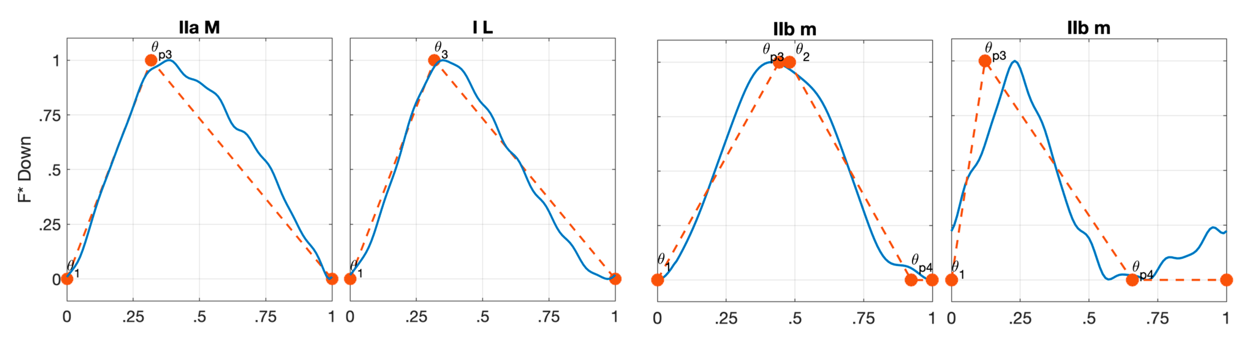
In Figure 9 cutting forces in both down-milling and up-milling, classified by the proposed approach as IIa type are shown in the three different configurations: no overlap, low overlap (L), and medium overlap (M). As in the previous cases, the proposed key points are in good agreement with the shape of the normalized cutting force, both in terms of error and shape. Higher error (around 10%) is found for the two IIa L configurations, probably because the noise in the force measurement is critical in normalizing cutting force with a large flat zone, leading to an underestimation of such zone with respect to the m value. However, as predicted by the proposed approach, a trapezoidal shape is found in no overlap and low overlap configuration, with the first characterized by an additional point. Starting from medium overlap the shape is characterized by two points, assuming a triangle-like shape as expected. Indeed, the high degree of overlap leads to the superimposition of the single flute profiles, generating this typical profile, as it is found in the experimental results and accurately predicted by the proposed formulations both in terms of angles and normalized magnitude.
Figure 10 shows the F shapes for type IIb in four different configurations, no overlap, low overlap (L) medium overlap (M), and deep medium overlap (m) for both down-milling (first row) and up-milling (second row). The comparison with the predicted shapes shows a very good match, with small deviations in down-milling for no overlap and low overlap. These deviations are found also in the error that in such configuration increase till almost 15%. The reason is the same presented for type IIa (i.e., noise influence in the normalization of the force) but increased since the flat zone in IIb is generally larger. Focusing on shape, for the first two overlap degrees same consideration of IIa type can be made regarding the trapezoidal-like shape of forces. Increasing the degree of overlap, different configurations can be found. Indeed, for M overlap in up-milling Equation (19) is verified and an additional key point (ϑf1) is found and predicted (Table 4). Likewise, for the m overlap, engagement conditions in down-milling ensure the presence of two additional points (ϑ2 ϑp4) because both Equations (20) and (21) are verified, while in up-milling only additional ϑf1 is predicted since only Equation (20) is verified. The predicted profiles are validated by the experimental results both for angles and normalized magnitude. F shapes for type III in three different configurations (no overlap, L and M overlaps) are presented in Figure 11. Since low ap is adopted in these configurations, a lower signal-to-noise ratio in the cutting forces is experienced and the formulations are found less accurate than the other types (average error of 13% with peak to over 20%). However, experimental forces fairly agree with the predicted key points. Indeed, it must be noted that the points ϑ3 in down-milling and ϑ2 in up-milling are expected to be at a lower magnitude position with respect to ϑM, as explained in Section 2.1, and this causes an increase of the computed error. Moreover, with high ar, such as the one characterizing the III type, a high curvature in falling (down-milling) or rising (up-milling) edges is expected.
In the no overlap configuration four points are predicted, since the engagement configuration is close to L overlap, the portion of engagement angle corresponding to no cutting is small, especially in up-milling, resulting in high proximity of points (ϑ1 and ϑ4). In the L overlap configuration three points are defined by the proposed formulations and accurately found in the experimental cutting forces, considering the expected discrepancy in terms of magnitude for ϑ3 in down-milling and ϑ2 in up-milling (as in Figure 3) with respect to ϑM. Experimental results for M configurations (tests 29 and 32) confirm the proposed key points, presenting a triangular shape deformed by the high curvature of the falling (down-milling) or rising (up-milling) edge, as expected.
Finally, in Figure 12 two noteworthy comparisons are presented: test 15 with test 33 and test 22 with test 34. In the first comparison (left side in Figure 12), two tests with a different axial depth of cut, type, and overlap but the same radial depth of cut are presented. Although very different, they present the same key points. Indeed, it must be pointed out that, according to the proposed formulations, the same predicted key points can be achieved by increasing the axial depth of the cut of specific values. Of course, experimental cutting forces are not the same in the two cases in terms of both force magnitude (the equivalence is valid for normalized values) and shape of the edges, as is clear from the figure and the previously described results. The second comparison (right side in Figure 12) presents the same type (IIb) and overlap (m) but with different engagement conditions, resulting in different cutting force profiles. This result confirms that the proposed formulations, as it is summarized in Table 3 for down-milling and Table 4 for up-milling, in a specific type and overlap combinations, include the potential occurrence of several points in the cutting force profile, but their presence depends on additional conditions Equations (18)–(21).
In summary, the experimental results show a good agreement with the proposed cutting force shape classification. Moreover, the experimental forces feature similar positions of key points compared to the ones expected. Small errors are found for type I, higher error for types II and III, for most of the results this is probably due to noise in the measurements that affect the normalization of forces and result in a high error, even if the shape was accurately estimated. Indeed, types II and III are characterized by higher depths of cut, resulting in higher forces and hence vibrations.
4. Conclusions
The total cutting force shape is not unique and varies according to cutting strategy, tool geometry, and cutting parameters. In this paper a comprehensive classification of total cutting force shape is presented, proposing four types of single-flute shape (I, IIa, IIb, III) and six configurations of overlap (no overlap, L, M, m, H, h). For each one of the types proposed, analytical formulations to predict force shape, as key points, are provided in terms of both key angles and the normalized magnitude value. The proposed formulations describe the normalized cutting forces (i.e., cutting force transformed in the maximum-minimum range, 0–1), at these characteristic points. These formulations, valid for the single-fluted endmill, are extended to a multiple-fluted endmill, by considering the different degrees of overlap. All the proposed formulations are based only on cutting strategy, tool geometry, and cutting parameters and do not require any cutting force model or cutting coefficients to be used. The main achieved results can be summarized in:
- A comprehensive model-independent classification of total cutting force shapes, including multi-flutes cutting simultaneously;
- Specific depths of cut conditions in which the different shapes occur;
- Analytical equations to predict key points of the total force shapes both in terms of key angles and magnitude;
- Thanks to the proposed formulations, it is possible to know in advance the expected shape of the cutting force without the need for any simulation or cutting force model.
The proposed method has been extensively validated through several milling tests in most of the conditions proposed by the classification. The results show a good agreement between the predicted key points and the actual ones on the measured cutting force profiles in all the tested types and overlaps combinations.
A potential application of such formulations could be the simulation or measurement of cutting forces only at the specific key angles, drastically reducing the time required for these tasks, still returning an accurate representation of the total cutting force.
Furthermore, the characteristic shape of the cutting force identified in this work could form the basis of a monitoring solution for the identification of engagement conditions in milling. However, it is highlighted that the key points of the normalized cutting forces are not unique for a specific set of cutting parameters, cutting strategy, and tool geometry since the same key points could be found in different conditions. Therefore, to fully take advantage of the proposed formulations for monitoring purposes it is suggested to include additional parameters, such as cutting force magnitude or shape characteristics (e.g., rising or falling edge curvature).
Author Contributions
Conceptualization and Methodology N.G., L.M., G.V.; Investigation and Validation N.G., L.M.; Writing—Original Draft N.G.; Writing—Review & Editing, G.V., L.M.; Supervision A.S., N.G.; Project administration and Funding acquisition, A.S. All authors have read and agreed to the published version of the manuscript.
Funding
The research received no external funding.
Data Availability Statement
No data are available but can be provided upon request.
Acknowledgments
The authors would like to thank Machine Tool Technology Research Foundation (MTTRF) and its supporters for the loaned machine tool (DMG MORI DMU 75 MonoBlock).
Conflicts of Interest
The authors declare no conflict of interest.
References
- Altintas, Y. Manufacturing Automation: Metal Cutting Mechanics, Machine Tool Vibrations, and CNC Design; Cambridge University Press: Cambridge, UK, 2012; ISBN 0521172470. [Google Scholar]
- Ambhore, N.; Kamble, D.; Chinchanikar, S.; Wayal, V. Tool condition monitoring system: A review. Mater. Today Proc. 2015, 2, 3419–3428. [Google Scholar] [CrossRef]
- Altintas, Y.; Yellowledy, I. The identification of radial width and axial depth of cut in peripheral milling. Int. J. Mach. Tools Manuf. 1987, 27, 367–381. [Google Scholar] [CrossRef]
- Kuljanic, E.; Sortino, M.; Totis, G. Multisensor approaches for chatter detection in milling. J. Sound Vib. 2008, 312, 672–693. [Google Scholar] [CrossRef]
- Schmitz, T.L.; Couey, J.; Marsh, E.; Mauntler, N.; Hughes, D. Runout effects in milling: Surface finish, surface location error, and stability. Int. J. Mach. Tools Manuf. 2007, 47, 841–851. [Google Scholar] [CrossRef]
- Liu, C.; Gao, L.; Wang, G.; Xu, W.; Jiang, X.; Yang, T. Online reconstruction of surface topography along the entire cutting path in peripheral milling. Int. J. Mech. Sci. 2020, 185, 105885. [Google Scholar] [CrossRef]
- Morelli, L.; Grossi, N.; Scippa, A.; Campatelli, G. Surface error shape identification for 3-axis milling operations. Procedia CIRP 2021, 101, 126–129. [Google Scholar] [CrossRef]
- Rubeo, M.A.; Schmitz, T.T.L. Mechanistic force model coefficients: A comparison of linear regression and nonlinear optimization. Precis. Eng. 2016, 45, 311–321. [Google Scholar] [CrossRef]
- Grossi, N. Accurate and fast measurement of specific cutting force coefficients changing with spindle speed. Int. J. Precis. Eng. Manuf. 2017, 1173–1180. [Google Scholar] [CrossRef]
- Lin, C.J.; Lui, Y.T.; Lin, Y.F.; Wang, H.B.; Liang, S.Y.; Wang, J.J.J. Prediction of shearing and ploughing constants in milling of inconel 718. J. Manuf. Mater. Process. 2021, 5, 8. [Google Scholar] [CrossRef]
- Kiran, K.; Kayacan, M.C. Cutting force modeling and accurate measurement in milling of flexible workpieces. Mech. Syst. Signal Process. 2019, 133, 106284. [Google Scholar] [CrossRef]
- Schmitz, T.L.; Mann, B.P. Closed-form solutions for surface location error in milling. Int. J. Mach. Tools Manuf. 2006, 46, 1369–1377. [Google Scholar] [CrossRef]
- Altintas, Y.; Budak, E. Analytical Prediction of Stability Lobes in Milling. CIRP Ann.-Manuf. Technol. 1995, 44, 357–362. [Google Scholar] [CrossRef]
- Sallese, L.; Innocenti, G.; Grossi, N.; Scippa, A.; Flores, R.; Basso, M.; Campatelli, G. Mitigation of chatter instabilities in milling using an active fixture with a novel control strategy. Int. J. Adv. Manuf. Technol. 2017, 89, 2771–2787. [Google Scholar] [CrossRef]
- Yun, W.S.; Ko, J.H.; Cho, D.W.; Ehmann, K.F. Development of a virtual machining system, Part 2: Prediction and analysis of a machined surface error. Int. J. Mach. Tools Manuf. 2002, 42, 1607–1615. [Google Scholar] [CrossRef]
- Scippa, A.; Montevecchi, F.; Grossi, N.; Sallese, L.; Campatelli, G. Time domain simulation model for active fixturing in milling. In Proceedings of the 8th International Conference on Leading Edge Manufacturing in 21st Century, LEM 2015, Kyoto, Japan, 18–22 October 2015. [Google Scholar]
- Gonzalo, O.; Beristain, J.; Jauregi, H.; Sanz, C. A method for the identification of the specific force coefficients for mechanistic milling simulation. Int. J. Mach. Tools Manuf. 2010, 50, 765–774. [Google Scholar] [CrossRef]
- Ducroux, E.; Fromentin, G.; Viprey, F.; Prat, D.; D’Acunto, A. New mechanistic cutting force model for milling additive manufactured Inconel 718 considering effects of tool wear evolution and actual tool geometry. J. Manuf. Process. 2021, 64, 67–80. [Google Scholar] [CrossRef]
- Hwang, J.H.; Oh, Y.T.; Kwon, W.T.; Chu, C.N. In-process estimation of radial immersion ratio in face milling using cutting force. Int. J. Adv. Manuf. Technol. 2003, 22, 313–320. [Google Scholar] [CrossRef]
- Lin, C.-Y.; Yeh, S.-S. Integration of cutting force control and chatter suppression control into automatic cutting feed adjustment system design. Mach. Sci. Technol. 2020, 24, 65–95. [Google Scholar] [CrossRef]
- Leal-Muñoz, E.; Diez, E.; Perez, H.; Vizan, A. Accuracy of a new online method for measuring machining parameters in milling. Measurement 2018, 128, 170–179. [Google Scholar] [CrossRef]
- Bachrathy, D.; Insperger, T.; Stépán, G. Surface properties of the machined workpiece for helical mills. Mach. Sci. Technol. 2009, 13, 227–245. [Google Scholar] [CrossRef]
- Wang, J.-J.J.; Liang, S.Y.; Book, W.J. Convolution Analysis of Milling Force Pulsation. J. Eng. Ind. 1994, 116, 17–25. [Google Scholar] [CrossRef]
- Dhupia, J.; Girsang, I. Correlation-based estimation of cutting force coefficients for ball-end milling. Mach. Sci. Technol. 2012, 16, 287–303. [Google Scholar] [CrossRef]
- Prickett, P.W.; Siddiqui, R.A.; Grosvenor, R.I. The development of an end-milling process depth of cut monitoring system. Int. J. Adv. Manuf. Technol. 2011, 52, 89–100. [Google Scholar] [CrossRef]
- Morelli, L.; Grossi, N.; Scippa, A.; Campatelli, G. Extended classification of surface errors shapes in peripheral end-milling operations. J. Manuf. Process. 2021, 71, 604–624. [Google Scholar] [CrossRef]
- Choi, J.G.; Yang, M.Y. In-process prediction of cutting depths in end milling. Int. J. Mach. Tools Manuf. 1999, 39, 705–721. [Google Scholar] [CrossRef]
- Yang, L.; DeVor, R.E.; Kapoor, S.G. Analysis of Force Shape Characteristics and Detection of Depth-of-Cut Variations in End Milling. J. Manuf. Sci. Eng. 2004, 127, 454–462. [Google Scholar] [CrossRef]
- Islam, M.N.; Lee, H.U.; Cho, D.W. Prediction and analysis of size tolerances achievable in peripheral end milling. Int. J. Adv. Manuf. Technol. 2008, 39, 129–141. [Google Scholar] [CrossRef]
- Desai, K.A.; Rao, P.V.M. On cutter deflection surface errors in peripheral milling. J. Mater. Process. Technol. 2012, 212, 2443–2454. [Google Scholar] [CrossRef]
- Scippa, A.; Sallese, L.; Grossi, N.; Campatelli, G. Improved dynamic compensation for accurate cutting force measurements in milling applications. Mech. Syst. Signal Process. 2015, 54–55, 314–324. [Google Scholar] [CrossRef]
- Totis, G.; Sortino, M. Upgraded Regularized Deconvolution of complex dynamometer dynamics for an improved correction of cutting forces in milling. Mech. Syst. Signal Process. 2022, 166, 108412. [Google Scholar] [CrossRef]
- Magnevall, M.; Lundblad, M.; Ahlin, K.; Broman, G. High frequency measurements of cutting forces in milling by inverse filtering. Mach. Sci. Technol. 2012, 16, 487–500. [Google Scholar] [CrossRef]
Figure 1.
Schematic diagram of milling parameters: (a) Down-milling (b) Up-milling.

Figure 2.
Schematic diagram of cutting edge’ locations during the cutting process (black dashed lines represent the cutting edge at the different key positions).
Figure 2.
Schematic diagram of cutting edge’ locations during the cutting process (black dashed lines represent the cutting edge at the different key positions).
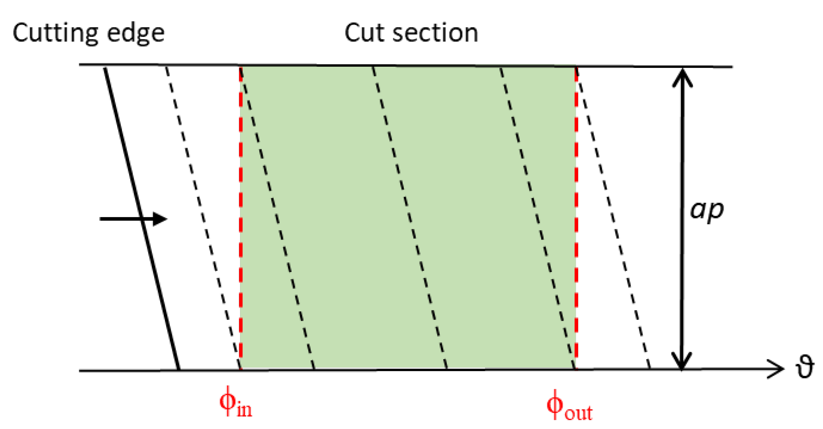
Figure 3.
Examples of single flute F shapes in one period (a) Down-milling (ϑ1; ϑ1 + ϕz) (b) Up-milling (ϑ4 − ϕz; ϑ4).
Figure 3.
Examples of single flute F shapes in one period (a) Down-milling (ϑ1; ϑ1 + ϕz) (b) Up-milling (ϑ4 − ϕz; ϑ4).
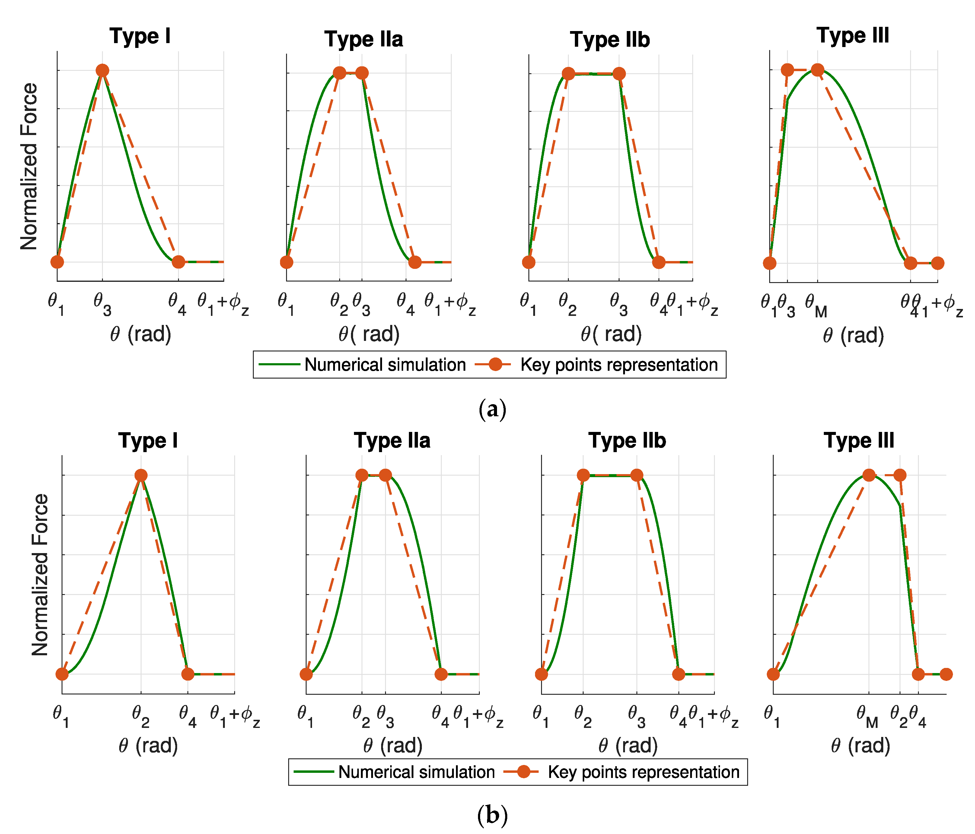
Figure 4.
Example of multiple flutes endmill F shape for both down-milling and up-milling.
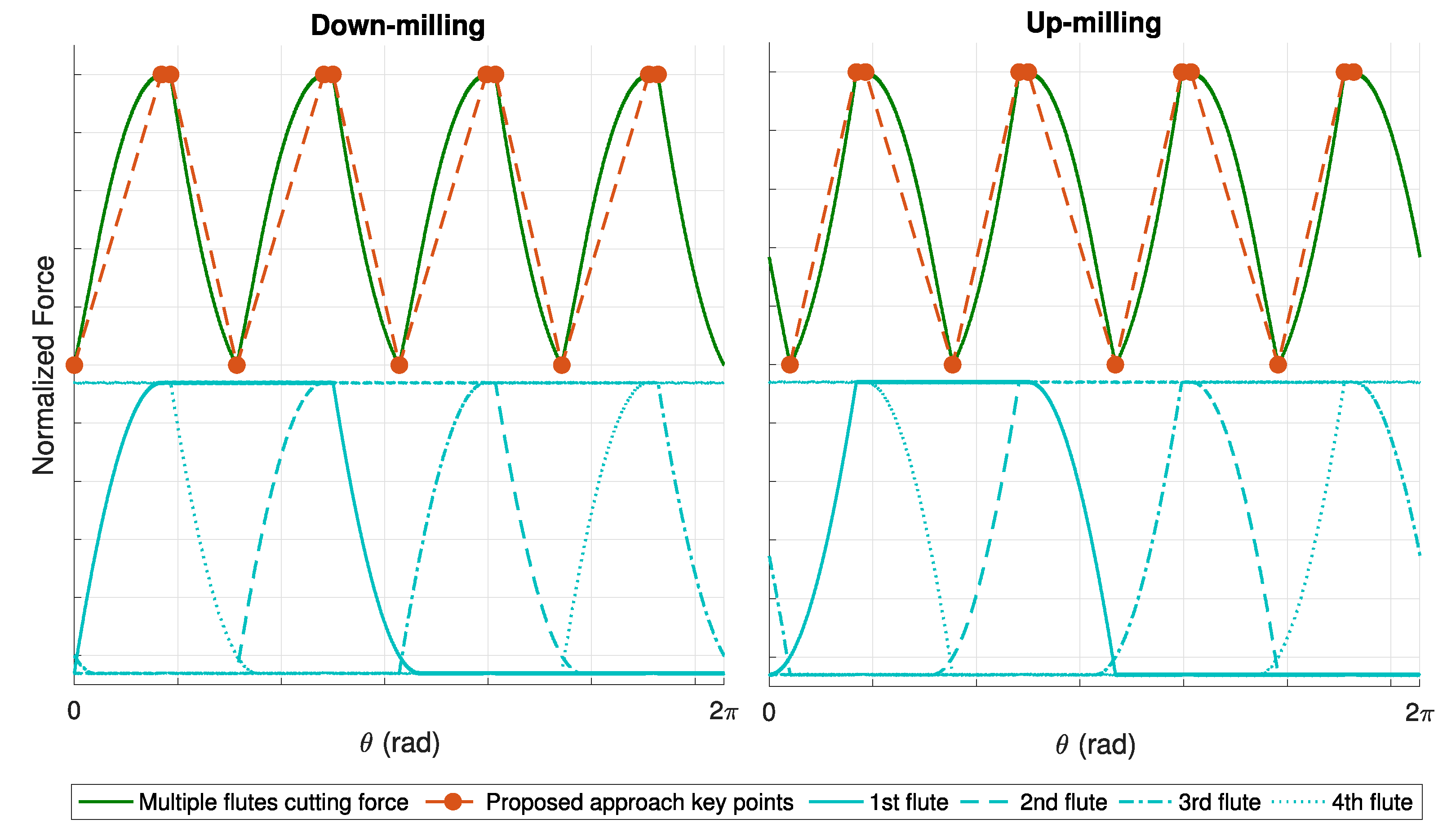
Figure 5.
Example of different degrees of overlap for different types of single flute F shape in down-milling.
Figure 5.
Example of different degrees of overlap for different types of single flute F shape in down-milling.

Figure 6.
(a) experimental set-up (b) tool 1 (c) tool 2.
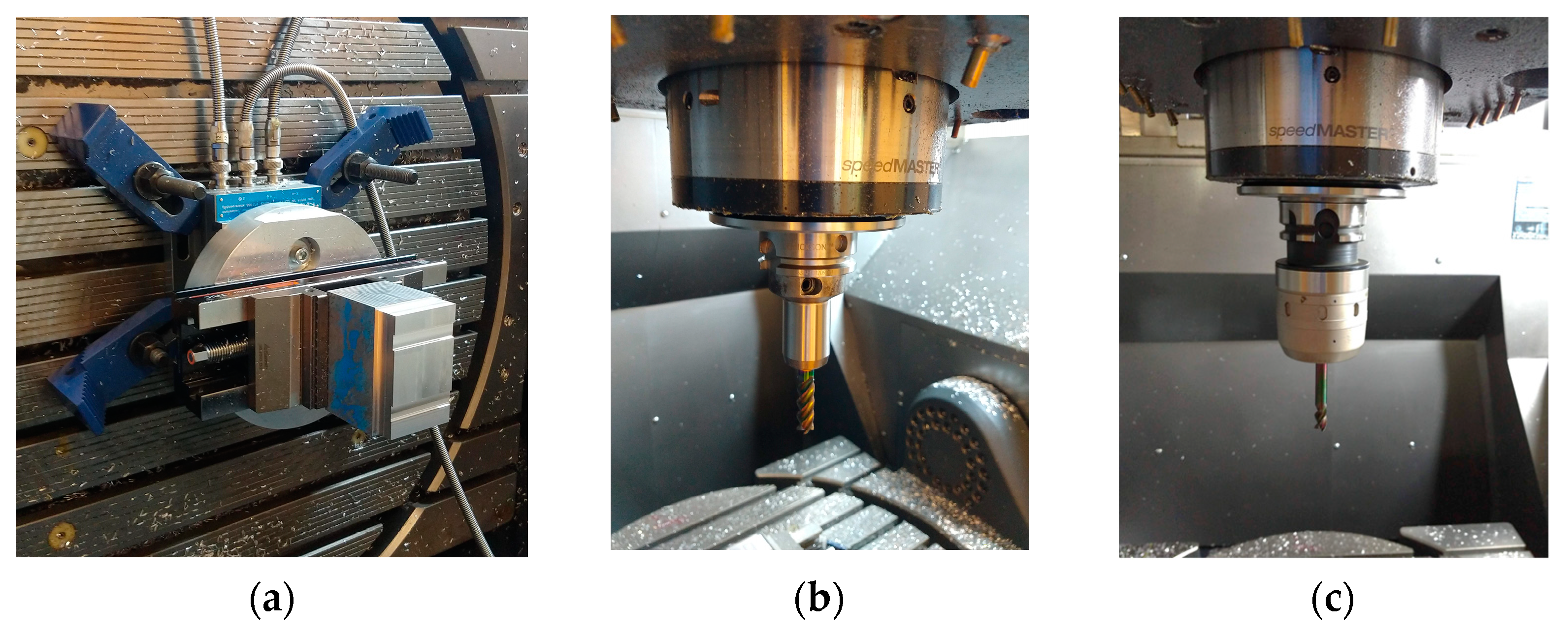
Figure 7.
Type I normalized F shapes for tool 1 (tests 1 to 4 in down-milling; tests 5 to 8 in up-milling).
Figure 7.
Type I normalized F shapes for tool 1 (tests 1 to 4 in down-milling; tests 5 to 8 in up-milling).
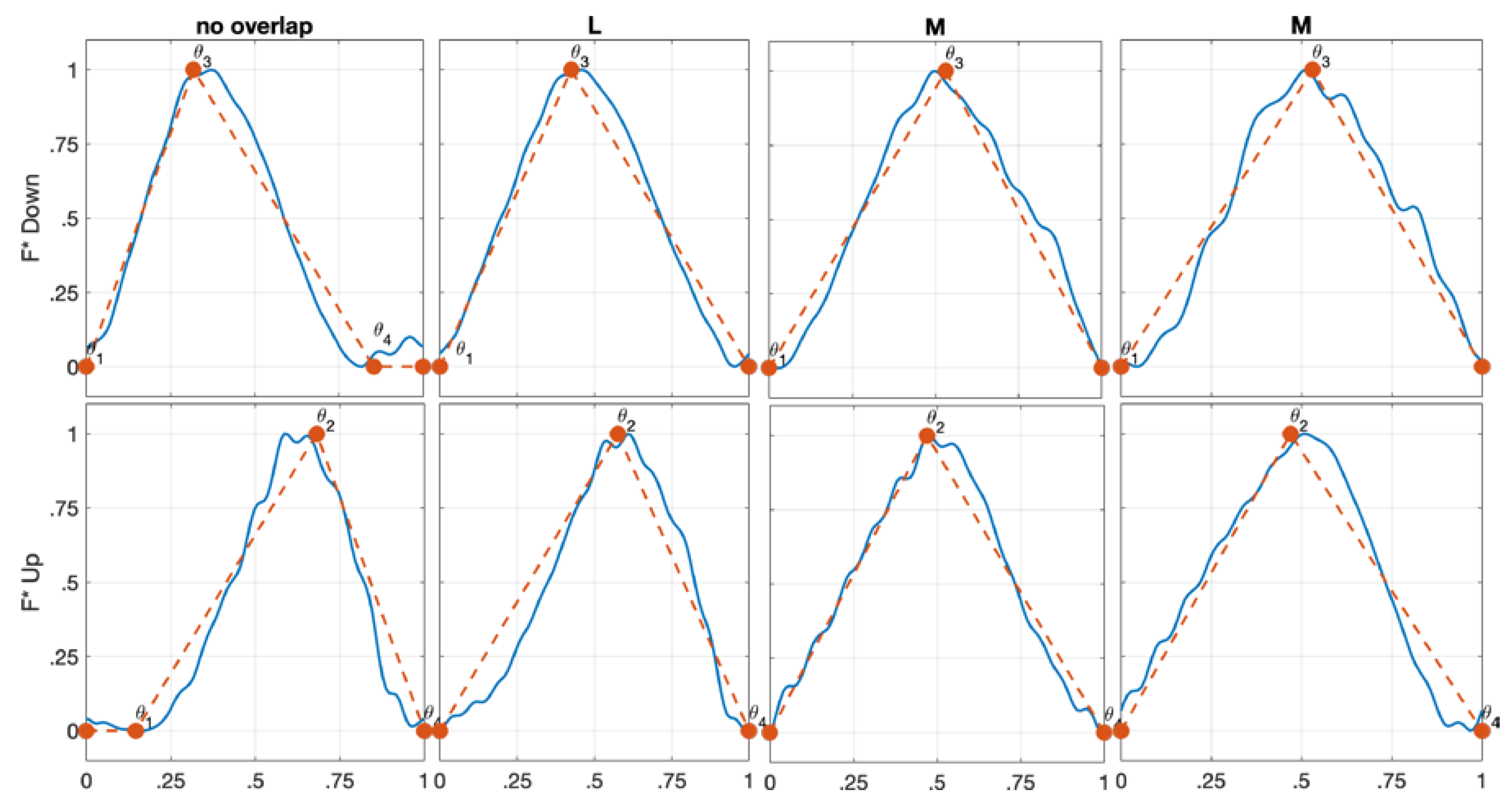
Figure 8.
Type I normalized F shapes for tool 2 (tests 7 to 9 in down-milling; tests 10 to 12 in up-milling).
Figure 8.
Type I normalized F shapes for tool 2 (tests 7 to 9 in down-milling; tests 10 to 12 in up-milling).
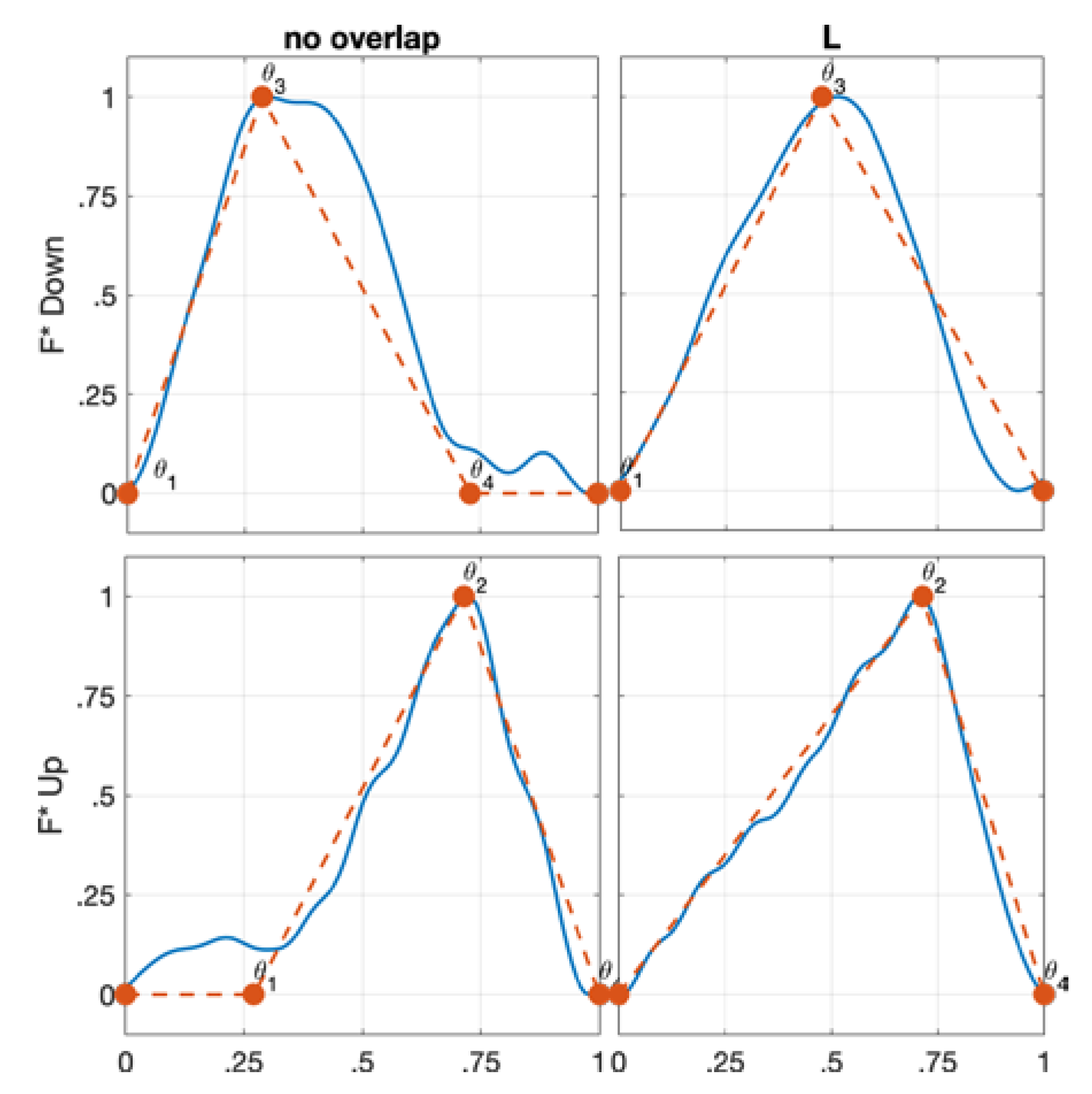
Figure 9.
Type IIa normalized F shapes (tests 13 to 15 in down-milling; tests 16 to 18 in up-milling).
Figure 9.
Type IIa normalized F shapes (tests 13 to 15 in down-milling; tests 16 to 18 in up-milling).
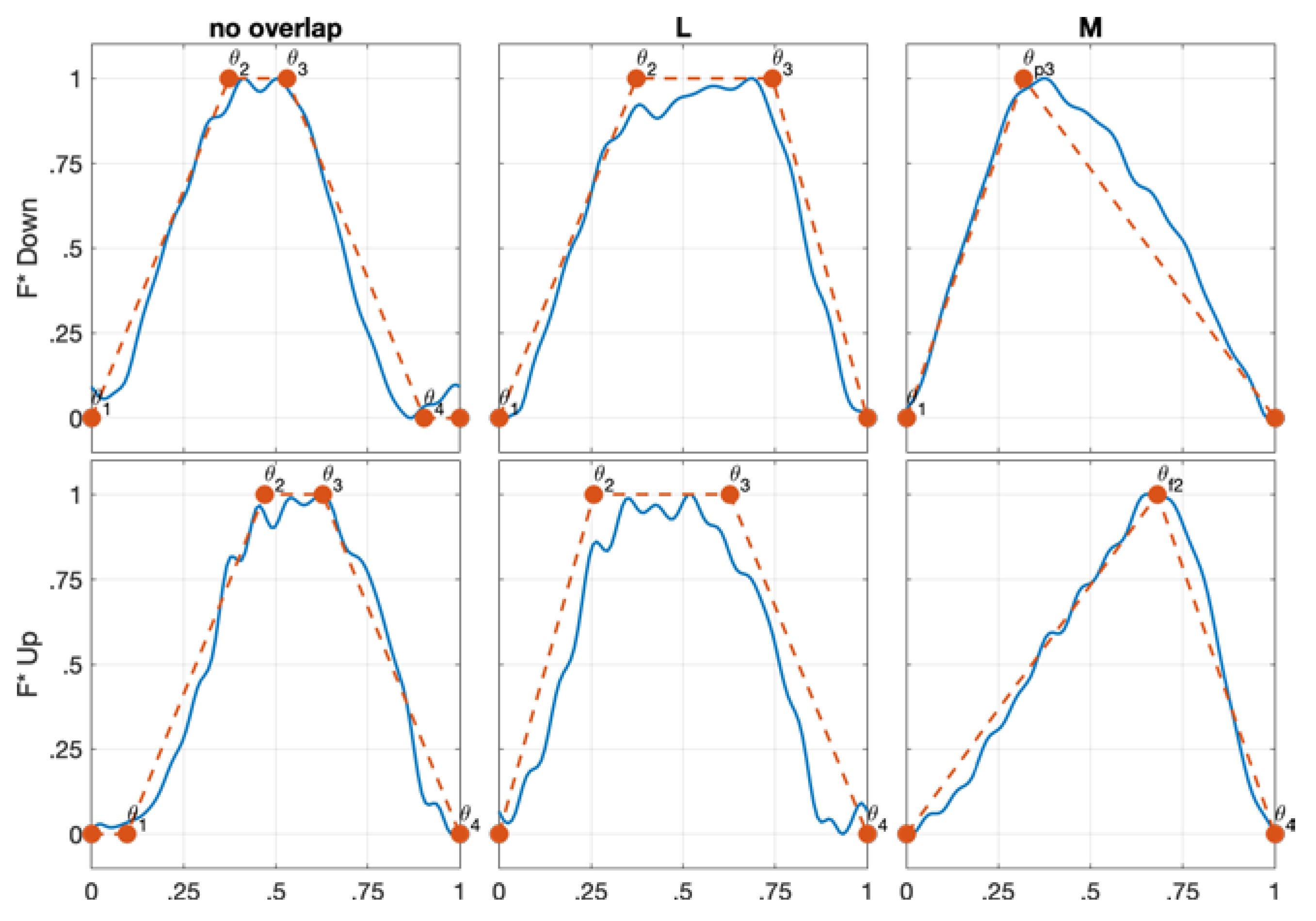
Figure 10.
Type IIb normalized F shapes (tests 19 to 22 in down-milling; tests 23 to 26 in up-milling).
Figure 10.
Type IIb normalized F shapes (tests 19 to 22 in down-milling; tests 23 to 26 in up-milling).
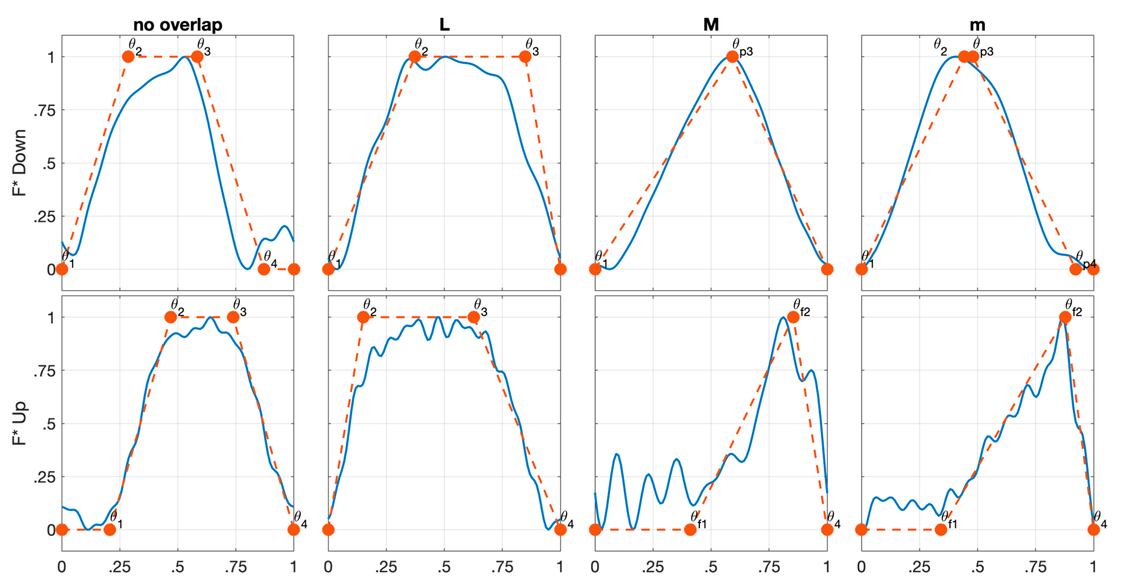
Figure 11.
Type III normalized F shapes (tests 27 to 29 in down-milling; tests 30 to 32 in up-milling).
Figure 11.
Type III normalized F shapes (tests 27 to 29 in down-milling; tests 30 to 32 in up-milling).
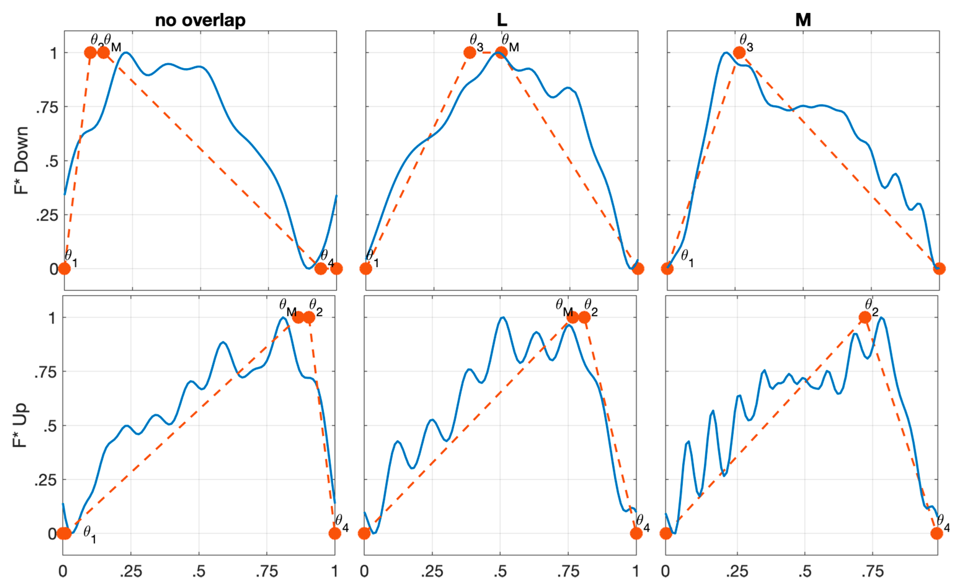
Figure 12.
Normalized total forces comparison: test 15 vs. 33; test 22 vs. 34.

Table 1.
Single flute F type conditions.
| I | IIa | IIb | III | |
|---|---|---|---|---|
| Down-milling | αen < αenc αsw ≤ αswc | αen < αenc αsw > αswc αen < 2αswc | αen < αenc αsw > αswc αen ≥ 2αswc | αen ≥ αenc αsw ≤ αswc |
| Up-milling | αen ≤ αenc αsw ≤ αswc | αen < αenc αsw > αswc αen < 2αswc | αen < αenc αsw > αswc αen ≥ 2αswc | αen ≥ αenc αsw ≤ αswc |
Table 2.
Single flute F type key points.
| I | IIa | IIb | III | |
|---|---|---|---|---|
| Down-milling | (ϑ1; 0) (ϑ3; 1) (ϑ4; 0) | (ϑ1; 0) (ϑ2; 1) (ϑ3; 1) (ϑ4; 0) | (ϑ1; 0) (ϑ2; 1) (ϑ3; 1) (ϑ4; 0) | (ϑ1; 0) (ϑ3; 1) (ϑM; 1) (ϑ4; 0) |
| Up-milling | (ϑ1; 0) (ϑ2; 1) (ϑ4; 0) | (ϑ1; 0) (ϑ2; 1) (ϑ3; 1) (ϑ4; 0) | (ϑ1; 0) (ϑ2; 1) (ϑ3; 1) (ϑ4; 0) | (ϑ1; 0) (ϑM; 1) (ϑ2; 1) (ϑ4; 0) |
Table 3.
Multiple flutes F shape key points for one period (ϑ1; ϑ1 + ϕz) in down-milling.
| I | IIa | IIb | III | |
|---|---|---|---|---|
| No Overlap | (ϑ1; 0) (ϑ3; 1) (ϑ4; 0) | (ϑ1; 0) (ϑ2; 1) (ϑ3; 1) (ϑ4; 0) | (ϑ1; 0) (ϑ2; 1) (ϑ3; 1) (ϑ4; 0) | (ϑ1; 0) (ϑ3; 1) (ϑM; 1) (ϑ4; 0) |
| Low (L) | (ϑ1; 0) (ϑ3; 1) | (ϑ1; 0) (ϑ2; 1) (ϑ3; 1) | (ϑ1; 0) (ϑ2; 1) (ϑ3; 1) | (ϑ1; 0) (ϑ3; 1) (ϑM; 1) |
| Medium (M) | (ϑ1; 0) (ϑ3; 1) | (ϑ1; 0) (ϑp3; 1) (ϑp4; 0) if (18) | (ϑ1; 0) (ϑp3; 1) (ϑp4; 0) if (18) | (ϑ1; 0) (ϑ3; 1) |
| High (H) | (ϑ1; 0) (ϑp3; 1) | (ϑ1; 0) (ϑp3; 1) | n/a | (ϑ1; 0) (ϑp3; 1) |
| Deep medium (m) | n/a | n/a | (ϑ1; 0) (ϑ2; 1) if (20) (ϑp3; 1) (ϑp4; 0) if (19) | n/a |
| Deep high (h) | n/a | (ϑ1; 0) (ϑp3; 1) | (ϑ1; 0) (ϑp3; 1) | n/a |
Table 4.
Multiple flutes F shape key points for one period (ϑ4 − ϕz; ϑ4) in up-milling.
| I | IIa | IIb | III | |
|---|---|---|---|---|
| No Overlap | (ϑ1; 0) (ϑ2; 1) (ϑ4; 0) | (ϑ1; 0) (ϑ2; 1) (ϑ3; 1) (ϑ4; 0) | (ϑ1; 0) (ϑ2; 1) (ϑ3; 1) (ϑ4; 0) | (ϑ1; 0) (ϑM; 1) (ϑ2; 1) (ϑ4; 0) |
| Low (L) | (ϑ2; 1) (ϑ4; 0) | (ϑ2; 1) (ϑ3; 1) (ϑ4; 0) | (ϑ2; 1) (ϑ3; 1) (ϑ4; 0) | (ϑM; 1) (ϑ2; 1) (ϑ4; 0) |
| Medium (M) | (ϑ2; 1) (ϑ4; 0) | (ϑf1; 1) if (18) (ϑf2; 1) (ϑ4; 0) | (ϑf1; 1) if (18) (ϑf2; 1) (ϑ4; 0) | (ϑ2; 1) (ϑ4; 0) |
| High (H) | (ϑf2; 1) (ϑ4; 0) | (ϑf2; 1) (ϑ4; 0) | n/a | (ϑ2; 1) (ϑ4; 0) |
| Deep medium (m) | n/a | n/a | (ϑf1; 1) if (19) (ϑf2; 1) (ϑ3; 1) if (21) (ϑ4; 0) | n/a |
| Deep high (h) | n/a | (ϑ1; 0) (ϑp3; 1) | (ϑ1; 0) (ϑp3; 1) | n/a |
Table 5.
Endmill parameters.
| Endmill | Tool ID | D (mm) | N | αhel (deg) | Cutting Length (mm) | fz (mm/Flute) | Spindle Speed (rpm) |
|---|---|---|---|---|---|---|---|
| 202552 | 1 | 12 | 4 | 45 | 36 | 0.1 | 6366 |
| 202274 | 2 | 10 | 3 | 45 | 16 | 0.04 | 12,732 |
Table 6.
Milling tests overview.
| Test | Type | Overlap | Strategy | Tool ID | ar (mm) | ap (mm) | Error (%) |
|---|---|---|---|---|---|---|---|
| 1 | I | No Overlap | Down | 1 | 2 | 3 | 4.2 |
| 2 | I | Low | Down | 1 | 3 | 4 | 3.3 |
| 3 | I | Medium | Down | 1 | 6 | 5 | 4.1 |
| 4 | I | Medium | Down | 1 | 6.5 | 5 | 1.9 |
| 5 | I | No Overlap | Up | 1 | 2 | 3 | 2.8 |
| 6 | I | Low | Up | 1 | 3 | 4 | 2.6 |
| 7 | I | Medium | Up | 1 | 6 | 5 | 0.1 |
| 8 | I | Medium | Up | 1 | 6.5 | 5 | 4.9 |
| 9 | I | No Overlap | Down | 2 | 2 | 3 | 3.9 |
| 10 | I | Low | Down | 2 | 3 | 5 | 2.1 |
| 11 | I | No Overlap | Up | 2 | 2 | 3 | 4.7 |
| 12 | I | Low | Up | 2 | 3 | 5 | 0.1 |
| 13 | IIa | No Overlap | Down | 1 | 1 | 5 | 5.2 |
| 14 | IIa | Low | Down | 1 | 1 | 7 | 6.8 |
| 15 | IIa | Medium | Down | 1 | 4 | 12.4 | 2.9 |
| 16 | IIa | No Overlap | Up | 1 | 1 | 5 | 4.2 |
| 17 | IIa | Low | Up | 1 | 1 | 7 | 9.8 |
| 18 | IIa | Medium | Up | 1 | 4 | 12.4 | 0.4 |
| 19 | IIb | No Overlap | Down | 1 | 0.6 | 5.5 | 13.7 |
| 20 | IIb | Low | Down | 1 | 1 | 8 | 17.1 |
| 21 | IIb | Medium | Down | 1 | 2.5 | 15 | 1.4 |
| 22 | IIb | Deep Medium | Down | 2 | 2 | 15 | 2.7 |
| 23 | IIb | No Overlap | Up | 1 | 0.5 | 5 | 9.5 |
| 24 | IIb | Low | Up | 1 | 1 | 8 | 14.1 |
| 25 | IIb | Medium | Up | 2 | 2 | 12 | 12.1 |
| 26 | IIb | Deep Medium | Up | 1 | 2 | 20 | 3.0 |
| 27 | III | No Overlap | Down | 2 | 6 | 1 | 25.3 |
| 28 | III | Low | Down | 2 | 8 | 4 | 6.3 |
| 29 | III | Medium | Down | 1 | 7.5 | 2.5 | 2.8 |
| 30 | III | No Overlap | Up | 2 | 6.5 | 1 | 18.5 |
| 31 | III | Low | Up | 2 | 7 | 2 | 11.0 |
| 32 | III | Medium | Up | 1 | 7.5 | 2.5 | 12.7 |
| 33 | I | Low | Down | 1 | 4 | 3 | 2.2 |
| 34 | IIb | Deep Medium | Down | 1 | 2 | 20 | 19.7 |
Publisher’s Note: MDPI stays neutral with regard to jurisdictional claims in published maps and institutional affiliations. |
© 2021 by the authors. Licensee MDPI, Basel, Switzerland. This article is an open access article distributed under the terms and conditions of the Creative Commons Attribution (CC BY) license (https://creativecommons.org/licenses/by/4.0/).
Share and Cite
MDPI and ACS Style
Grossi, N.; Morelli, L.; Venturini, G.; Scippa, A. Forces Shapes in 3-Axis End-Milling: Classification and Characteristic Equations. J. Manuf. Mater. Process. 2021, 5, 117. https://doi.org/10.3390/jmmp5040117
AMA Style
Grossi N, Morelli L, Venturini G, Scippa A. Forces Shapes in 3-Axis End-Milling: Classification and Characteristic Equations. Journal of Manufacturing and Materials Processing. 2021; 5(4):117. https://doi.org/10.3390/jmmp5040117
Chicago/Turabian StyleGrossi, Niccolò, Lorenzo Morelli, Giuseppe Venturini, and Antonio Scippa. 2021. "Forces Shapes in 3-Axis End-Milling: Classification and Characteristic Equations" Journal of Manufacturing and Materials Processing 5, no. 4: 117. https://doi.org/10.3390/jmmp5040117