
Tool Wear Monitoring with Artificial Intelligence Methods: A Review


1
Department of Mechanical and Industrial Engineering, University of Brescia, Via Branze 38, 25123 Brescia, Italy
2
Department of Engineering for Innovation, University of Salento, Via per Monteroni, 73100 Lecce, Italy
*
Author to whom correspondence should be addressed.
J. Manuf. Mater. Process. 2023, 7(4), 129; https://doi.org/10.3390/jmmp7040129
Submission received: 12 May 2023
/
Revised: 2 July 2023
/
Accepted: 6 July 2023
/
Published: 11 July 2023
(This article belongs to the Special Issue Industry 4.0 and Smart Materials Processing for Enhanced Manufacturing)
Abstract
:Tool wear is one of the main issues encountered in the manufacturing industry during machining operations. In traditional machining for chip removal, it is necessary to know the wear of the tool since the modification of the geometric characteristics of the cutting edge makes it unable to guarantee the quality required during machining. Knowing and measuring the wear of tools is possible through artificial intelligence (AI), a branch of information technology that, by interpreting the behaviour of the tool, predicts its wear through intelligent systems. AI systems include techniques such as machine learning, deep learning and neural networks, which allow for the study, construction and implementation of algorithms in order to understand, improve and optimize the wear process. The aim of this research work is to provide an overview of the recent years of development of tool wear monitoring through artificial intelligence in the general and essential requirements of offline and online methods. The last few years mainly refer to the last ten years, but with a few exceptions, for a better explanation of the topics covered. Therefore, the review identifies, in addition to the methods, the industrial sector to which the scientific article refers, the type of processing, the material processed, the tool used and the type of wear calculated. Publications are described in accordance with PRISMA-P (Preferred Reporting Items for Systematic review and Meta-Analysis Protocols).
1. Introduction
Tool condition monitoring is a key component of micromachining, macromachining and modern industry. Sectors such as aeronautics, aerospace, energy and electricity frequently encounter materials that are more or less difficult to operate by conventional cutting. The purpose of tool monitoring is to improve product quality, reduce costs and maximise productivity.
From an economic point of view, Zhang et al. [1] stated that about 3–12% of the production cost is related to the condition of the cutting tools and their replacement. Therefore, the development of a Tool Condition Monitoring (TCM) system is essential to effectively and efficiently understand the condition of cutting tools in order to predict and optimize their lifetime. From [2,3], it can be summarized that an accurate and reliable TCM system could generate a 10–50% increase in cutting speed, a 75% reduction in downtime and a maintenance cost saving of approximately 30% [4,5].
Today, especially in consolidated technologies such as turning, milling and drilling, the maximum cost reduction is sought to be competitive in the marketplace. In a shop floor, the processing cycle of products is divided into several processing phases. The processing phases include milling, drilling and turning. For each phase, different tools are used that tend to wear out over time. Each processing phase has a specific production time. The sum of the times of the working phases identifies the lead time of products. Consequently, a premature failure of one or more tools results in a loss of machine downtime, which affects the productivity, quality and execution time of the products.
Industry 4.0, through its technologies such as intelligent sensors, signal acquisition, data analysis and AI, can reduce or avoid these unexpected failures. Tool condition monitoring (TCM) is a technique that has been studied for many years and publications have shown how an accurate and correct result can be obtained in a single operation. However, in today’s marketplace, a full and efficient TCM can rarely reliably perform all functions.
Therefore, transferring these results to the industrial world is not always simple and immediate, especially since in recent years the industrial world has increasingly focused on varied and diversified products in almost all sectors, creating a continuous change in production. Predicting tool wear and residual life is very difficult, but once a possible solution has been found, it can significantly reduce downtime, loss and cost.
The purpose of this document is to present a review of instrument monitoring systems over the last 10 years, from 2010 to 2022, with some exceptions, according to the PRISMA-P checklist [6].
The objective of the review is to identify the methods of research used from 2010 to 2022 to improve tool wear monitoring through AI methods.
Checklist review writing points are objectives, eligibility criteria, sources of information, search strategy, study articles, data elements, results and priority setting; Summary of Data. Checklist details can be found in “Appendix A”.
The questions that the review asks to identify all of the features of tool wear monitoring through artificial intelligence methods are:
- (1)
- Which publications simultaneously use offline and online measurement methods to detect tool wear?
The next questions include, as a fundamental point, whether the publications considered have a comparison between the offline and online methods of measuring tool wear. Otherwise, they are not taken into account.
- (2)
- What are the cutting parameters used? What types of tools are used in milling, turning and drilling? What are the turning, milling and drilling machine tools used? What are the metal materials processed?
- (3)
- Which sensors can detect and interpret these signals in milling, drilling and turning processes?
- (4)
- What are the characteristics that can be extracted in the time domain, frequency domain and time-frequency domain? Are we also using raw data, or other signal signals?
- (5)
- What are the artificial intelligence algorithms that predict tool wear?
- (6)
- What are the performances that use algorithms to predict tool wear?
- (7)
- What is the value of the performances that use the algorithms to see the tool wear?
2. Methods of Research Level, Research Item and Research Number of Published Articles Found
Eligibility Criteria and Search Strategy
The included articles were reviewed and published in international classified journals. They had a release date ranging from 2010 to 2020, with some exceptions. The searches carried out indicated the title of the research, the years of publication and the research field. Table 1 shows the search strategies adopted. Five levels of research were defined with different searching rules (i.e., ITEMS). In this way, from 21,760 articles, 77 were selected as the more important.
3. Selection of Offline and Online Publications and Related Data Extraction from the Publications
A standard electronic data collection form was used for data extraction. The 77 items selected, as shown in Table 1, contain numerous data that characterise the method used to calculate tool wear. The data may be the type of tool wear calculated, the machine tool used, the cutting parameters in the mechanical processing or the type of tool used to perform the mechanical processing. To identify and explain the data for the 77 items, we defined the flowchart shown in Figure 1. The choice of data in the sections was divided into two parts. The first part indicated the general and essential requirements for monitoring tool wear: (1) type of mechanical processing; (2) type of tool; (3) type of wear; (4) type of machine tool; (5) type of processed material; (6) industrial sector concerned. The second part showed the comparative methods used to calculate tool wear. Two methods were identified, one offline and one online. In the offline method, the data were: (1) cutting parameters; (2) wear calculation equipment. In the online method, in addition to considering the offline data, there were: (1) the tool wear prediction algorithm; (2) the data acquisition method (sensor); (3) the data acquisition hardware system; (4) feature extraction of the sensor signal and performances of AI; (5) software used for AI; (6) the industrial sector.
Each variable indicated in the flowchart in Figure 1 specifies that the selection of the articles, and thus the extraction of the data from them, was performed through certain characteristics. For mechanical processing, turning, milling or drilling operations were specified; for the type of tool, the technical characteristics of the tool, such as the diameter, the material, the coating and the type of ISO 1832 [7]. classification were indicated; for the type of tool wear, the wear on the flank (VB), the depth of the wear crater (KT), the surface area of the wear (S), the radial wear (RW), the wear of the diameter (DW), the RUL (tool remaining useful life), the tool wear rate and the flank wear width (FWW) were reported; for the type of machine tool, the type of machine tool used to carry out the experiment was indicated, such as a lathe, a milling machine or a drilling machine; for the type of material, the workpiece on which the milling, turning and drilling operations are performed was indicated; for the type of industrial sector, the area in which the research had been applied or could be applied in the future was indicated.
Tool wear is calculated using two measurement methods: the static offline method and the dynamic inline method. The term static refers to the ability to measure and visualize the trend of tool wear immediately after the production of a predefined number of parts. This means stopping the process for a while and then rebooting it. Otherwise, dynamic methods constantly measure tool wear without stopping the process. The measurement can be directly (by means of vision sensors) or indirectly made by measuring vibration or forces. Sensor signals are fed into an algorithm that predicts future tool wear. Prediction continuously improves over time.
The variables entered in the online method, as indicated in the flow diagram in Figure 1, were: the algorithm indicates the type of algorithm used to predict the wear of the instrument, such as the K-stellar algorithm; the data acquisition method indicates the type of sensors used to acquire signal changes during mechanical processing. Sensors can include dynamometers, accelerometers and acoustic emission sensors. The dynamometer measures force, the acoustic emission sensor measures sound and the accelerometer measures vibration. The hardware data acquisition system specifies the type of hardware system for the acquisition of sensor data during processing. It can consist of a PC and a data acquisition device; the extraction characteristics of the signal sensor indicate the fundamental characteristics, such as the mean, variance and RMS of the analysed data, while performance indicates the quality of the algorithm AI for the calculation of wear. Usually, before the construction phase of an AI model, the dataset is analysed and manipulated to extract significant properties from those already available. This process is called feature extraction and plays a critical role in creating a robust machine learning strategy. Software algorithm means the name of the software used to run the algorithm. Examples of software are MATLAB, tensorflow and Roboream; the industry sector indicates whether the experience identified in the article can be applied in an industrial context and with what accuracy.
4. Results of Research
4.1. Introduction Selection and Inclusion of Publications
After the screening of 21,760 publications, 2959 were recovered and codified. Without considering the microcuttings, 116 articles were identified. Of these 116 articles, 97 involved calculating tool wear using AI for micromachining, such as turning, drilling and milling. The acquisition of signals through cameras and optical systems was not considered. Subsequently, 77 articles were identified as being suitable for the inclusion criteria. For further details on the selection of the articles, Table 1 shows all specifications.
4.2. General and Essential Requirement of Machining Operations, Number of Articles, Type of Wear, Type of Machine and Type of Material
Of the seventy-seven articles selected, fifty-one related to milling, nineteen related to turning, five related to drilling and two related to all three processes. Three types of cutters were identified in the milling process: insert mills with hard metal inserts, solid carbide mills and solid mills in high-speed steel. Two types of tools were identified in the drilling process: solid carbide drills and solid high-speed steel drills. CNMG inserts tended to be used in the turning process. The inserts used were 95% coated hard metal and 5% ceramic. The wears calculated on the tools were the flank wear, the RUL and the tool wear rate. The machines used were vertical milling machines, vertical drilling machines and traditional lathes. The materials processed by the machine tools with the related tools were: cast irons, steel alloys, super alloys and aluminium alloys. In steel alloys were machined: C45, stainless steel (such as AISI 316), 42CrMo4, S235JR, 1018 steel, 1040 steel, mild steel, tempered steel and AISI M3: 2. Super alloys are machined titanium alloys, Inconel 718 and Inconel 625. Aluminium alloys are machined aluminium 6061, 5053, 6082, 2024, 7022 and 7075. Table 2 shows the general and essential requirements.
4.3. Introduction Methods of Measurement
Tool wear is calculated using two measurements: the offline measurement, which is static, and the online measurement, which is dynamic. By comparing the two measurements, the tool wear can be calculated with greater accuracy. The diagram in Figure 2 [58] shows how to compare the two measurements. In the offline measurement, the machine performs the machining and, after a certain amount of workpieces or minutes worked, stops the machining and, through a microscope, the tool wear is measured. Wear is then measured until the tool is replaced because it is worn. In the online measurement during the operation of the machine, sensors inserted inside the machine detect the evolution of the wear of the tool. The sensors generate signals that are first translated by the data acquisition system and then analysed to create the correct dataset to be inserted into the AI. AI, through its intelligent algorithm, predicts the wear trend of tools. The correct comparison between the two measurements predicts the wear of the tool with great accuracy. All seventy-seven selected articles compared the two measurements. The differences are in terms of the process, the cutting parameters, the type of microscope, the sensors used, the data acquisition system and the AI algorithm.
4.3.1. Offline Measurement
The machine tool performs the operations of milling, drilling or turning and, after a certain number of pieces or minutes worked, stops the machining and, through a microscope, the tool wear is measured until the tool is replaced because it is worn. The cutting parameters that define the lifetime of the tool during machining are dependent on the general and essential requirements. The type of machine, the type of material to be machined and the type of tool determine which cutting parameters should be used. The cutting parameters that characterize the processes analysed in the articles are the cutting speed, the spindle speed, the axial depth of cut, the radial depth of cut, lubrication, the feed rate, the feed for the tooth and the diameter of the tool. Each individual cutting parameter influences the machining accuracy in the geometrical measurement obtained and in the surface roughness. Moreover, the variation of these cutting parameters considerably varies the lifetime of the tool during mechanical machining. Digital microscopes, optical microscopes, laser scanning microscopes, 3D digital microscopes, video measuring systems, profile projectors and scanning electron microscopes (SEM) are used to measure the variation in wear over time.
Table 3 shows the selection of cutting parameters for the different processing operations. Regarding milling, around half of the selected articles chose the cutting speed and half of the articles chose the spindle speed. The depth of cut and the feed rate were present in almost all articles. Regarding turning, all articles chose the cutting speed, the depth of cut and the feed rate. Regarding drilling, the choice was uniform for all cutting parameters. Only five articles chose the tool diameter and lubricant as cutting parameters. The "x" indicates that type of cutting parameters is present in the article.
4.3.2. Online Measurement
Online measurement is an indirect method of calculating tool wear that takes place through sensors, data acquisition systems, data analysis with relative feature extraction and data entry into the AI. The more or less accurate prediction of tool wear is compared with the direct method when the offline measurement of tool wear has taken place, as described above, through microscopes. Figure 3 [55] shows a diagram of how tool wear can be predicted in online technology.
This section explains each portion of Figure 3 by identifying the advantages, applicability and limitations of the selected articles.
The diagram in Figure 3 illustrates the steps required to obtain an online prediction of tool wear. The two photos inside Figure 3 represent the one on the left the inside of a machine tool, while the one on the right the one taken by a tool wear microscope. From any turning, milling and drilling process, it is possible, with the online method, to measure the different types of tool wear, such as VB, RUL and the state of tool wear. This measurement is carried out with hardware components, such as vibration sensors, acoustic emission sensors (AE) and force sensors, as well as current, power and sound sensors. The data collected online by the sensors, i.e., the output responses of the process, are processed through the software part. Based on signal characteristics, artificial intelligence algorithms predict tool wear with some accuracy. Table 4, Table 5 and Table 6 present the number of items reported as a function of the process output parameters. Among the selected articles, force, vibration and acoustic emission signals were the most widely used to indirectly identify tool wear. The “x” indicates that type of signal is present in the article.
4.4. Type of Sensors and How They Are Used in Research Experiments
4.4.1. Cutting Force Sensor
The cutting force has a direct but non-linear complex relationship with the tool wear mechanism. A force sensor (or dynamometer) is used to collect force and torque data. This measurement method is the most common in the selected items; it uses ten turning items, twenty-eight milling items and three drilling items. In milling, force screws are used to calculate tool side wear, RUL [12] and tool wear progress [14]. In the different milling articles using dynamometers or force signal calculation sensors, the cutting force and torque are measured [16]. The force signal is also used to calculate Kc [6] (e.g., the specific cutting force). Force calculation devices in almost all milling articles are inserted under the workpiece device [27]. However, there is also a rotating cutting force dynamometer (RCD) that has advantages over fixed dynamometers; for example, the pieces cut can be independently measured on the rotating tool of the workpiece size and the measurement can be carried out in any spatial position (four- or five-axis milling) [16]. For turning articles, the wear of the tool side and the state of the tool used or not are calculated [28]. A strain gauge was used to measure the force in [24]. The strain gauge is a low-cost sensor and can be easily and firmly attached to the surface of the tool holder. It can measure both the cutting force and the feed force. As shown in Ref. [26], the force sensor system can also measure the radial force (Fr), the thrust force (Ft) and the cutting force (Fc). In drilling articles, tool side wear is calculated using force signals. The dynamometer is always mounted under the workpiece support, as in milling. As shown in Ref. [51], a strain gauge is used to measure both the cutting force and torque.
The signals acquired by the cutting force sensors are influenced by a variety of internal and external technical characteristics of the machine tool. As shown in Ref. [66], machine tool elements may vary the cutting conditions, and therefore, the measurement of static cutting forces. As shown in Ref. [55], the influence on the cutting forces is due to the cutting fluid, which causes deviations and fluctuations of the signal, and to the sources of noise and vibrations due to machine tools operating on the same production line. A CNC turret machine utilizes milling, turning and drilling tools to make a product. It is not easy to understand which sensors to use, but above all, to set the special arrangements according to the characteristics of the tools [69].
4.4.2. Vibration Sensor
The signals obtained from vibration sensors are primarily used in industrial environments for ease of use and cost savings. They, like all signals, depend on process parameters, such as the cutting conditions, but also on the technical construction characteristics of the machine tool and on the material of the piece to be produced. However, they have a sensitivity issue. In some cases, this prevents distinguishing between different sources of vibration signals that do not allow accurate vibration acquisition. It mostly occurs in industrial environments [55,79]. There were 21 milling articles consisting of vibration. During milling, it is very important to identify where the vibration sensor is located. It can be mounted on the fixture of the workpiece [12] or on the spindle [19], or two sensors are used, one mounted on the spindle and the other on the fixture of the workpiece [41,42], or directly mounted on the workpiece [47,50]. As shown in Ref. [33], a wireless sensor has been used, which was placed next to the processed material on the CNC milling table. In this position, the vibrations due to the milling process are directly transmitted to the sensor. In all situations, the sensor is exposed to cooling fluid and hot metal chips during material processing.
In turning articles, the sensor is often mounted on the tool holder [21,23,26]. In Refs. [59,69], the sensor was attached to the machine turret. A vibration sensor’s performance is dependent on a variety of factors that can be interdependent. Two important factors are the parameters of the process and the working environment. By process parameters, we mean the cutting speed and feed rate, while by working environment, we mean the industrial environment or laboratory experiment. They can drastically reduce sensor performance during signal acquisition [28]. During drilling, the vibration sensor is used to monitor the wear on the tool’s edge [49].
4.4.3. AE or Acoustic Emission Sensor
When a mechanical chip removal process occurs, some sort of energy is released in the form of mechanical vibrations. This energy is captured by the Acoustic Emission (AE) sensor. It is very reliable, particularly in industrial environments because it has a higher frequency than machine tool vibrations and the external environment. The Acoustic Emission (AE) sensor defines important process characteristics such as deformation in the cutting area, sliding friction between the tool and the workpiece and chip sliding on the tool [35,56]. The total number of articles considering acoustic emission were: nine in milling, eight in turning and one in drilling.
In milling, the acoustic emission sensor is used to compute tool flank wear, RUL [12,57] and tool wear progression [78]. The acoustic emission sensor can be applied to the workpiece clamping equipment [22] or mounted on the workpiece [35]. Two acoustic emission sensors may be used, one mounted on the spindle and the other on the workpiece clamping equipment [22,41,57].
On turning, acoustic emission sensors are inserted on the tool holder locked by a screw [21,28,70,79]. They can also be inserted on the machine turret [59] or mounted on the work piece [68]. Ref. [68] shows that the signal generated by the acoustic emission is a good signal for predicting tool wear. However, [31] identifies high uncertainties regarding how sensitive the EA sensor is to changes in the environment (such as temperature, humidity and noise).
During drilling, the sensor is installed on the workpiece. Due to the centre hole, only the lateral surface of the drilling tool contributes to the friction-generated EA signal [9].
4.4.4. Sound Sensor
In machining, audible sound generation is a common consequence due to the friction between the tool, workpiece and chip flow. Contrary to AE, this sound is transmitted by an airline and can be captured by microphones. However, in workshops, there are many other sources of sound; for example, near machines and machining processes, robots, parts loading or unloading, air blowing, etc. Therefore, the use of audible signals for reliable TCM continues to appear impractical [55,66]. Sound sensors, or microphones, are only used for milling. No articles have been identified in turning and drilling that apply these sensors.
There were seven research articles that used a microphone for recording audio signals while milling. For example, a microphone or four microphones were used in the calculation of tool wear in sections [10,13,42,48,73]. Refs. [44,46] used a spherical Beamformer with 32 microphones. However, in any event, the sound signal is used to identify the flank wear of the tool.
4.4.5. Current and Power Sensor
A machine tool has axes and spindles. They are controlled by engines that require current and power to be activated. When a product is manufactured, the machine tool hardware/software system activates the spindles and axes in different ways, according to the NC program instructions. The power and current used to perform chip removal are directly proportional to the cutting force used by the tools to process a product. These two power and current signals are thus very useful to characterise the wear of a VB tool. The hardware system allows for the easy extraction of supply and current signals [55].
The number of articles that analysed the current and power signals was sixteen: twelve in milling, two in turning and two in drilling.
During milling, current and power signals can be acquired through Open Platform Communications Unified Architecture (OPCUA) [8,38]. In Ref. [11], three AC-DC transducers and pulsed current signals were used for the measurement of spindle current signals. In many articles, the power was measured by devices that measured the power during processing [37,52]. In many articles, the power of the spindle was obtained via the NC code and current via a current sensor inside the spindle [39,41,54,57,62]. In Ref. [75], the current is measured by induction clamps.
During rotation, the power can be measured using the power meter inserted into the axis motor [40] or the current is removed from the axis motor [79].
When drilling, the power may be measured by the power meter inserted into the spindle motor [29].
This technique may have different disadvantages. Among them, it has been noted that motor current signals contain a significant amount of noise, preventing the detection of small fluctuations in cutting force and the loss of high frequency components due to filtering [67].
In recent years, researchers have paid a great deal of attention to the collection and analysis of power data. The current or power signal is therefore easy to obtain without interfering with the machinery’s individual internal processes. It takes place using minimal equipment with no special or costly measures. It becomes a reliable system and is useful to monitor the wear condition of the tool and anticipate early failures. As a result, an online power data measurement system seems more feasible and practical, and has high potential for the unmonitored production environment [55].
4.5. Features of Signal, AI Methods and Performances
4.5.1. Introduction of Features Sensor Signal
The signals used to determine and predict tool wear as described above come from a variety of sensors.
They depend on the time and the frequency of acquisition by the sensors. The acquisition of any sensor signal, to be correctly characterized in the prediction of tool wear, is filtered and linearized through processing and extraction processes. This is carried out to minimize scanning errors as much as possible and achieve optimal results. Signal processing processes tend to occur in terms of time, frequency and time-frequency [55].
The extraction process in the different domains is very important in determining the feature parameters of the signal. They provide input data for a tool wear monitoring system. The feature parameters must be properly selected during the acquisition for two main reasons: the significant increase in computational calculation and the decrease in speed in obtaining the optimal result. That is why the choice of these parameters in the time, frequency and frequency-time domain ensures the correct and accurate prediction of tool wear [67].
4.5.2. Features Sensor Signal in Different Domains: Time Domain—Frequency Domain—Time Frequency Domain—Other
Analysing all articles, the domain most used to extract their features was time the domain. Time domain features were extracted in 32 articles, frequency domain features were extracted in 26 articles and frequency domain features were extracted in 20 articles. There were also 32 articles in which raw data or other types of features were used as a dataset for the AI.
Time domain: this is the most widely used domain by which to extract force signals in terms of magnitude. The values that are extracted are root mean square (RMS), mean, mean square, maximum variance (MAX), peak and kurtosis coefficient (Kur), standard deviation (Std) and asymmetry (Ske) [8,15,18,19,23,27]. Most of the selected articles involving the extraction of time domain features are cutting force and vibration signals acquired by the sensors. The features extracted in the time domain are easily extractable from the signals collected during the acquisitions, but they must be collected in the correct and precise way because they are subject to interference and disturbances [66].
In the frequency domain, the most extracted feature of the signals during acquisition is the Fast Fourier Transform (FFT). Data in the frequency and time domains are mainly extracted when vibration, sound and force signals are present [55].
The values mostly extracted in the various frequency domains are: the root mean square frequency, the centroid frequency and empirical mode decomposition (EMD), peak value, variance and kurtosis, the power spectrum averaging (MPS), the sum of total band power (STP), the peak band power (PBP), the maximum frequency of peak band power (FPBP), the variance of band power (VBP), the skew of band power (SBP), the kurtosis of band power (KBP) and the related spectral peak per band (RSPB). The frequency domain adequately detects the tool wear, but due to disturbances in the signal acquisition, sometimes extracting the features in the frequency domain is not so simple [8,14,19,66].
The time-frequency domain is used to extract characteristics from nonstationary signals, especially force, sound and vibration sensors. The extracted signals provide information on the singularity of a signal over time and frequency. The extracted characteristics are called wavelet transformations and are continuous, discrete and steady [8,10,13,19,44,46,55].
The values extracted in this area are by wavelet analysis and Fourier analysis [9], short-term Fourier transform (STFT) [10] are extracted the features of maximum, minimum, mean, median, moment, asymmetry, kurtosis and standard deviation [13]. Extracted values in the time-frequency domain require less signal processing time, but are difficult to use because values change over time with wavelet transformations. To ensure that this principle is better than others, it is necessary to carry out further experiments by specifying the problems and the best possibilities of extracting data [55]. In the selected articles, in addition to the features extracted in the time, frequency and temporal frequency domains, there are also other domains or other features. For instance, articles [16,30,73] extracted functionalities in the field of statistics. Signals are considered to result from a random process. This includes features that describe the probability of random process distribution, such as mean, variance, asymmetry, kurtosis and standard deviation, and signal coefficients of time series, such as autoregression (AR), moving average (MA) and their combination (ARMA). Vector features are also available [21,28,48,59]. In other articles, no signal features were extracted, but raw signals were directly input into the AI algorithm [6,32].
In Figure 4, Figure 5 and Figure 6, the number of publications containing the data features in the domains of time, frequency, time frequency, raw data and other different features are inserted.
In all three machining operations, signal features are extracted in the time domain. Only in drilling are there more publications with raw data.
4.5.3. Introduction and General Explanation of AI Methods
To manufacture a product in an industrial environment, you must go through different machine tools with different cutting processes. This makes it clear that there are many variables both in the external environment and in the internal environment of the machine, and each process can be considered an end in itself. Therefore, the determination of the wear of a tool with the offline method is too demanding, especially stopping production at any time to check the tool. Therefore, modern tool wear measurement systems are based on online monitoring. They identify process abnormalities and initiate corrective actions with no human intervention. The sensors used to acquire the data provide the state of wear of the tool instant by instant, and thus estimate the total wear over time and many other characteristics of the cutting process [55]. Classifiers play a critical role in monitoring the state of tools. They provide a decision system that uses all of the sensor signal data features to predict tool wear states [66]. The features extracted in time domains, frequency domains, time-frequency domains and other domains constitute the dataset to be inserted into the decision algorithms [84]. With the rapid development of AI technology, many AI methods have been used to construct monitoring models [67]. Each algorithm or form of AI used to forecast tool wear and RUL is evaluated by the accuracy of the prediction. Thus, performance indicators have emerged that identify the extent to which AI is adapted to the current experience.
In the 77 selected articles, there were many different methods of applying AI, such as the artificial neural network (ANN), genetic algorithms (GA), Fuzzy Logic algorithms (FL), the support vector machine (SVM), the Hidden Markov Model (HMM), Decision Tree (DT), Random forest (RF), Adaptive neuro-fuzzy inference systems (ANFIS), Bayesian networks (BN), K neighbor neighbor (KNN), analysis Principal Components (PCA), Convolutional Network (CNN) Control Chat and other methods applied in a publication, which included C-means clustering, relevance vector machine (RVM), extreme learning machine (ELM), singular spectrum analysis SSA, KALMAN FILTER, conditional random field a linear chain (CRF) and more.
4.6. Methods of AI Applications: ANN, GA, FL, SVM, HMM, DT, RF, ANFIS, BN, KNN, PCA, CNN, C-Mean, RVM, ELM, SSA, KALMN FILTER, CRF
Artificial neural networks (ANNs), usually referred to simply as neural networks (NNs), are computer systems inspired by the biological neural networks that make up the animal brain. An ANN is based on a collection of connected units or nodes called artificial neurons, which freely shape the neurons in a biological brain. Every connection, like synapses in a biological brain, can transmit a signal to other neurons. An artificial neuron receives signals and then processes them and can signal the neurons that are connected. The “signal” at a connection is an actual number, and the output of each neuron is calculated from a nonlinear function of the sum of its inputs. The connections are called edges. Neurons and edges generally have an adjustable weight as learning progresses. Weight increases or decreases signal strength in a connection. Neurons can have a threshold in which a signal is sent only if the aggregated signal crosses that threshold [85].
A genetic algorithm (GA) is a heuristic algorithm used to try and solve optimisation problems for which no other effective algorithm of linear or polynomial complexity is known. Typically, a genetic algorithm consists of: a finite population of individuals of size M, representing candidate solutions to solve the problem; a function of adaptation, Fitness call, which provides a measure of the individual’s ability to adapt to the environment. It constitutes an estimate of the goodness of the solution and an indication of the most suitable individuals for reproduction; from a series of operators who transform the current population into the next; from a criterion of termination, determine when the algorithm should stop; from a set of control parameters [85].
Vector Support Machines (SVM) are supervised learning models in combination with learning algorithms for classification. Given a set of training examples, each of which is labelled with the class to which it belongs between the two possible classes, a training algorithm for SVM builds a model by assigning new positions in one of the two classes. The result of the SVM model is a representation of instances as points in space, mapped so that the examples belonging to the two different classes are clearly separated from the widest possible space.
A hidden Markov pattern (HMM) is a Markov chain with states that are not directly observable. More precisely, it works as follows: the chain has a certain number of states; the states evolve according to a Markov chain; each state generates an event with a certain probability distribution that only depends on the state; the event is observable but the status is not. HMM can be used for Timeseries monitoring data [85].
Decision tree learning (DT) is a supervised learning approach used in statistics, data mining and machine learning. In these tree structures, the leaves represent class labels and the branches represent the junctions of the characteristics that lead to class labels. Decision trees where the target variable can assume continuous values are called regression trees [85].
RF or random decision forests are a collective learning method for classification, regression and other tasks that work by building a multitude of decision trees at the time of formation. For classification tasks, exit from random forest is the class chosen by most structures. For regression tasks, the average or average estimate for each tree is returned [85].
A neuro-fuzzy adaptive inference system or network-based adaptive inference system (ANFIS) is a type of artificial neural network based on the fuzzy Takagi-Sugeno inference system. Because it incorporates both neural networks and the principles of fuzzy logic, it has the potential to capture the benefits of both in one frame. Its inference system corresponds to a set of fuzzy IF-THEN rules that have learning abilities to approximate non-linear functions [85].
A Bayesian network (BN) is a probabilistic graph model that represents a set of stochastic variables with their conditional dependencies using a direct acyclic graph (DAG). Edges are dependency conditions. Nodes that are not linked represent conditionally independent variables. Each node is associated with a probability function that takes as input a particular set of values for the variables of the parent node and returns the probability of the variable represented by the node.
The k-nearest neighbours algorithm, also known as KNN or k-NN, is a non-parametric supervised learning classifier, which uses proximity to make classifications or predictions about the clustering of a single data point [85].
Principal component analysis (PCA), is a technique to simplify the data used in multivariate statistics. The technique aims to reduce the number of variables describing a data set with less latent variables, limiting the loss of information as far as possible [85].
In machine learning, a convolutional neural network (CNN) is a type of feed-forward artificial neural network in which the pattern of connectivity between neurons is inspired by the organization of the animal visual cortex. A CNN typically has three types of layers: a convolutive layer, a pooling layer and a fully connected layer. The aim of each layer is different [85].
Fuzzy C-mean clustering is an algorithm where all data may belong to more than one cluster. The elements of a cluster can be both similar and different. Measurements that identify a cluster are distance, connectivity and intensity.
RVM is a machine learning technique that uses regression and classification. The RVM has an identical functional form to the SVM, but provides a probabilistic classification.
SSA is a technique for analysing time series. It performs a singular value breakdown of the trajectory matrix, obtained from the original time series, with later reconstruction of the series.
The Kalman filter is an algorithm that predicts the status of a system from measured data. Its operation is divided into two phases: the first phase makes a forecast on the state of the system; the second phase refines the prediction of the state of the system.
CRF are a class of statistical models used in pattern recognition and more generally in statistical learning. CRFs allow for the interaction of “neighbouring” variables to be accounted for and are often used for sequential data.
Figure 7 contains the total number of publications per year containing artificial intelligence algorithms.
It is clear that from 2010 to 2015 the average number of articles with AI was 4.83, while the average of articles from 2016 to 2020 was 9.6. This points out that, in the last few years, research on algorithms has been constantly increasing.
Figure 8 contains the total number of publications per year containing the type of AI. It is obvious that the most used algorithms are ANN, SVM and Fuzzy. The other publications all have the same number of applications in experiments. The most used milling techniques are ANN and SVM. The most used technique in turning is the ANN. In drilling, the experiments found were few and the techniques used were the GA and the K-star. The part indicating others indicates algorithms used only once within the publications. For this reason, having little meaning, they were labelled as other.
4.6.1. AI Applications in Milling
In milling, there are many different methods of AI application. In Ref. [8], fully connected neural networks (FCNN) and meta-learning models (MALM) were employed. The former was used to predict tool wear and the latter was used to adapt the parameters to the various cutting conditions in the chip removal process. Thus, by working together, they can predict wear by automatically adapting to process variables from training data. In Ref. [10], the authors used a CNN to analyse the spectrographic characteristics of the audio signal as a decision model to predict instrument conditions of the collected audio signals. In addition, this article also attempted to visualize the deep neural networks of the proposed CNN model to identify the features chosen by the deep learning model for predictions. It should be used to simplify and optimize the overall oversight model to improve classification outcomes. Based on the distributed Gaussian ARTMAP (dGAM), an online monitoring system was constructed by measuring wear using force signals from a dynamometer. The principal feature of this method is that the distributed Gaussian function is adopted to represent the relationship between the input vectors and the propagation node. In addition, the distributed Gaussian probability density feature can simultaneously represent each wear category of the tool using multiple nodes [15]. In Ref. [17], the goal was to recognize tool wear by consolidating FBE and fuzzy C-means. First, the process demodulated wavelets packages for force and vibration signals and efficiently extracted FBE features. Finally, it created the fuzzy grouping of medium C for these characteristics as a grader and determined the wear condition of the cutting tool. To examine the performance of the clustering results, 2D mapping was performed for the PCA-based higher-dimensional clustering space. Ellipsoid ARTMAP (EAM) is an adaptive resonance theory neural network architecture that can successfully complete classification tasks using incremental learning. EAM performs this task by summarizing input data tagged with hyperellipsoidal structures (categories). One of the main properties of EAM, when using offline quick learning, is that it perfectly learns its entire training after the end of the training. Depending on the classification issues involved, this implies that offline EAM training may be subject to excessive adjustment [19]. The wear monitoring system described in [20] used the CNN array to predict tool wear by force signals. Adaptive Control (AC) was used in conjunction with CNN for self-learning and self-adjustment to optimize the tool lifetime and improve surface finish. Adaptive control allows you to automatically adjust the cutting parameters to obtain the desired force. The RVM method used in tool wear prediction has characteristic vectors that evaluate model construction through process parameters and performance evaluation through monitoring signals. This is done for two reasons: the first is that the raw monitoring signals cannot be directly taken as input signals, and second, the parameters serve to improve the accuracy of the model [27]. In Ref. [33], the state of tool wear was investigated through the ANN. The signals acquired were acceleration signals. The working tool increases its wear and, consequently, its cutting force during the process. This leads to an increase in the amplitude of the acceleration signal. With the ANN, it is then possible to translate this signal into a forecast of tool wear. A new and a worn tool is tested. Their performance is compared against actual and predicted labels of a supervised classification algorithm. In this experiment, the results obtained confirmed the correct, precise and accurate detection of the state of the tool. Ref. [34] showed the impact between tool wear and the machined surface. For this relationship, new algorithm parameters were introduced such as histogram variance, energy, gray average (GA), entropy (GLCM) and diagonal momentum (GLCM). Histogram variance is the parameter that most influences tool wear prediction results and is actually the most widely used. The Kalman filter is used to link the acquired force signals to the histogram variance setting. This makes it possible to obtain good results, particularly in the precision of the wear predictions of the tools. Conditional Random Fields (CRFs) are a class of statistical modelling methods often applied to pattern recognition and automation and used for structured prediction. While a classifier predicts a label for a single sample without considering “nearby” samples, a CRF can take context into consideration. To achieve this, the estimates are modelled as a graphical model, which represents the presence of dependencies between the estimates. The type of graphic used varies according to the application. For example, in natural language processing, “linear chain” CRFs are popular, where each prediction only depends on its immediate neighbours. In image processing, the graphic generally links locations to nearby and/or similar locations to ensure that they receive similar forecasts [35]. In Ref. [42], extreme two-layer angular kernel learning (TAKELM) and binary differential evolution (BDE) were used by analysing acoustic emission signals. The TAKELM algorithm was used to characterize the state of tool wear during the machining process, while the BDE was used to minimize tool wear prediction errors by choosing the best functionality parameters. In Ref. [72], the Bayes classification algorithm was used to monitor the state of tool wear for discrete and continuous cases. Force cues have been used in both direct and continuous cases. In both cases, the wear of the tool flank was evaluated. This algorithm can be advantageous because it can be applied to multiple sensors, such as those for vibrations and noise, and is thus inexpensive from the point of view of computational calculation. In Ref. [78], the authors used the HMM algorithm to define the state of wear of the tool and, therefore, the RUL. A hidden Markov model (HMM) is a Markov chain in which the states are not directly observable. More precisely: the chain has a certain number of tool wear states; the wear states evolve according to a Markov chain and each state generates an event with a certain probability distribution that only depends on the state. It is then possible to observe the condition of tool wear. Figure 9, Figure 10 and Figure 11 show the number of publications on milling containing the type of AI, the type of signal used and the type of wear calculated. It is clear that the most widely used type of AI is SVM and then ANN. The most extracted signal type is shear force and then vibration. The most calculated wear type is VB and then RUL. In Table A2 shows features, signal, AI methods and performances in milling. “Appendix B”.
- Analysis SVM in milling
By analysing the AI methods for milling, it can be determined that the most used is the SVM [11,13,14,33,39,57,62,63,64,73].
Figure 12 shows that the most widely used tool wear calculation method is the VB method, with eight publications [11,13,14,33,62,63,64,73]. The RUL was listed in two publications [39,57].
Figure 13 shows that the main signal extracted from the sensors is vibration in four publications [33,57,63,64], and sound in four publications [13,57,62,73]. The cutting force was found in two publications [14,39], such as the current one [11,39]. Finally, the AE was found in one publication [57]. Power has not been used with SVM in milling.
Figure 14 shows which domains, for milling, are extracted and the data from the sensors. The most were in the time domain, with six publications [11,13,14,33,39,57,63]. Then, the frequency domain followed, with five publications [11,13,14,39,57,63], the time-frequency domain with two publications [13,39], other features with two publications [64,73], and both raw data [62] and PCA data [13] with one publication
4.6.2. AI Applications in Turning
In Ref. [23], the short-term Fourier transform (STFT) was used to monitor tool wear, which was a Fourier transform used to determine the sine frequency and phase content of local sections of a signal as it changed over time. The signals acquired from the vibration sensors were used. In practice, the procedure for calculating STFTs is to divide a longer time signal into shorter segments of equal length and then separately calculate the Fourier transform on each shorter segment. This reveals the Fourier spectrum on each shorter segment. Typically, one plots the changing spectra as a function of time, known as a spectrogram or a waterfall graph, as commonly used in Software Defined Radio (SDR)-based spectrum displays. Full bandwidth displays, spanning the full range of an SDR, commonly use fast Fourier transforms (FFT) with 224 dots on computers. In Ref. [24], the ANFIS algorithm was used to predict the wear of a turning tool. The cutting parameters monitored for the algorithm were the cutting speed, the feed rate and the depth of cut. The signals were taken from a strain gauge sensor that extracts the cutting force and feed from the turning process. The most influential parameter in predicting tool wear was the feed force. In Ref. [28], the turning tool wear was evaluated on the turning of Inconel 718 material with three signal types; i.e., the cutting force, acoustic emission and vibration. The PCA technique was used to reduce the characteristic parameters in the time, frequency and time frequency domains. It significantly reduced the variables, together with the NN network, providing excellent accuracy in predicting turning tool wear. To calculate tool wear in the turning process, Ta-kagi-Sugeno-Kang fuzzy (TSK) can be used, which accurately predicts tool wear with acoustic emission sensor (AE) signals [31]. In [36], the fuzzy TSK was used to determine the wear of the turning tool by acquiring signals from different sensors. In Ref. [59], the sensor signals were associated with the state of tool wear. This allows a very precise prediction and accuracy in predicting the turning tool wear. Figure 15, Figure 16 and Figure 17 show the number of publications on turning containing the type of AI, the type of signal used and the type of wear calculated. It is clear that the most commonly used AI type is ANN. The most extracted signal type is shear force, then vibration and AE. The most calculated wear type is VB. In Table A3 shows features, signal, AI methods and performances in turning. “Appendix C”.
- Analysis ANN in turning
By analysing the AI methods for turning, it appears that the most widely used is the ANN [21,28,36,59,68].
Figure 18 shows that the most widely used tool wear calculation method is the VB, with five publications [21,28,36,59,68].
Figure 19 shows that the main signal extracted by the sensors was the shear force signal, in five publications [21,28,36,59,68], and the EA in four publications [21,28,59,68]. The vibration was found in found publications [21,28,59]. The sound, the current and the power were not considered in the publications.
4.6.3. AI Applications in Drilling
In drilling, AI is applied but not in the same way as in the other two technologies. The k-mean algorithm aims to minimize the total intragroup variance; each group is identified by a centroid or midpoint. The algorithm follows an iterative procedure: it initially creates k partitions and either randomly assigns entry points to each partition or by using some heuristic information; it then computes the centroid of each group; it then builds a new partition associating each entry point to the group the centroid is closest to it; finally, the centroids for the new groups are recalculated, until the algorithm converges [9]. It is highly valid for predicting the drilling tool wear. The coupled algorithms Levenberg Marquandt (LM), Conjugate Gradient Descent (CGD) and Bayesian Inference (BI) have been used to predict the flank wear of the tool. Initially, only the power signals were used because, industrially, it is very economical. Then, the cutting force signals were also used to make the result more accurate [29]. The flank wear of the tool is monitored by measuring the vibration signals developed during the drilling process. Based on this data, the tool condition is classified as worn or not worn, and also under severe or delicate operating conditions. The vibration signals induced by the drilling were acquired using an accelerometer the output of which was conditioned by a DAQ card. The K-star algorithm was used to classify the extracted signals, obtaining an accuracy of 79.56% [49]. In [51], evolutionary algorithms such as GA were used to optimize the based evolution of the optimal Radial Basis Function Network (RBFN) architecture. The GA combined with the RBFN network allows good results in predicting tool wear in drilling operations. Figure 21, Figure 22 and Figure 23 show the number of publications on turning containing the type of AI, the type of signal used and the type of wear calculated. It is clear that the most commonly used AI type is ANN. The most extracted signal type is shear force, then vibration and AE. The most calculated wear type is VB. Figure 21, Figure 22 and Figure 23 show the number of publications to contain the type of AI, the type of signal used and the type of wear calculated. It is clear that the type of AI does not exist. All have a value of 1. These are the GA, ill’RF and the K-star. The most extracted signal type is the shear force, with three publications [9,29,51], then the power, with two publications [29,43] and then the vibration [49], the current [43] and the AE [9] with one publication each. In all publications, the calculated wear is VB [9,29,43,49,51]. For drilling, more experiments must be carried out to obtain an idea of the future choices to be made, especially in the industrial environment. In Table A4 shows features, signal, AI methods and performances in drilling. “Appendix D”.
4.6.4. Introduction of the Performance of an AI Algorithm
The performance of an AI algorithm indicates the accuracy of tool wear prediction. They can be the variance R, which is a measure of the variability of a data distribution with respect to the means; the covariance R2, which is a measure of the relationship between two variables; the mean squared error (MSE), which is a measure of the distance between the values predicted by a model and the actual values; its rooted variant (RMSE), which is the MSE calculated as the square root; the mean absolute error (MAE), which is a measure of the distance between the expected values and the actual values, calculated as average of the absolute errors; its percentage variant (MAPE), which is the MAE expressed as a percentage of the actual values; the Pearson correlation index (PCC), which is an index that expresses a possible linear relationship between two variables.
Analysing the publications, the performance indicators found most were the covariance (R), the mean relative error (MRE), the variance (R2), the mean absolute error (MAE), the mean squared error (RMSE), the Mean Absolute Percentage Error (MAPE), Pearson’s Correlation Coefficient (PCC) and the Confidence Interval of Expected Results (CI). There are also very particular ones, such as the spectrogram of the “Failure” tool, the salience map of the “Failure” tool [10], the positivity rate (TP rate) and the false positive rate (FP rate) [30,45,73]. All of these measures are used to evaluate the goodness of a prediction or regression model.
Table A2, Table A3 and Table A4 in “” describe the type of features extracted, the methods of AI used and the performances of the experiment for all of the milling, turning and drilling publications.
Performance of an AI Algorithm in Milling, Turning and Drilling
The study in [10] showed that the CNN model demonstrated a significant improvement in the predictive accuracy of 81% with hyperparametric adjustment of the objective function. LDA and SVM. Publication [11] achieved almost 90% accuracy. Other DT, KNN, BN and NN techniques have shown inferior accuracy to a maximum of 84.1%, 84.6%, 85% and 85%. In [12], using the HMM algorithm, the mean performance precision value was 0.8234, which was close to 1. In this case, the mean absolute percentage error (MAPE) was estimated using the confidence levels defined by the rule of three sigma (68%, 95%, 99.7%). The results were: MAPE = 25.05 for the 68% confidence level; MAPE = 18.37 for the 95% confidence level; MAPE = 39.68 for the 99.7% confidence level. In [13], different algorithms were used such as CART, RF, KNN and SVM with the extended convolutive bounded component analysis (ECBCA) technique that was used to separate source signals from the wavelet sub-band signals, or without this technique. The results were then also evaluated with a different percentage of training data; i.e., 50%, 60%, 70% or 80%. The results were as follows: CART overall precision without ECBCA was 95.28%, CART overall precision with ECBCA was 96.96%; RF overall accuracy without ECBCA was 92.12%, RF overall accuracy with ECBCA was 93.40%; KNN overall accuracy without ECBCA was 96.54%, KNN overall accuracy with ECBCA was 97.81%; SVM overall accuracy without ECBCA was 96.74%, SVM overall accuracy with ECBCA was 98.47%. Overall RF accuracy with the training dataset: 50% was 93.40%, 60% was 92.51, 70% was 94.05, 80% was 94.11%, 90% was 96.49%; CART overall accuracy with the training dataset: 50% was 96.96%, 60% was 97.75, 70% was 97.37, 80% was 97.93%, 90% was 98.99%; KNN overall accuracy with the training dataset: 50% was 97.81%, 60% was 97.97, 70% was 98.94, 80% was 98.85%, 90% was 98.45% was 98.45%; SVM overall accuracy with the training dataset: 50% was 98.47%, 60% was 98.22, 70% was 94.05, 80% was 98.11%, 90% was 98.55%; KNN overall accuracy with the training dataset: 50% was 97.81%, 60% was 97.97, 70% was 98.94, 80% was 98.85%, 90% was 98.45% was 98, 45%; SVM overall accuracy with the training dataset: 50% was 98.47%, 60% was 98.22, 70% was 94.05, 80% was 98.11%, 90% was 98.55%. In [16], the ANN predictions for flank wear yielded a correlation coefficient (R) of 0.992, a mean relative error (MRE) of 5.42% and a covariance (R2) of 0.996. In [18], Gaussian process regression (GPR) was used to predict tool flank wear. The 95% confidence interval (CI) was used to evaluate the performance of GPR. Using GPR with Kernel Principal Component Analysis based on the Integrated Radial Basis Function (KPCA_IRBF), tool wear prediction greatly improved. In [19], the average recognition rates of the original samples after incremental learning of the EAM ART-MAP were higher than the FUZZY ARTMAP (FAM), reaching 98.67% for the EAM, while it reached 89.67% for the FAM. The CNN model was estimated to be 90% accurate [20]. Cases of uniform wear were correctly classified for the majority of cases (68 predicted versus 66 actual). In [21], sensors were used that evaluate cutting force torques, acoustic emission signals and acceleration torques. Tool wear prediction results were obtained by using the cutting force pairs with the acoustic emission, using the acceleration torques together with the acoustic emission signals, and then using the three signals together. The results were as follows: by merging the cutting force pairs and characterizing vectors with the acoustic emission (AE) sensor signals, a success rate (SR) of 92.2% was obtained for the NN; by combining the acceleration torques and the vectors characterizing the acoustic emission (AE) sensor signals, a success rate (SR) of 87.8% was obtained for the NN; by comprehensively merging all cutting forces, torque characteristic vectors, acceleration torques and AE characteristic vectors, a success rate of 98.9% was obtained for the NN. The study in [24] indicated the maximum and minimum MAPE values with different cutting conditions to define the accuracy of the ANFIS algorithm. The cutting conditions considered were the cutting speed, the depth of cut and the feed rate. The MAPE values in the experiments were: Vc = 200 m/min, DC = 1.6 mm, f = 0.25 mm/rev with a minimum MAPE of 0.48%, a maximum MAPE of 5.59% and an average MAPE of 2.30%. Experimental Vc = 250 m/min, DC = 1.2 mm, f = 0.25 mm/rev with a minimum MAPE of 0.96%, a maximum MAPE of 14.29% and an average MAPE of 5.08%. Experimental Vc = 300 m/min, DC = 0.8 mm, f = 0.25 mm/rev with a minimum MAPE of 0%, a maximum MAPE of 19.64% and an average MAPE of 4.07%. In [27], the RVM algorithm using the integrated radial basis function based on kernel principal component analysis (KPCA_IRBF) was evaluated through RMSE and PCC performance. Experimental results showed that KPCA_IRBF could reduce the mean square error (RMSE) of RVM by more than 30% and compress the mean width of CI by more than 90%. In [28], the PCA technique was used to reduce the characteristics of the sensor signals and obtain a very good prediction of tool wear with the NN algorithm. By identifying the seven main characteristics of the signals, i.e., the cutting forces in the x, y, z directions (Fx, FY, Fz), the acoustic emission signal (AErms) and the accelerations in the x, y, z directions, the success rate (SR) of tool state classification was between 79% and 98%. Considering only the cutting force signals, the success rate was 92%. Considering only the three accelerations, the success rate was 81%. Considering the torque and the three cutting forces, the success rate was 93%. Considering the torque with the three accelerations, the success rate was 83%. The study in [30] used a K-star algorithm. A set of statistical characteristics derived from vibration signals was the input of the algorithm. The classification was conducted using two indicators called LP rates and FT rates. The TP rate indicates the true positive value. Its value is between 0 and 1. The closer it is to 1, the better the prediction of tool wear will be. FT rate indicates the false positive value. Its value ranges from 0 to 1. The closer it is to 0, the better the prediction of tool wear will be. The K-star algorithm achieved a classification accuracy of 78%. The study in [34] used the Kalman filter to predict the accuracy of tool failures. The performance was measured by force signals through the RMSE. It was observed that the RMSE decreased when force data were taken from the measured signal equation. The study in [35] compared the HMM model and the CRF model. The accuracy rate of the HMM was lower than the CRF model for each state of tool wear. In [39], the RF algorithm was compared with SVR and the feedforward network NN. The RF performed far better, with a score of 64.03 and an accuracy of 71%, compared to SVR and the feedforward NN. The RMSE indicated prediction error decreases by 4% and 12% with respect to SVR and the feedforward NN. In [43], the RF algorithm performance evaluation method was based on four values: accuracy, ranging from 84% to 97.4%; R2, which was 0.74; the RMSE which was 5.11 microns; the MAE, which was 4.25 microns. A GAN-based anomaly detection system was shown in [44] to be able to detect 90.56% of tool wear in a TCM application using acoustic signals measured during the milling process. Furthermore, the probability of a non-conforming tool being incorrectly classified as conforming was shown to be reduced from 16.65% to 4.52% on the experimental dataset used. The study in [45] used the K-star algorithm using vibratory signals. The K-star algorithm provided a 96.5% overall classification accuracy. In [46], the proposed network (DCNN) achieved 100% accuracy in correctly detecting worn and failed tools. By classifying a new tool as worn, the detection accuracy of worn and broken tools was 81%. In [49], vibration signals built into the K-star algorithm were used. Classification of tool wear using the K star algorithm yielded an accuracy of 79.56%. The study in [51] showed a change in RBFN architecture based on a genetic algorithm (GA). The change in the mean square test error by changing the number of hidden units showed that the error decreases as the number of nodes in the hidden layer increases, but tends to increase as the network architecture is extended beyond a layer optimal. The optimum number of hidden nodes is 10 and the associated test error is 2.0236%. In [52], a hybrid neural network (NN hybrid) incorporating a CNN and an RNN was presented for the prediction of the tool state and machined surface roughness based on measured power profiles. It could be seen that more than 90% and 82% test accuracy was achieved to identify the tool wear and surface roughness images, respectively, and no overfitting was observed. RNN performance on surface roughness prediction had a prediction accuracy of greater than 85%. The study in [53] used the Gaussian ARTMAP (GAM) network with force signals. The hybrid learning-based GAM classifier could realize learning new knowledge without forgetting the original knowledge. The maximum value was 100% and the minimum accuracy was 89%. The study in [61] used the SVR differential progression algorithm (DE-SVR) using force signals. The relative errors of the VB value prediction accuracy in the stable phase of the sampling instrument were more than 88%, while the RUL prediction accuracy of the stable phase was 88.5%. In [62], the algorithm SVM was used to predict tool wear. The results clearly showed how shape errors and tool life can be positively influenced by adjusting the feed rate as the flank wear width increases. Considering the maximum shape error, the life could be extended by 70% by reducing the feed rate by 10%. If a 50% feed rate reduction was tolerated, the service life extension could reach 440%. In [63], the SVM algorithm was used to identify TPIM transition points by inserting vibratory signals. It showed that it had more accurate classification results and could reach a 90.8% classification rate. The classification rate for the SVM model with no TPIM was 81.9%. Long-term memory modelling (LSTM) was used [64] to predict tool wear. The results showed that the most accurate prediction model is the two-level, eight-hidden-unit LSTM model that has a test RMSE value of 0.00475. The training regression value was 0.99593. In [68], the ANN algorithm was used by inserting vibration and acoustic emission signals. The ANN algorithm was between 73.65% and 87.78% accurate.
Table 7 shows the data of milling, turning and drilling performances. In the table, depending on the algorithm and the sensor used, the performance data obtained are presented.
5. Industrial Application and Future Trends of Research
Intelligent machining has enormous potential and is becoming one of the next-generation precision manufacturing technologies, in line with the advancements in Industry 4.0 concepts [82]. Intelligent machining [82] has unique manufacturing advantages, likely to result in: minimizing toolpaths and machining times; improvement of the surface finish of the components; maximizing cutting tool life and cutting performance; machining of complex geometrised components with greater precision and efficiency; self-learning and performance improvement in the process; dynamic detection of the cutting process, chip formation and interactions in the cutting zone.
Maximizing the lifetime of the cutting tool is critical in the industrial process. This guarantees the realization of a product and of a work order. The methods discussed so far for measuring tool life have been online measurement systems. The successful application of an online measuring system in an industrial environment is a major challenge. The efficiency and reliability of this system are evaluated based on the accuracy of tool wear prediction, repeatability and durability for continuous production without human intervention [55]. To ensure the sustainability, reliability and efficiency of an online tool life measurement system in a manufacturing industry, it must have the following features [85]:
- -
- economical, reliable and robust sensors because machines are obsolete after 20 years, the sensors will therefore be used to increase the useful life of machine tools, which may be incorporated into machine tools;
- -
- data processing units should extract their own data with more accurate and precise information, and thus, make algorithm prediction much more accurate;
- -
- develop automatic procedures for extracting relevant information from data processing units. These procedures should also consider CNC units for machine tools.
The creation of distributed artificial intelligence is one example:
- -
- it is necessary to identify the most appropriate AI algorithms to predict the wear of turning, milling and drilling tools, particularly in industrial environments. These environments are characterized by noise; real data is very complicated to filter and, in many cases, for reasons pertaining to production time, the training and wear forecast datasets are very small. This is why the algorithms to be developed need to automatically adapt to industrial contexts;
- -
- significantly faster, simpler and cheaper offline measurement techniques;
- -
- outlier detection techniques, which are often carried out in industrial environments;
- -
- new methodologies or algorithms for optimising parameter adjustment without the assistance of cutting process experts.
By ensuring the above characteristics, production downtime due to cutting tool wear, which accounts for 75% of the total production downtime, would be considerably reduced [10]. Making manufacturing smart is therefore the key to the integration of machine tools, sensors, AI and analytical equipment. Moving from the current production order to smart manufacturing will free up high-quality products, greatly accelerating production processes [85].
The industrial sectors for these technologies are aerospace and automotive. From the identified publications, it is understood that it occurs in these sectors because they are technologically very advanced and have the possibility of carrying out research even during the normal course of production.
6. Results and Conclusions Compared with Recent Reviews
6.1. Result Review
The objective set at the beginning of the review asked which online measurement methods used in the detection of tool wear or residual tool life (RUL); online measurement systems are compared to offline measurement systems within the publications. Which offline measurement methods are compared with online measurement methods; online and offline measurement experiments use some cutting parameters, some machine tools and some tools. In the publications identified, which cutting parameters are used, including the turning, milling and drilling machine tools used; the experiments take place by working certain metallic materials using milling, drilling and turning machine tools. Which metallic materials are used; to create an online measuring system, it is necessary to acquire signals such as vibration signals, energetic signals, power signals, torque signals and identified signals. What are the devices or sensors capable of detecting and interpreting these signals in milling, drilling and turning processes; signals have certain physical characteristics, such as the maximum or minimum of the signal. What are the features that can be extracted in the time domain, frequency domain and time-frequency domain; to predict tool wear, Artificial Intelligence (AI) algorithms must be used that use certain AI techniques to predict it. Therefore, which AI algorithms predict tool wear; each AI algorithm is categorized by one performance. Performance determines the algorithm’s success. Thus, what types of performance are identified in the various publications; finally, the results obtained in the various experiments can be used in industry. Online measurement systems are suitable for use in industrial environments.
By answering the questions asked at the beginning of the study, we can conclude that the final results of the review indicate:
- 1.
- A total of 77 online and offline measurement publications were identified, as shown in Table 1. The common purpose of the publications was to compare the offline tool wear data obtained with the online tool wear data. Comparison between the two methods of measurement was the essential requirement. Without this, other publications were not considered. The most widely used measurement methods to compare online measurement forecasts were digital microscopes, optical microscopes, laser scanning microscopes, 3D digital microscopes, video measuring systems, profile projectors and electron scanning microscopes (SEM). The most commonly used online measurement methods in research were ANN, GA, FL, SVM, HMM, DT, RF and ANFIS, with the use of other algorithms such as BN, KNN, PCA, CNN, C-mean, RVM, ELM, SSA, KALMN FILTER and CRF. Specifying the algorithms mentioned in the milling and turning processes, they were all used in a heterogeneous way, while in the drilling processes, the algorithms K-means, K-star, RF and GA were used;
- 2.
- The most used cutting parameters in milling machining were the spindle speed, cutting depth and feed; in turning machining, the cutting speed, cutting depth and feed; in drilling machining, all cutting parameters are considered; i.e., cutting speed, spindle speed, depth of cut, feed and cutting diameter. Lubrication was only identified in one publication;
- 3.
- For the most commonly used tools for milling, they were insert and hard metal cutters; for turning, the CNMG insert; and for drilling, high-speed steel bits;
- 4.
- The most common sensors were dynamometers, used to obtain the cutting force signal, and then accelerometers or vibration sensors, and finally, acoustic emission sensors. As previously described, research needs to focus on low-cost, wireless and reliable sensors to better detect signals and ensure the reliability of the data acquisition process. For example, machine signals such as power and current are less used, but should be the most commercially attractive because they are far less expensive;
- 5.
- Most of the extracted features were in the time and frequency domain. The main characteristics extracted were: mean in the time domain, standard deviation in the time domain, kurtosis in the time domain, the root mean square (RMS) in the time domain, Fast Fourier Transform (FFT) in the time domain, variance in the time domain, skewness in the time domain, peak in the time domain, maximum in the time domain, mean in the frequency domain, skewness in the frequency domain, peak value in the frequency domain, variance value in the frequency domain, kurtosis in the frequency domain, the root mean square ratio in the frequency domain and centroid in the frequency domain. The time-frequency domain was the least used but might ensure better results. When multiple sensors were used, the data processing of the sensor fusion signal was performed through principal component analysis (PCA) to reduce the high dimensionality of the sensor data and the extraction of meaningful characteristics of the signal to be used for the recognition of models aimed at the decision-making process on the state of wear of the tool;
- 6.
- The intelligence techniques used to forecast tool wear were numerous and varied. Each identified tool wear with great accuracy and precision. The key was that the intelligence training dataset was as complete as possible. Even leaving data considered uninteresting might distort the forecast result. The performance of artificial intelligence determined whether the predictive algorithm used properly works. Analysing the publications, the most common performance indicators were covariance (R), mean relative error (MRE), variance (R2), mean absolute error (MAE), mean squared error (RMSE), the Mean Absolute Percentage Error (MAPE), Pearson’s Correlation Coefficient (PCC), and Confidence Interval of Expected Results (CI). There were also very specific ones, such as the spectrogram of the “Failure” tool, the salience map of the “Failure” tool, the positivity rate (TP rate) and the false positive rate (FP rate).
- 7.
- A very important fact is that the accuracy of the algorithms used in the identified publications varied from 84% to 100% when it came to a tool the wear of which is already known. On the other hand, when the wear was unknown because the tool was new, the precision dropped to around 73%.
6.2. Conclusions Compared with Recent Reviews
Over the past three years, research has conducted an in-depth analysis of tool wear. The research results from Industry 4.0 have been tested in industrial environments. The specific characteristics of an industrial environment identify, as fundamental rules, the reduction of costs, the quality of the product and the improvement in the time life of tools and machine tools.
The research, by precisely analysing the industrial environment, identified the fundamental points of the integration of 4.0 techniques for the analysis of tool wear in chip removal. The main areas of research were:
- -
- Tool wear. The reviewed articles almost exclusively studied VB wear. ISO 3685 indicates that the VB value is 0.3 mm. In industrial environments, every process is different and is made using different types of tools. Some tools have a maximum wear of 0.1 mm, while others have a maximum wear of 0.4 mm. ISO 3685 should be restated or adapted. Numerous experiments should be carried out in industrial environments. They will need to be classified on a common basis in order to be compared. Mapping will have to be constructed that will have the tools, the machine tools, the cutting parameters, the materials processed and the machining operations as input parameters and the measurement in millimetres of the tool wear as output parameters; Types of tool wear. Other techniques for evaluating wear should be studied, such as RUL, surface roughness, dimensional tolerances and residual stresses [84,85,86];
- -
- Data. The amount of data extracted from sensors used in the industrial environment is extremely large. This refers specifically to big data. Researchers will have to use continuously storing and analyzing data, using the cloud the cloud. Introducing a big data shopfloor was suggested in one publication. The data obtained in industrial environments are very noisy with different characteristics, such as very worn tools and broken tools, and with small datasets for the short duration of the machining operation. The data is thus highly skewed and dispersed. Balancing techniques such as SMOTE (Synthetic Minority Oversampling Technique) will be examined and analysed. To reduce the amount of data obtained from industrial sensors, the technique of regression to granular labelled data has been introduced with deep learning, obtaining synthetic data on a smaller time scale. Then, through second-order regression on the wear curve, the synthetic data can be segmented into smaller partitions [84,85,86];
- -
- Sensors. The dynamometer was the most common sensor in the search. The measured signal is the cutting force and related quantities such as power, torque, distance/displacement, and strain. Problems pertaining to the force sensor include the cost and the pervasive presence in the machine tool. To solve the cost problem, increasingly less expensive and high-performance sensors must be built. To resolve the issue of invasive presence, the cutting force data could be obtained from the spindle motor current. This solution is highly relevant for small businesses where costs have a larger impact on choices. Other sensors such as accelerometers, acoustic emission sensors and microphones were also used. The solution for better tool wear calculation is to use several sensors together. However, this implies an increase in costs and an invasive presence [84,85,86].
- -
- Artificial intelligence algorithms. The AI algorithms employed, analysed in the articles, were very different. Their characteristics were different. There are still too many unknowns in the nature and use of algorithms to determine a perfect result. However, the performance of the algorithms was very good, with maximum accuracy values of 96–97%. Identifying a perfect algorithm for a machining operation is impossible. The research will have to identify the best algorithms for industrial environments according to the machining operation, the tools, the machine tools, the cutting parameters, the sensors and the types and characteristics of the data. A mapping of the algorithms should be created that will have the features described as input and the performance as output. The most used algorithms in milling are: ANNs, with limitations in the extensive optimization procedure of their parameters; SVM, limited to digesting huge datasets; the DP, with accurate labelling of big data collected under different operating conditions with supervised and unsupervised learning. The DP also uses the transfer learning (TL) approach, i.e., the adaptation of knowledge for one task to another related task, and the CNN with supervised learning [84]. In drilling and turning, FL, such as decision trees, are simple techniques that are well suited to the dispersive nature of tool wear [84,85,86].
In conclusion, it is possible to direct research to design, build and conduct experiments that create general maps of the calculation of wear from the data obtained from sensors and general algorithms depending on the machining operations, the cutting parameters, the tools, the machine tools and the machined materials.
Maps should be easy to read and interpret to ensure that an experienced person is not necessarily required during the experiment.
Author Contributions
All authors contributed to the study conception and design. Material preparation, data collection and analysis were performed by R.M. The first draft of the manuscript was written by R.M. and all authors commented on previous versions of the manuscript. All authors have read and agreed to the published version of the manuscript.
Funding
The authors declare that no funds, or grants were received during the preparation of this manuscript. The Authors have received research support from CEMBRE S.p.a.
Data Availability Statement
I declare that the data has not been processed and all data is available without ethical or privacy restrictions.
Conflicts of Interest
The authors have no relevant financial or non-financial interest to disclose.
Appendix A

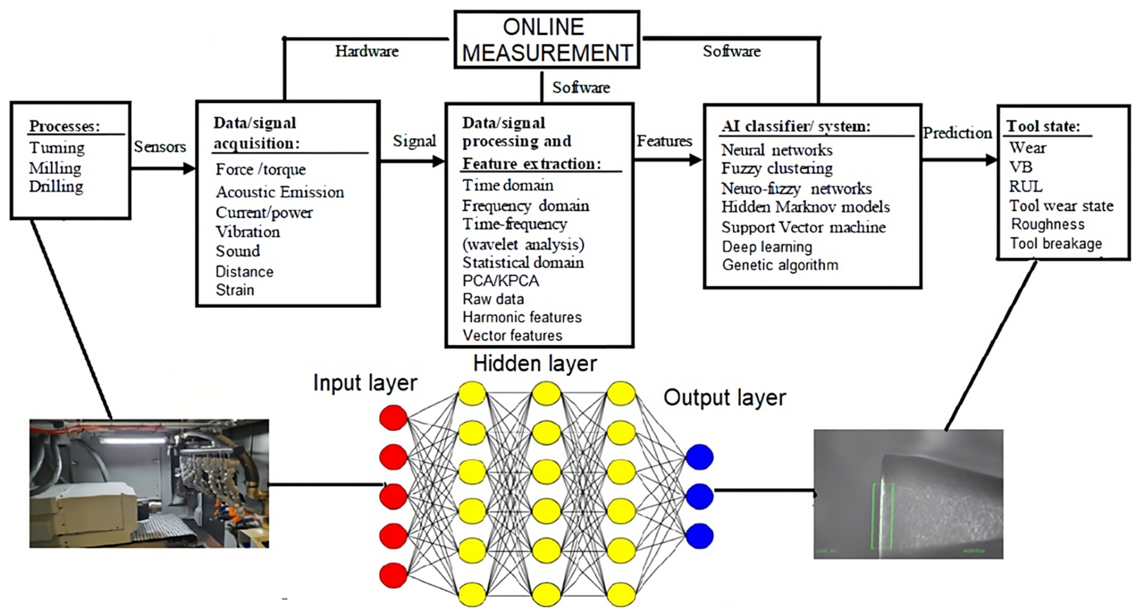
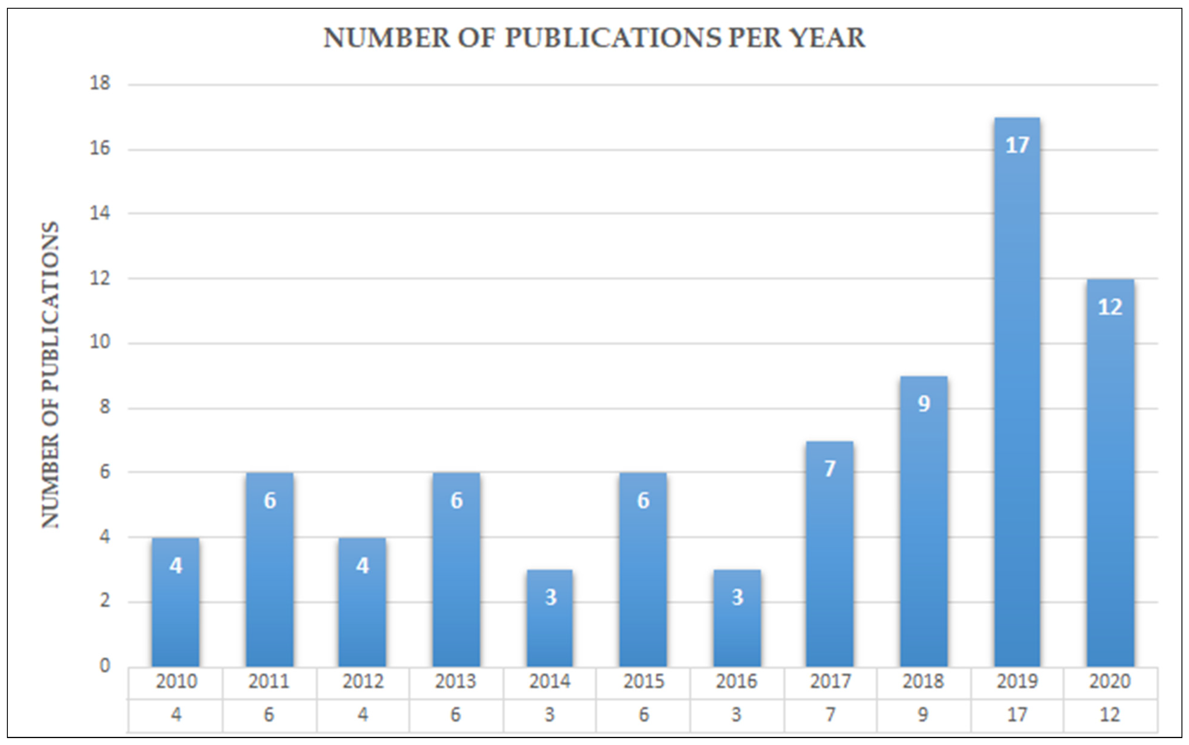
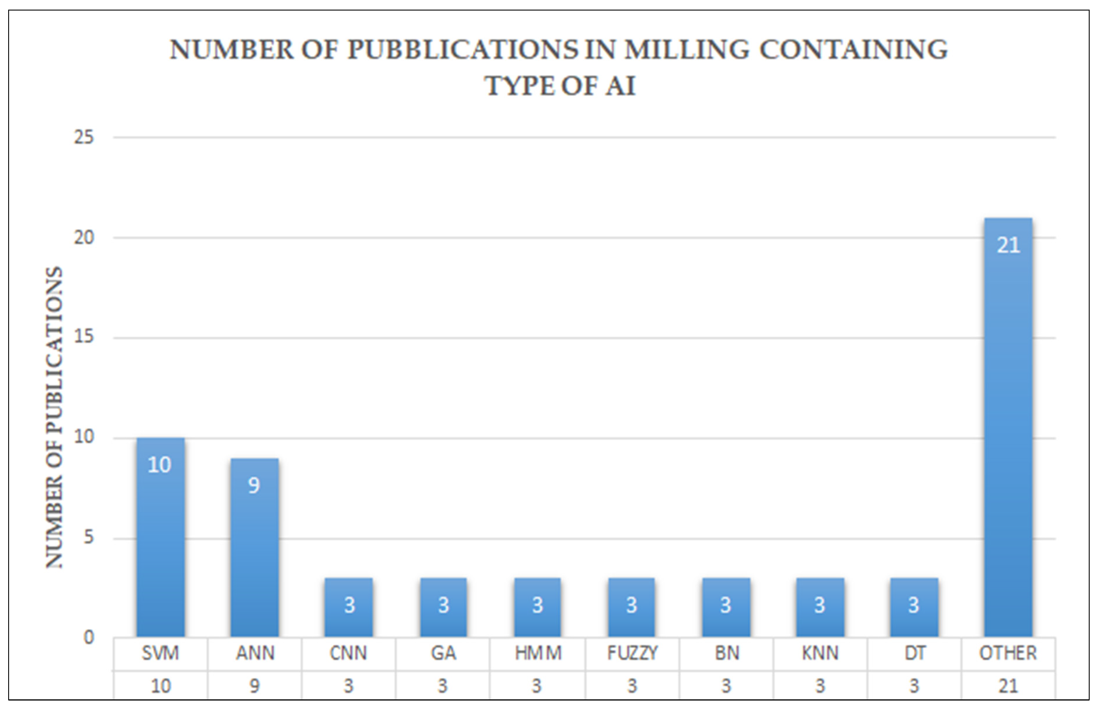
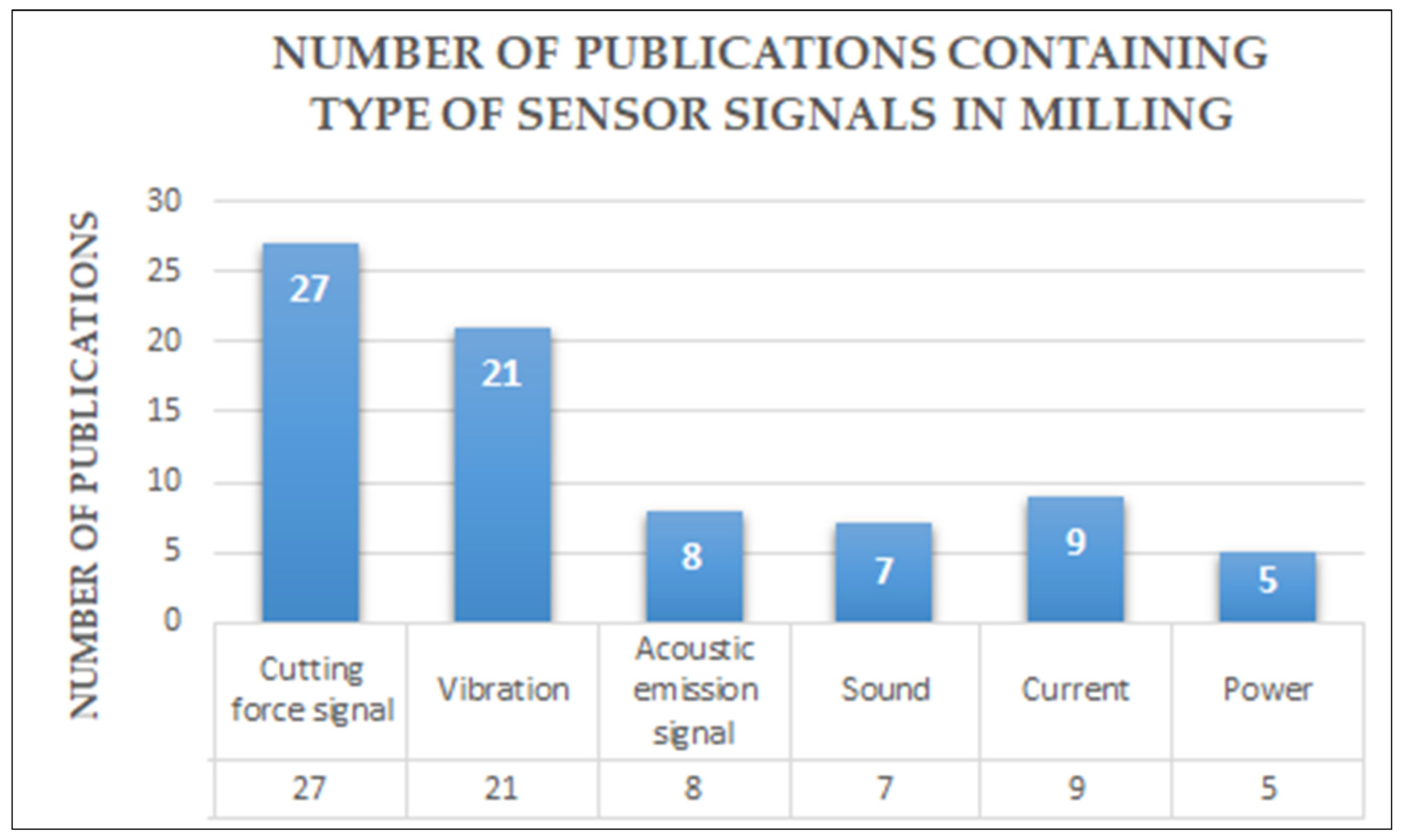
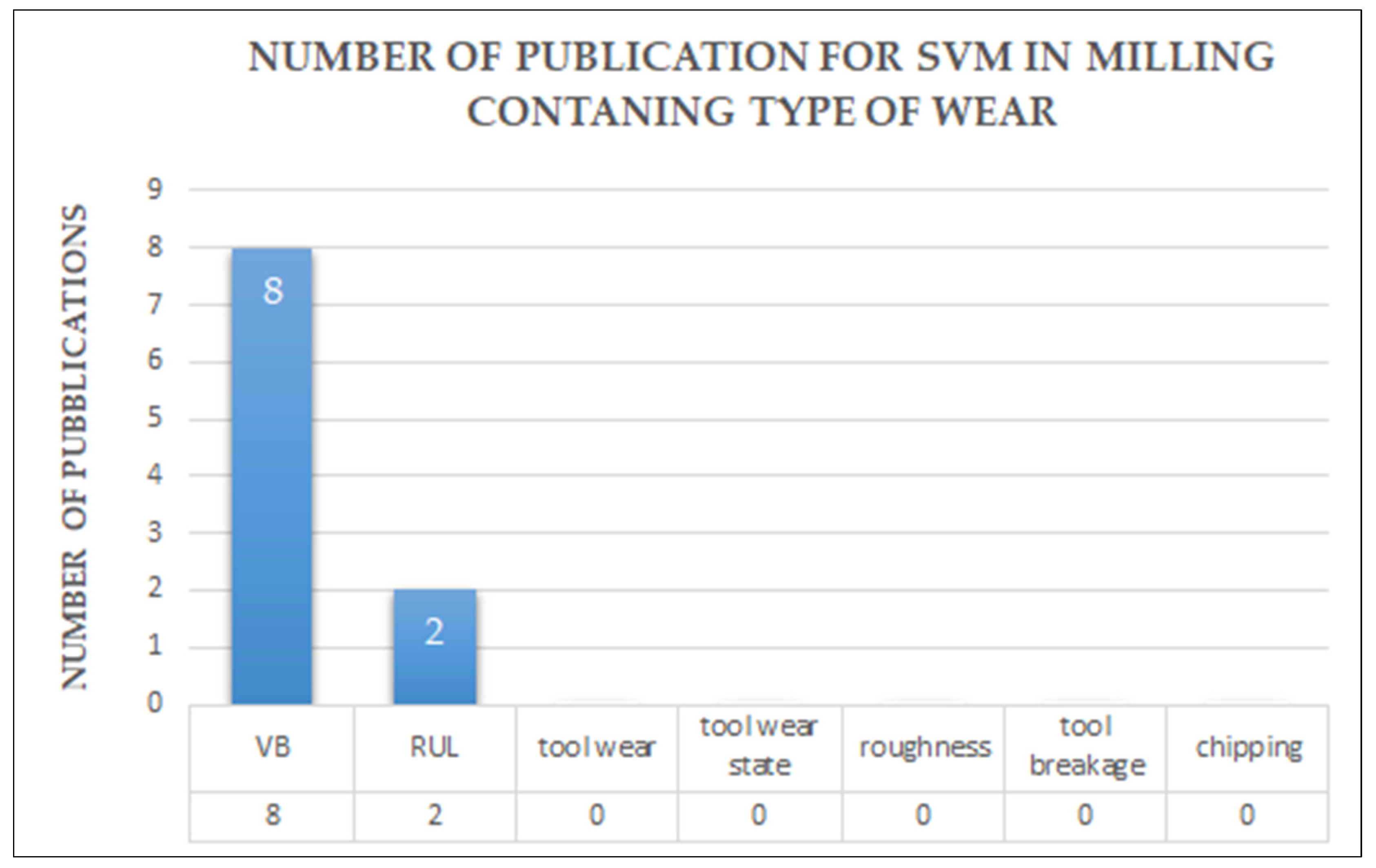
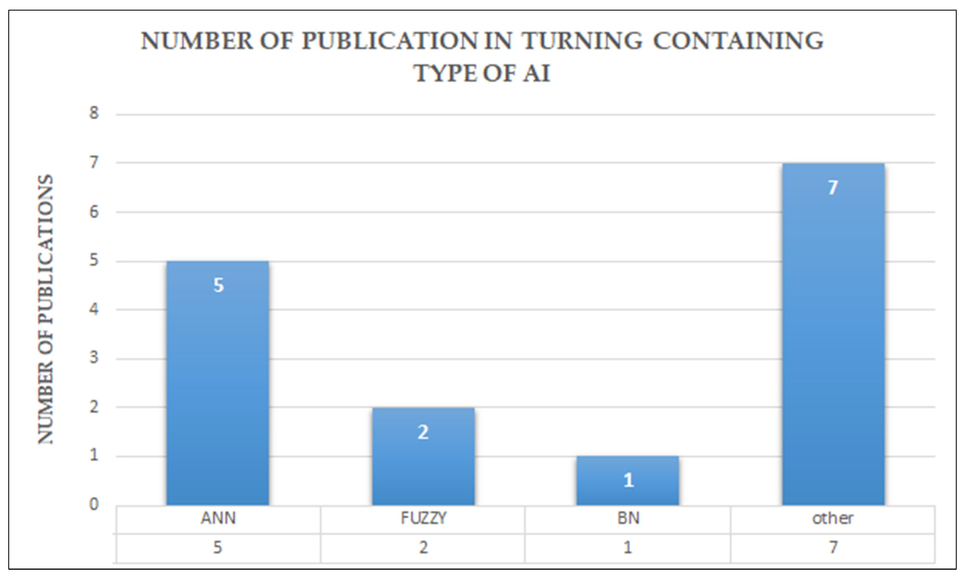
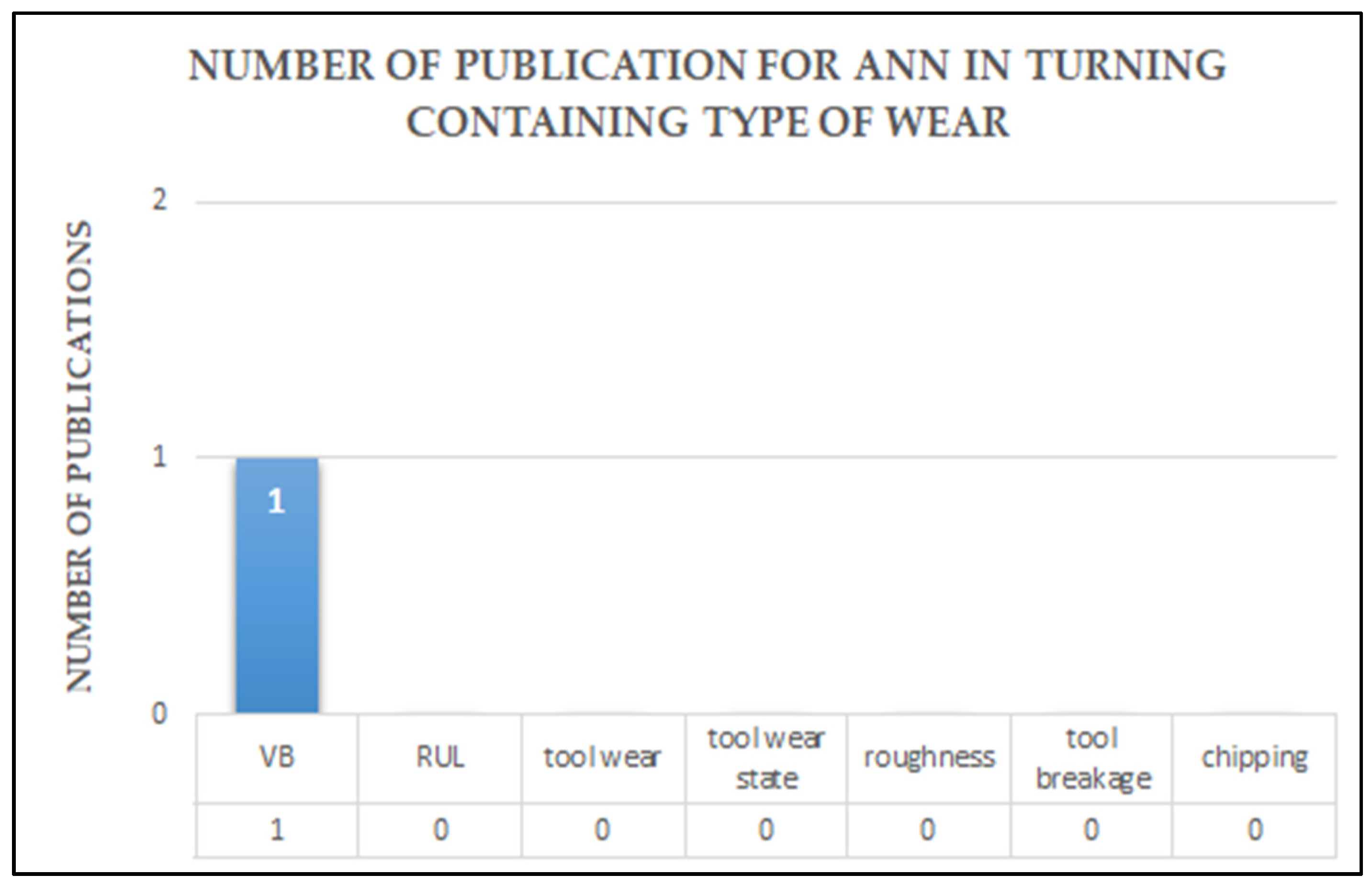
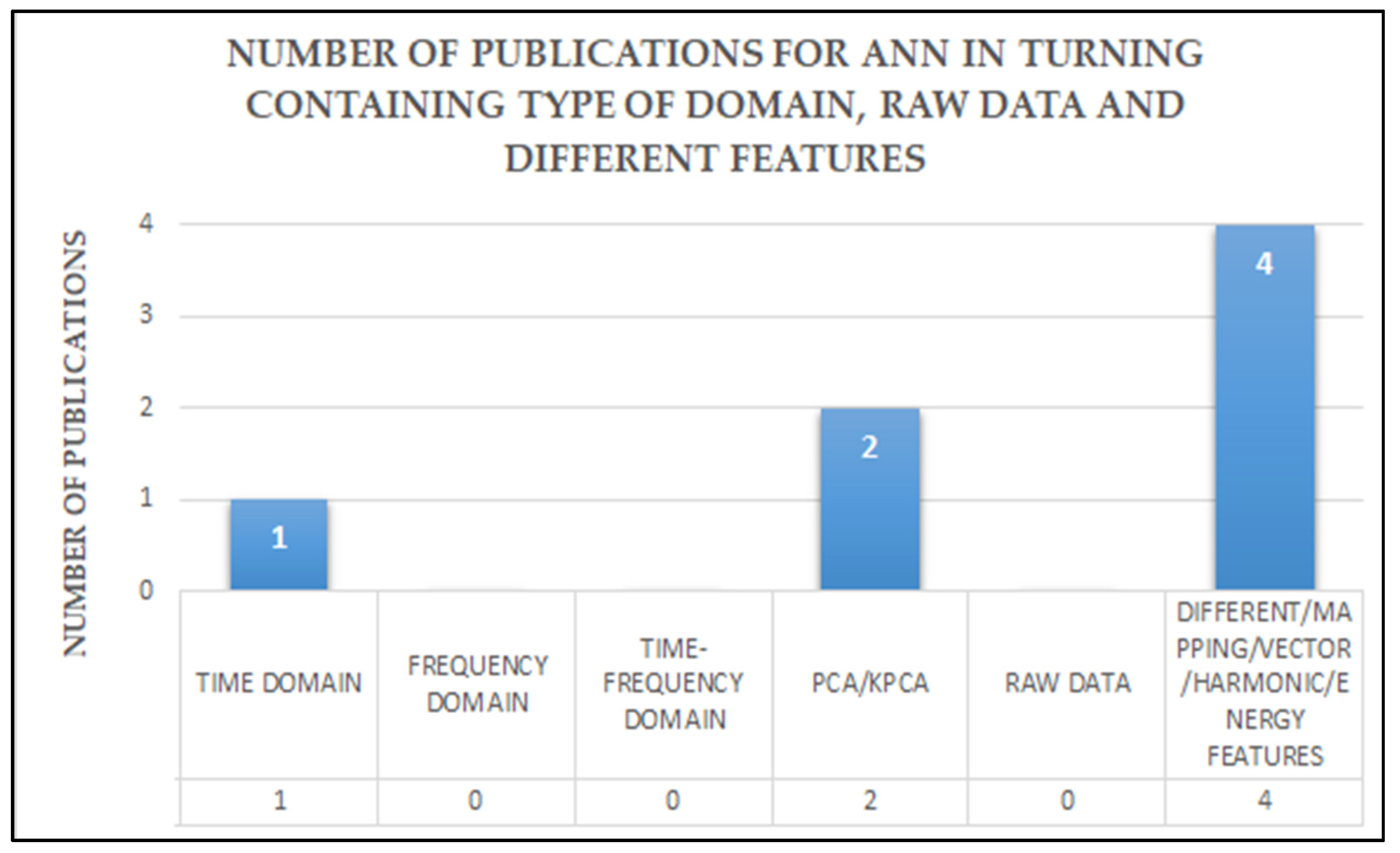
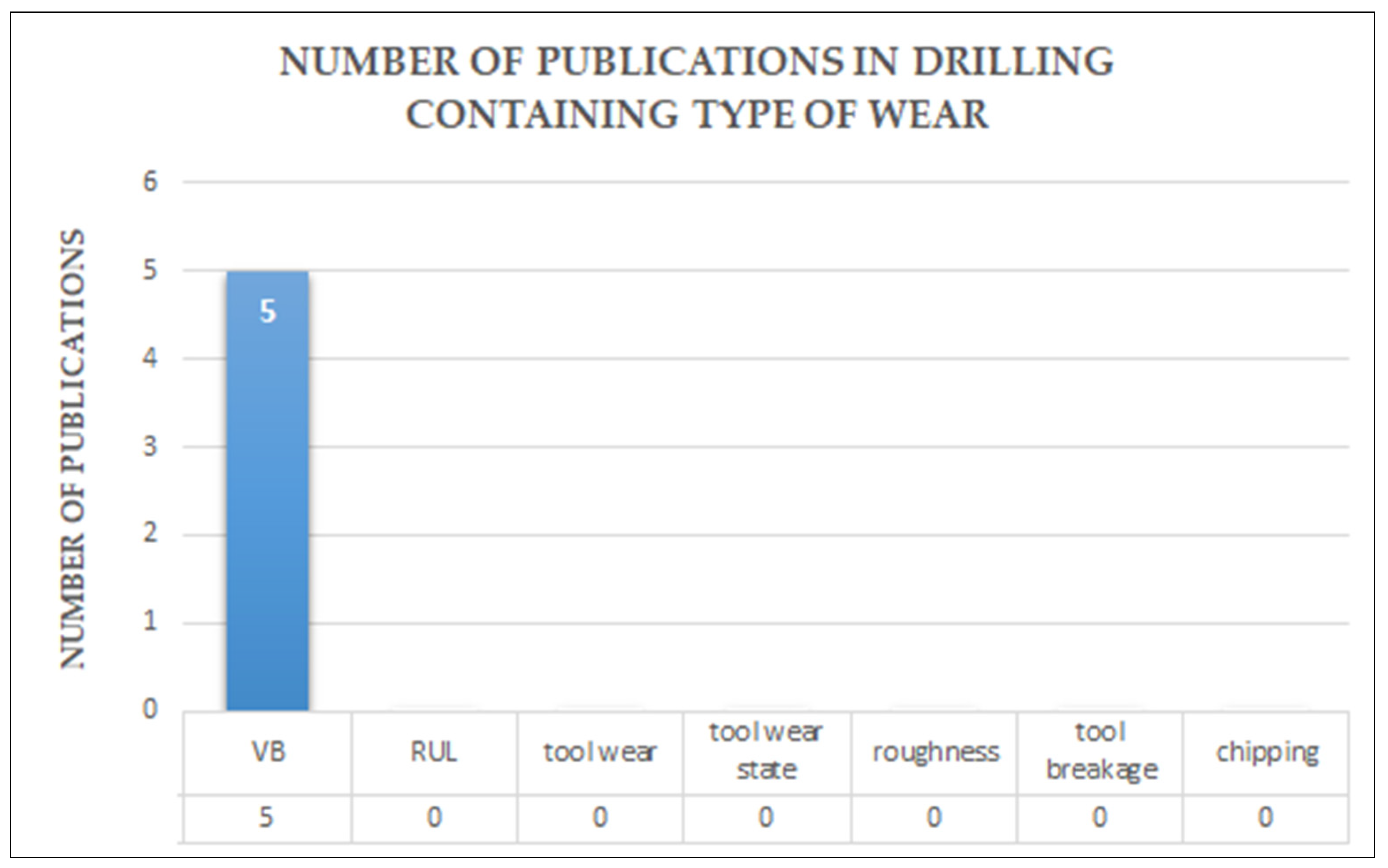
Table A1.
Checklist review.
| Abstract | ||
| Introduction | 1 | |
| Objectives | Provide an answer to your research | |
| Research Question | Provide an explicit statement of the question(s) the review will address | |
| Methods Of Research Level, Research’s Item And Research’s Number Of Published Articles Found | 2 | |
| Eligibility Criteria Search Strategy | 2.1 | Specify the study characteristics (study design, setting, time frame) and report characteristics (such as years considered, language, publication status) to be used as criteria for eligibility for the review. Present draft of search strategy to be used for at least one electronic database, including planned limits, such that it could be repeated |
| Selection Of Offline And Online Publications And Related Data Extraction From The Publications | 3 | |
| Results Of Research | 4 | |
| Introduction Selection and Inclusion of Publications | 4.1 | It describes which articles were included |
| General And Essential Requirement Of Machining Operations, Number Of Articles, Type Of Wear, Type Of Machine And Type Of Material | 4.2 | It describes the essential and general requirements of the articles identified and selected |
| Introduction Methods of Measurement | 4.3 | Describes in general the online and offline measurement systems. 4.3.1 Offline measurement 4.3.2 Measurement online |
| Type of Sensors and How They are used in research Experiments | 4.4 | Describes the signal that the dedicated sensor detects. 4.4.1 Cutting Force sensors 4.4.2 Vibration sensors 4.4.3 AE Emission Acoustic sensors 4.4.4 Sound sensors 4.4.5 Current and power sensors |
| Features Of Signal, AI Methods And Performances | 4.5 | It describes the features extracted from the signals, the AI methods to predict the tool wear and the performances of the algorithms. 4.5.1 Introduction of Features Sensor Signal 4.5.2 Features sensor signal in different domani: Time domain—Frequency domain—Time Frequency domain—Other 4.5.3 Introduction and General Explanation of AI methods Methods of AI applications: ANN, GA, FL, SVM, HMM, DT, RF, ANFIS, BN, KNN, PCA, CNN, C-mean, RVM, ELM, SSA, KALMN FILTER, CRF AI applications in milling. Analyse SVM in milling. AI applications in turning Analysis ANN in turning AI applications in drilling 4.5.4 Performances 4.5.4 Introduction of the Performance of an AI algorithm Performance of an AI algorithm in milling, turning and drilling |
| Industrial Application And Future Trends Of Research | 5 | |
| Results And Conclusion Compared With Recent Reviews | 6 | 6.1 Result review 6.2 Conclusions compared with recent reviews |
Appendix B
Table A2.
Features, signal, AI methods and performances in milling.
| Domain | |||||||
|---|---|---|---|---|---|---|---|
| Articles | Time | Frequency | Time-Frequency | Pca/Kpca | Signal | A.I. Methods | Performance |
| [8] | x | x | x | Cutting force, power and current | FCNN with MAML | Prediction error | |
| [10] | x | Sound | CNN with SGD | Predictive accuracy | |||
| [11] | x | x | Current | SVM, LDA; KNN, NN, NB, DT | Accuaracy. | ||
| [12] | different feature | Cutting force, vibration and acoustic emission | HMM | MAPE, Mean and Accuracy | |||
| [13] | x | x | Sound | CART, RF, KNN, SVM with EBCA and without EBCA | accuracy with training set 50–60–70–80% | ||
| [14] | x | x | Cutting force | RVM, SVM | Accuracy | ||
| [15] | x | x | Cutting force | dGAM | k-fold cross and accuracy | ||
| [16] | statistical feature | Cutting force | ANN | R, MRE, R² | |||
| [17] | x | x | Cutting force,vibration | FCM | FBE | ||
| [19] | x | x | x | Cutting force,vibration | EAM ARTMAP, FUZZY ARTMAP (FAM) | averaging recognition rate | |
| [20] | images for force | Cutting force | CNN, AC | Predicted Rapid initial wear, Predicted Uniform wear, Predicted Failure wear Accuracy % | |||
| [22] | different feature | Cutting force, vibration and acoustic emission | SSAE | Average accuracy | |||
| [25] | x | x | x | Cutting force, vibration | PGGM | RMSE, MAE | |
| [27] | x | x | x | x | Cutting force | RVM with KPCA-IRBF | RMSE, PCC, CI_widht/CI_var |
| [32] | raw data | Cutting force | CNN+BILSTM and CNN+BIGRU | MAE, RMSE | |||
| [33] | x | Vibration | ANN, SVM and KNN | Score, recall and precision | |||
| [34] | different feature | Cutting force | Kalman filter | RMSE | |||
| [35] | different feature | Acoustic emission | CRF and HMM | accuracy rate | |||
| [37] | x | Power | R² | ||||
| [38] | feature mapping | x | Power and current | BP | formula tool life predicting | ||
| [39] | x | x | x | Cutting force, current | SVM, RF and feedforrward NN | Score, RMSE and Accuracy | |
| [41] | x | x | Vibration, acoustic emission, current | DBILSTM | MAE and RMSE | ||
| [42] | x | x | Cutting force, vibration and sound | TAKELM, BDE | MAE, MAPE, RMSE | ||
| [44] | x | Sound | GAN | accuracy, non-confroming tool | |||
| [45] | x | Vibration | K-star | positive rate (TP rate) and false positive rate (FP rate) and accuracy | |||
| [46] | x | Sound | DCNN | accuracy | |||
| [47] | x | x | x | Cutting force, vibration | SVR, CNN, LSTM, GRU | RMSE and MAE | |
| [48] | feature vector | Sound | HMM | SR | |||
| [50] | x | x | x | x | Cutting force, vibration | PF, AR-PF, SVR-PF | RMSE |
| [52] | images feature | Power | NN inconrporate CNN and RNN NN incorporate RNN | accuracy | |||
| [53] | harmonic feature | Cutting force | ARTMAP (GAM) | accuracy | |||
| [54] | raw data | Power | Kalman filter | RMSE, average percent error | |||
| [56] | x | x | Vibration and emission acoustic | LR, DF, BLR, DT, NN | RMSE, RelSE and R² | ||
| [57] | x | x | Vibration, emission acoustic and sound | BP, SVM, ANFIS | RMSE, COV and R² | ||
| [58] | x | x | x | x | Cutting force, vibration | KPCA, LLE, ISOMAP, mRMR | RMSE, PCC, MAE and MAPE |
| [60] | Feature based fusion | Cutting force | VARX-L, SVR, RF, XGBOOST | NRMSE | |||
| [61] | x | x | x | Cutting force | DE-SVR | Accuracy VB and Acccuracy RUL | |
| [62] | raw data | Sound | SVM | maximum shape error | |||
| [63] | x | x | Vibration | SVM with TIPM SVM without TIPM | accuracy | ||
| [64] | holder exponent feature | Vibration | SVM | RMSE and accuracy | |||
| [65] | raw data | Specific Cutting Forces | DNN, LR | R² and RMSE | |||
| [71] | force and vibration feature | Cutting force, vibration | ELM, SW-ELM, ESN | R² | |||
| [72] | x | x | Cutting force | NB | R² | ||
| [73] | DWT features, EMD features, statistical features | Sound | SVM, ANN, NB, K-star | true positive rate (TP rate) false positive rate (FP rate) | |||
| [74] | energy feature vector | Cutting force, current | CHMM | accuracy | |||
| [75] | raw data | Vibration and current | R² | ||||
| [76] | x | x | x | Vibration | NFN, BP, RBFN | MSE, MAPE and R² | |
| [77] | harmonic feature | Cutting force | ARTMAP | Incremental learning | |||
| [78] | raw data | Cutting force, vibration and emission acoustic | HMM | MSE, accuracy | |||
| [81] | x | x | x | Cutting force, vibration and emission acoustic | GA with KELM | R², RMSE | |
Appendix C
Table A3.
Features, signal, AI methods and performances in turning.
| DOMAIN | |||||||
|---|---|---|---|---|---|---|---|
| Articles | Time | Frequency | Time-Frequency | Pca/Kpca | Signal | Neural Network | Performance |
| [18] | x | x | x | x | Cutting force | KPCA_IRBF | GPR model, MAE, RMSE, MAPE, PCC, CI |
| [21] | feature vector | Cutting force, torque, vibration acoustic emission | NN | SR | |||
| [23] | x | x | Vibration signal | TBTCD, FCM Classifier, Lasso classifier | recognition accuracy | ||
| [24] | x | Cutting force, vibration | ANFIS algorithm | MAPE | |||
| [26] | x | x | Cutting force, vibration | GUI | Different between measured wear and calculated wear | ||
| [28] | feature vector | x | Cutting force, vibration and acoustic emission | NN with PCA | SR | ||
| [30] | statistical feature | Vibration | K-star | TP rate’ and ‘FP rate define the accuracy | |||
| [31] | raw data | Acoustic emission | TSK | RMSE | |||
| [36] | different feature | Cutting force | TSK, NN, Mandami FL, NF | RMSE and MAX | |||
| [40] | x | x | x | Vibration and power | FBNF | R² and RMSE | |
| [59] | Sensorial features, feature pattern vector. | x | Cutting force, vibration and emission acoustic | NN, FFBP | Consumed tool life% average error % | ||
| [68] | x | Vibration and emission acoustic | ANN | Accuracy | |||
| [70] | raw data | Cuttin force and emission acoustic | DENFIS, TWNFIS, ANFIS | SSE, NSSE, FPE, ENV, SBC, TAE and average error | |||
| [79] | x | Vibration, emission acoustic and current | proportional hazard model | logarithmic means and logarithmic standard deviations | |||
| [80] | x | x | x | Cutting force, vibration and emission acoustic | Decision-making algorithm | R², RMSE | |
Appendix D
Table A4.
Features, signal, AI methods and performances in drilling.
| DOMAIN | |||||||
|---|---|---|---|---|---|---|---|
| Articles | Time | Frequency | Time-Frequency | Pca/Kpca | Signal | Neural Network | Performance |
| [9] | x | Cutting force, acoustic emission | K-means | Sum Squared Error | |||
| [29] | different feature | Cutting force and power | LM, CGD and BI | MSE and the R² | |||
| [43] | raw data | Current and power | RF | accuracy, R², MAE,RMSE | |||
| [49] | x | Vibration | K-star | accuracy | |||
| [51] | raw data | Cutting force | RBFN with GA | MSE and % MSE | |||
References
- Zhang, C.; Zhang, J. On-line tool wear measurement for ball-end milling cutter based on machine vision. Comput. Ind. 2013, 64, 708–719. [Google Scholar] [CrossRef]
- Barreiro, J.; Fernández-Abia, A.; González-Laguna, A.; Pereira, O. TCM system in contour milling of very thick very large steel plates based on vibration and AE signal. J. Mater. Process. Technol. 2017, 246, 144–157. [Google Scholar] [CrossRef]
- Rehorn, A.; Jiang, J.; Orban, P.; Bordatchev, E. State-of-the-art methods and results in tool condition monitoring: A review. Int. J. Adv. Manuf. Technol. 2004, 26, 942. [Google Scholar] [CrossRef] [Green Version]
- Dimla, D. Sensor signals for tool wear monitoring in metal cutting operations a review of methods. Int. J. Mach. Tool. Manuf. 2000, 40, 1073–1098. [Google Scholar] [CrossRef]
- Zhang, X.Y.; Lu, X.; Wang, S.; Wang, W.; Li, W.D. A multi-sensor based online tool condition monitoring system for milling process. Procedia CIRP 2018, 72, 1136–1141. [Google Scholar] [CrossRef]
- Shamseer, L.; Moher, D.; Clarke, M.; Ghersi, D.; Liberati, A.; Petticrew, M.; Shekelle, P.; Stewart, L. Preferred reporting items for systematic review and meta-analysis protocols (PRISMA-P): Elaboration and explanation. BMJ 2015, 349, g7647. [Google Scholar] [CrossRef] [PubMed] [Green Version]
- ISO 1832:2012; Indexable Inserts for Cutting Tools—Designation. ISO: Geneva, Switzerland. Available online: https://standards.iteh.ai/catalog/standards/iso/1777acf9-65d1-40f2-ac15-02b7c1ead78a/iso-1832-2004 (accessed on 23 July 2011).
- Li, Y.; Liu, C.; Hua, J.; Gao, J.; Maropoulos, P. A novel method for accurately monitoring and predicting tool wear under varying cutting conditions based on meta-learning. CIRP Ann. 2019, 68, 487–490. [Google Scholar] [CrossRef]
- Klocke, F.; Döbbeler, B.; Pullen, T.; Bergs, T. Acoustic emission signal source separation for a flank wear estimation of drilling tools. Procedia CIRP 2019, 79, 57–62. [Google Scholar] [CrossRef]
- Kothuru, A.; Nooka, S.P.; Liu, R. Application of deep visualization in CNN-based tool condition monitoring for end milling. Procedia Manuf. 2019, 34, 995–1004. [Google Scholar] [CrossRef]
- Hassan, M.; Damir, A.; Attia, H.; Thomson, V. Benchmarking of Pattern Recognition Techniques for Online Tool Wear Detection. Procedia CIRP 2018, 72, 1451–1456. [Google Scholar] [CrossRef]
- Tobon-Mejia, D.A.; Medjaher, B.K.; Zerhouni, N. CNC machine tool’s wear diagnostic and prognostic by using dynamic Bayesian networks. Mech. Syst. Signal Process. 2012, 28, 167–182. [Google Scholar] [CrossRef] [Green Version]
- Li, Z.; Liu, R.; Wu, D. Data-driven smart manufacturing: Tool wear monitoring with audio signals and machine learning. J. Manuf. Process. 2019, 48, 66–76. [Google Scholar] [CrossRef]
- Wang, G.; Yang, Y.; Xie, Q.; Zhang, Y. Force based tool wear monitoring system for milling process based on relevance vector machine. Adv. Eng. Softw. 2014, 71, 46–51. [Google Scholar] [CrossRef]
- Wang, G.; Guo, Z.; Yang, Y. Force sensor based online tool wear monitoring using distributed Gaussian ARTMAP network. Sens. Actuators A Phys. 2013, 192, 111–118. [Google Scholar] [CrossRef]
- Kaya, B.; Oysu, C.; Ertunc, H.M. Force-torque based on-line tool wear estimation system for CNC millingof Inconel 718 using neural networks. Adv. Eng. Softw. 2011, 42, 76–84. [Google Scholar] [CrossRef]
- Fua, P.; Li, W.; Guo, L. Fuzzy Clustering and Visualization Analysis of Tool Wear Status Recognition. Procedia Eng. 2011, 23, 479–486. [Google Scholar] [CrossRef]
- Kong, D.; Chen, Y.; Li, N. Gaussian process regression for tool wear prediction. Mech. Syst. Signal Process. 2018, 104, 556–574. [Google Scholar] [CrossRef]
- Liu, C.; Wang, G.F.; Li, Z.M. Incremental learning for online tool condition monitoring using Ellipsoid ARTMAP network model. Appl. Soft Comput. 2015, 35, 186–198. [Google Scholar] [CrossRef]
- Gouarir, A.; Martinez-Arellano, G.; Terrazas, G.; Benardos, P.; Ratchev, S. In process tool wear prediction system based on machine learning techniques and force analysis. Procedia CIRP 2018, 77, 501–504. [Google Scholar] [CrossRef]
- Segreto, T.; Simeone, A.; Teti, R. Multiple sensor monitoring in nickel alloy turning for tool wear assessment via sensor fusion. Procedia CIRP 2013, 12, 85–90. [Google Scholar] [CrossRef]
- Ochoa, L.E.E.; Quinde, I.B.R.; Sumba, J.P.C.; Guevara, A.J.V.; Menendez, R.M. New Approach based on Autoencoders to Monitor the Tool Wear Conditionin HSM. IFAC-PapersOnLine 2019, 52, 206–211. [Google Scholar] [CrossRef]
- Antic, A.; Popovic, B.; Krstanovic, L.; Obradovic, R.; Miloševic, M. Novel texture-based descriptors for tool wear condition monitoring. Mech. Syst. Signal Process. 2018, 98, 1–15. [Google Scholar] [CrossRef]
- Rizal, M.; Ghani, J.A.; Nuawi, M.Z.; Haron, C.H.C. Online tool wear prediction system in the turning process using an adaptive neuro-fuzzy inference system. Appl. Soft Comput. 2013, 13, 1960–1968. [Google Scholar] [CrossRef]
- Wang, J.; Li, Y.; Zhao, R.; Gao, R.X. Physics guided neural network for machining tool wear prediction. J. Manuf. Syst. 2020, 57, 298–310. [Google Scholar] [CrossRef]
- Mali, R.; Telsang, M.T.; Gupta, T.V.K. Real Time Tool Wear Condition Monitoring in Hard Turning of Inconel 718 Using Sensor Fusion System. Mater. Today Proc. 2017, 4, 8605–8612. [Google Scholar] [CrossRef]
- Kong, D.; Chen, Y.; Li, N.; Duan, C.; Lu, L.; Chen, D. Relevance vector machine for tool wear prediction. Mech. Syst. Signal Process. 2019, 127, 573–594. [Google Scholar] [CrossRef]
- Segreto, T.; Simeone, A.; Teti, R. Sensor Fusion for Tool State Classification in Nickel Superalloy High Performance Cutting. Procedia CIRP 2012, 1, 593–598. [Google Scholar] [CrossRef]
- Corne, R.; Nath, C.; El Mansori, M.; Kurfess, T. Study of spindle power data with neural network for predictingreal-time tool wear/breakage during inconel drilling. J. Manuf. Syst. 2017, 43, 287–295. [Google Scholar] [CrossRef]
- Painuli, S.; Elangovan, M.; Sugumaran, V. Tool condition monitoring using K-star algorithm. Expert. Syst. Appl. 2014, 41, 2638–2643. [Google Scholar] [CrossRef]
- Ren, Q.; Baron, L.; Balazinski, M.; Botez, R.; Bigras, P. Tool wear assessment based on type-2 fuzzy uncertainty estimation on acoustic emission. Appl. Soft Comput. 2015, 31, 14–24. [Google Scholar] [CrossRef]
- Ma, J.; Luo, D.; Liao, X.; Zhang, Z.; Huang, Y.; Lu, J. Tool wear mechanism and prediction in milling TC18 titanium alloy using deep learning. Measurement 2021, 173, 108554. [Google Scholar] [CrossRef]
- Hesser, D.F.; Markert, B. Tool wear monitoring of a retrofitted CNC milling machine using artificial neural networks. Manuf. Lett. 2019, 19, 1–4. [Google Scholar] [CrossRef]
- Tiwari, K.; Shaik, A.; Arunachalam, N. Tool wear prediction in end milling of Ti-6Al-4V through Kalman filter based fusion of texture features and cutting forces. Procedia Manuf. 2018, 26, 1459–1470. [Google Scholar] [CrossRef]
- Wangn, G.; Feng, X. Tool wear state recognition based on linear chain conditional random field model. Eng. Appl. Artif. Intell. 2013, 26, 1421–1427. [Google Scholar] [CrossRef]
- Ren, Q.; Balazinski, M.; Baron, L.; Jemielniak, K. TSK fuzzy modeling for tool wear condition in turning processes: An experimental study. Eng. Appl. Artif. Intell. 2011, 24, 260–265. [Google Scholar] [CrossRef]
- Goodall, P.; Pantazis, D.; West, A. A cyber physical system for tool condition monitoring using electrical power and a mechanistic model. Comput. Ind. 2020, 118, 103223. [Google Scholar] [CrossRef]
- Bao, J.; Yuan, G.; Zheng, X.; Zhang, J.; Xia, J. A Data Driven Model for Predicting Tool Health Condition in High Speed Milling of Titanium Plates Using Real-Time SCADA. Procedia CIRP 2017, 61, 317–322. [Google Scholar] [CrossRef]
- An, Q.; Tao, Z.; Xu, X.; El Mansori, M.; Chen, M. A data-driven model for milling tool remaining useful life prediction with convolutional and stacked LSTM network. Measurement 2020, 154, 107461. [Google Scholar] [CrossRef]
- Zhang, B.; Shin, Y.C. A multimodal intelligent monitoring system for turning processes. J. Manuf. Process. 2018, 35, 547–558. [Google Scholar] [CrossRef]
- Li, H.; Wang, W.; Li, Z.; Dong, L.; Li, Q. A novel approach for predicting tool remaining useful life using limited data. Mech. Syst. Signal Process. 2020, 143, 106832. [Google Scholar] [CrossRef]
- Zhou, Y.; Sun, B.; Sun, W. A tool condition monitoring method based on two-layer angle kernelextreme learning machine and binary differential evolution for milling. Measurement 2020, 166, 108186. [Google Scholar] [CrossRef]
- Oberlè, R.; Schorr, S.; Yi, L.; Glatt, M.; BaHre, D.; Aurich, J.C. A Use Case to Implement Machine Learning for Life Time Prediction of Manufacturing tools. Procedia CIRP 2020, 93, 1484–1489. [Google Scholar] [CrossRef]
- Cooper, C.; Zhang, J.; Gao, R.X.; Wang, P.; Ragai, I. Anomaly detection in milling tools using acoustic signals and generative adversarial networks. Procedia Manuf. 2020, 48, 372–378. [Google Scholar] [CrossRef]
- Madhusudana, C.K.; Kumar, H.; Narendranath, S. Condition monitoring of face milling tool using K-star algorithm and histogram features of vibration signal. Eng. Sci. Technol. Int. J. 2016, 19, 1543–1551. [Google Scholar] [CrossRef] [Green Version]
- Cooper, C.; Wang, P.; Zhang, J.; Gao, R.X.; Roney, T.; Ragai, I.; Shaffer, D. Convolutional neural network-based tool condition monitoring in vertical milling operations using acoustic signals. Procedia Manuf. 2020, 49, 105–111. [Google Scholar] [CrossRef]
- Wang, J.; Yan, J.; Li, C.; Gao, R.X.; Zhao, R. Deep heterogeneous GRU model for predictive analytics in smart manufacturing: Application to tool wear prediction. Comput. Ind. 2019, 111, 1–14. [Google Scholar] [CrossRef]
- Boutros, T.; Liang, M. Detection and diagnosis of bearing and cutting tool faults using hidden Markov models. Mech. Syst. Signal Process. 2011, 25, 2102–2124. [Google Scholar] [CrossRef]
- Simon, G.D.; Deivanathan, R. Early detection of drilling tool wear by vibration data acquisition and classification. Manuf. Lett. 2019, 21, 60–65. [Google Scholar] [CrossRef]
- Wanga, J.; Wang, P.; Gao, R.X. Enhanced particle filter for tool wear prediction. J. Manuf. Syst. 2015, 36, 35–45. [Google Scholar] [CrossRef]
- Garg, S.; Patra, K.; Khetrapal, V.; Pal, S.K.; Chakraborty, D. Genetically evolved radial basis function network based prediction of drill flank wear. Eng. Appl. Artif. Intell. 2010, 23, 1112–1120. [Google Scholar] [CrossRef]
- Wang, P.; Liu, Z.; Gao, R.X.; Guo, Y. Heterogeneous data-driven hybrid machine learning for tool condition prognosis. CIRP Ann. 2019, 68, 455–458. [Google Scholar] [CrossRef]
- Wang, G.; Yang, Y.; Guo, Z. Hybrid learning based Gaussian ARTMAP network for tool conditionmonitoring using selected force harmonic features. Sens. Actuators A Phys. 2013, 203, 394–404. [Google Scholar] [CrossRef]
- Niaki, F.A.; Ulutan, D.; Mears, L. In-Process Tool Flank Wear Estimation in Machining Gamma-Prime Strengthened Alloys Using Kalman Filter. Procedia Manuf. 2015, 1, 696–707. [Google Scholar] [CrossRef] [Green Version]
- Nath, C. Integrated Tool Condition Monitoring Systems and Their Applications: A Comprehensive Review. Procedia Manuf. 2020, 48, 852–863. [Google Scholar] [CrossRef]
- Traini, E.; Bruno, G.; D’Antonio, G.; Lombardi, F. Machine Learning Framework for Predictive Maintenance in Milling. IFAC-PapersOnLine 2019, 52, 177–182. [Google Scholar] [CrossRef]
- Wu, J.; Su, Y.; Cheng, Y.; Shao, X.; Deng, C.; Liu, C. Multi-sensor information fusion for remaining useful life prediction of machining tools by adaptive network based fuzzy inference system. Appl. Soft Comput. 2018, 68, 13–23. [Google Scholar] [CrossRef]
- Wang, J.; Xie, J.; Zhao, R.; Zhang, L.; Duan, L. Multisensory fusion based virtual tool wear sensing for ubiquitous manufacturing. Robot. Comput. Int. Manuf. 2017, 45, 47–58. [Google Scholar] [CrossRef] [Green Version]
- Karam, S.; Centobelli, P.; D’Addona, D.M.; Teti, R. Online prediction of cutting tool life in turning via cognitive decision making. Procedia CIRP 2016, 41, 927–932. [Google Scholar] [CrossRef]
- Finkeldey, F.; Saadallah, A.; Wiederkehr, P.; Morik, K. Real-time prediction of process forces in milling operations using synchronized data fusion of simulation and sensor data. Eng. Appl. Artif. Intell. 2020, 94, 103753. [Google Scholar] [CrossRef]
- Yang, Y.; Guo, Y.; Huang, Z.; Chen, N.; Li, L.; Jiang, Y.; He, N. Research on the milling tool wear and life prediction by establishing an integrated predictive model. Measurement 2019, 145, 178–189. [Google Scholar] [CrossRef]
- Denkena, B.; Dittrich, M.A.; Mainka, J. Simulation-based feed rate adaptation considering tool wear condition. Procedia Manuf. 2020, 52, 133–137. [Google Scholar] [CrossRef]
- Wang, G.F.; Yang, Y.W.; Zhang, Y.C.; Xie, Q.L. Vibration sensor based tool condition monitoring using supportvector machine and locality preserving projection. Sens. Actuators A Phys. 2014, 209, 24–32. [Google Scholar] [CrossRef]
- Zhou, C.; Yang, B.; Guo, K.; Liu, J.; Sun, J.; Song, G.; Zhu, S.; Sun, C.; Jiang, Z. Vibration singularity analysis for milling tool condition monitoring. Int. J. Mech. Sci. 2020, 166, 105254. [Google Scholar] [CrossRef]
- Peng, B.; Bergs, T.; Schraknepper, D.; Klocke, F.; Döbbeler, B. A hybrid approach using machine learning to predict the cutting forces under consideration of the tool wear. Procedia CIRP 2019, 82, 302–307. [Google Scholar] [CrossRef]
- Siddhpura, A.; Paurobally, R. A review of flank wear prediction methods for tool condition monitoring in a turning process. Int. J. Adv. Manuf. Technol. 2013, 65, 371–393. [Google Scholar] [CrossRef]
- Zhou, Y.; Xue, W. Review of tool condition monitoring methods in milling processes. Int. J. Adv. Manuf. Technol. 2018, 96, 2509–2523. [Google Scholar] [CrossRef]
- Lee, S.S. Tool condition monitoring system in turning operation utilizing wavelet signal processiing and multi-learning ANNs algorithm methodology. Int. J. Eng. Res. Innov. 2010, 2, 49. [Google Scholar]
- Downey, J.; O’Sullivan, D.; Nejmen, M.; Bombinski, S.; O’Leary, P.; Raghavendra, R.; Jemielniak, K. Real time monitoring of the CNC process in a production environment the data collection & analysis phase. Procedia CIRP 2016, 41, 920–926. [Google Scholar] [CrossRef] [Green Version]
- Gajate, A.; Haber, R.; Del Toro, R.; Vega, P.; Bustillo, A. Tool wear monitoring using neuro-fuzzy techniques: A comparative study in a turning process. J. Intell. Manuf. 2012, 23, 869–882. [Google Scholar] [CrossRef] [Green Version]
- Karandikar, J.; McLeay, T.; Turner, S.; Schmitz, T. Tool wear monitoring and prognostics challenges: A comparison of connectionist methods toward an adaptive ensemble model. J. Intell. Manuf. 2018, 29, 1873–1890. [Google Scholar] [CrossRef]
- Karandikar, J.; McLeay, T.; Turner, S.; Schmitz, T. Tool wear monitoring using naïve Bayes classifiers. Int. J. Adv. Manuf. Technol. 2015, 77, 1613–1626. [Google Scholar] [CrossRef]
- Madhusudana, C.K.; Kumar, H.; Narendranath, S. Face milling tool condition monitoring using sound signal. Int. J. Syst. Assur. Eng. Manag. 2017, 8, S1643–S1653. [Google Scholar] [CrossRef]
- Wang, M.; Wang, J. CHMM for tool condition monitoring and remaining useful life prediction. Int. J. Adv. Manuf. Technol. 2012, 59, 463–471. [Google Scholar] [CrossRef]
- Stavropoulos, P.; Papacharalampopoulos, A.; Vasiliadis, E.; Chryssolouris, G. Tool wear predictability estimation in milling based on multi-sensorial data. Int. J. Adv. Manuf. Technol. 2016, 82, 509–521. [Google Scholar] [CrossRef] [Green Version]
- Zhang, C.; Yao, X.; Zhang, J.; Jin, H. Tool Condition Monitoring and Remaining Useful Life Prognostic Based on a Wireless Sensor in Dry Milling Operations. Sensors 2016, 16, 795. [Google Scholar] [CrossRef] [PubMed] [Green Version]
- Wang, G.; Guo, Z.; Qian, L. Online incremental learning for tool condition classification using modified Fuzzy ARTMAP network. J. Intell. Manuf. 2014, 25, 1403–1411. [Google Scholar] [CrossRef]
- Yu, J.; Liang, S.; Tang, D.; Liu, H. A weighted hidden Markov model approach for continuous-state tool wear monitoring and tool life prediction. Int. J. Adv. Manuf. Technol. 2017, 91, 201–211. [Google Scholar] [CrossRef]
- Ding, F.; He, Z. Cutting tool wear monitoring for reliability analysis using proportional hazards model. Int. J. Adv. Manuf. Technol. 2011, 57, 565–574. [Google Scholar] [CrossRef]
- Jemielniak, K.; Urbański, T.; Kossakowska, J.; Bombiński, S. Tool condition monitoring based on numerous signal features. Int. J. Adv. Manuf. Technol. 2019, 59, 73–81. [Google Scholar] [CrossRef] [Green Version]
- Zhou, Y.; Xue, W. A Multisensor Fusion Method for Tool Condition Monitoring in Milling. Sensors 2018, 18, 3866. [Google Scholar] [CrossRef] [PubMed] [Green Version]
- Mia, M.; Królczyk, G.; Maruda, R.; Wojciechowski, S. Intelligent Optimization of Hard-Turning Parameters Using Evolutionary Algorithms for Smart Manufacturing. Materials 2019, 12, 879. [Google Scholar] [CrossRef] [PubMed] [Green Version]
- Cheng, K.; Niu, Z.-C.; Wang, R.C.; Rakowski, R.; Bateman, R. Smart Cutting Tools and Smart Machining: Development Approaches, and Their Implementation and Application Perspectives. Chin. J. Mech. Eng. 2017, 30, 1162–1176. [Google Scholar] [CrossRef] [Green Version]
- Colantonio, L.; Equeter, L.; Dehombreux, P.; Ducobu, F. A Systematic Literature Review of Cutting Tool Wear Monitoring in Turning by Using Artificial Intelligence Techniques. Machines 2021, 9, 351. [Google Scholar] [CrossRef]
- Pimenov, D.Y.; Bustillo, A.; Wojciechowski, S.; Sharma, V.S.; Gupta, M.K.; Kuntoğlu, M. Artificial intelligence systems for tool condition monitoring in machining: Analysis and critical review. J. Intell. Manuf. 2022, 34, 2079–2121. [Google Scholar] [CrossRef]
- Mohanraj, T.; Shankar, S.; Rajasekar, R.; Sakthivel, N.R.; Pramanik, A. Tool condition monitoring techniques in milling process—A review. J. Mater. Res. Technol. 2020, 9, 1032–1042. [Google Scholar] [CrossRef]
Figure 1.
The flowchart representing the method followed for data extraction.
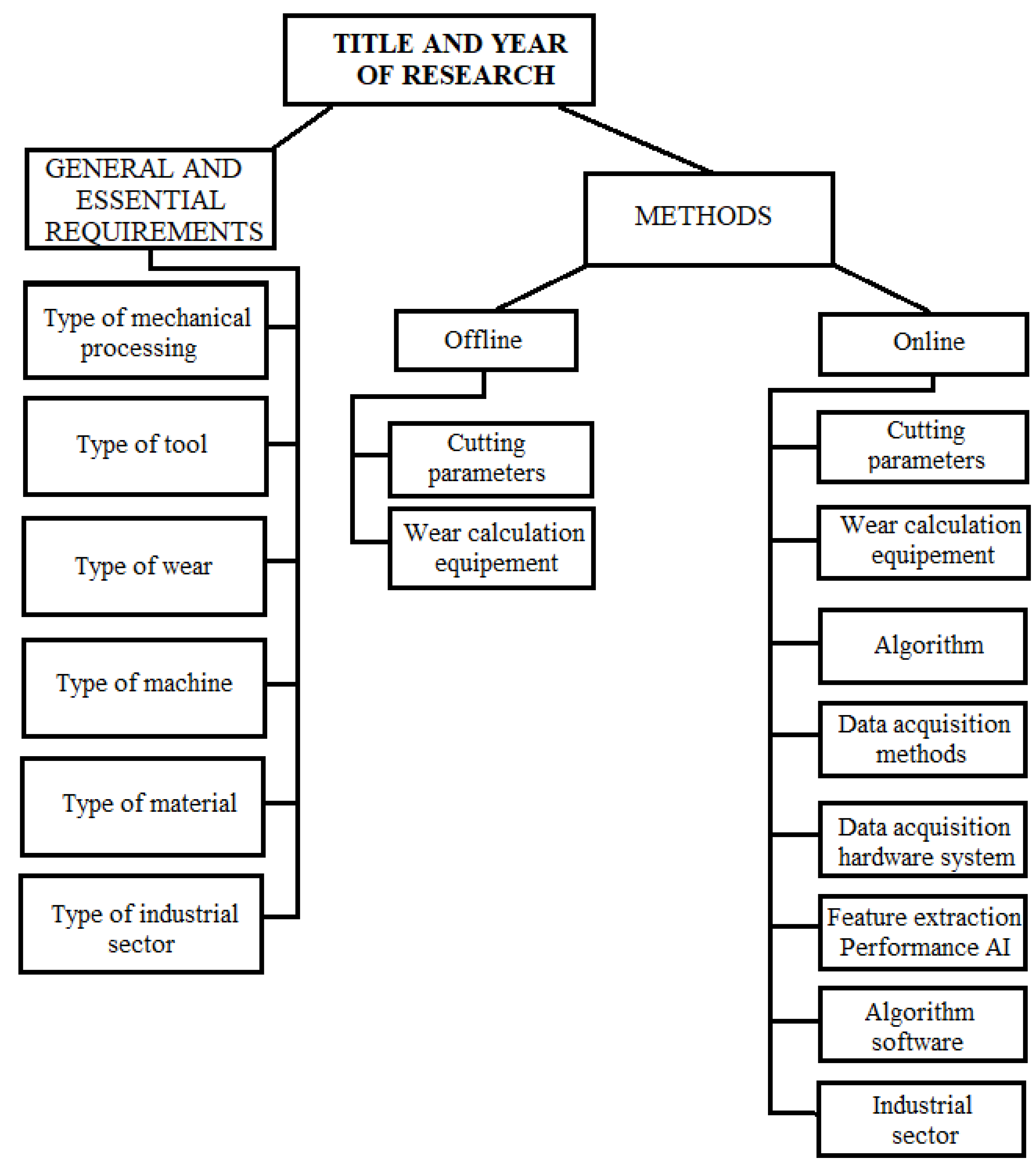
Figure 2.
Offline and online measurements [58].
Figure 2.
Offline and online measurements [58].
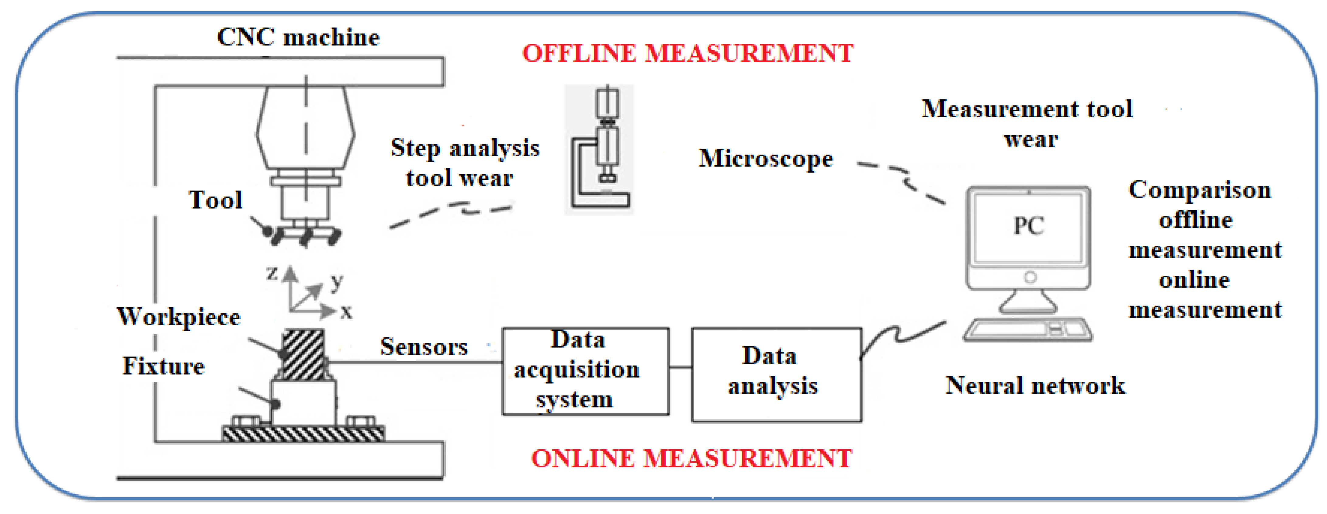
Figure 3.
Online measurement scheme.

Figure 4.
Number of publications on milling containing features of signal in different domains.
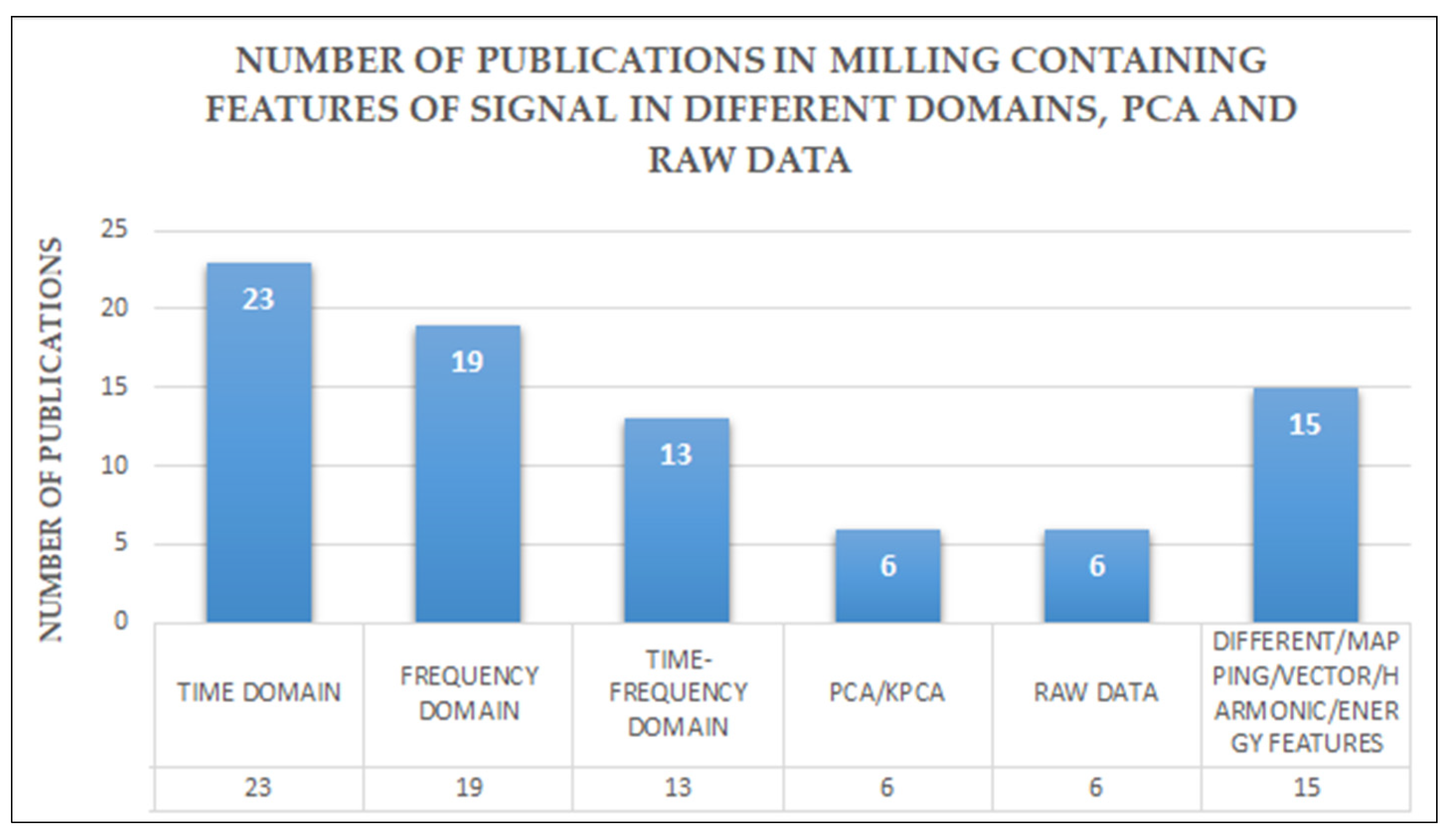
Figure 5.
Number of publications on turning containing features of signal in different domains.

Figure 6.
Number of publications on drilling containing features of signal in different domains.

Figure 7.
Number of publications containing AI per year.

Figure 8.
Number of publications containing type of AI.

Figure 9.
Number of publications on milling containing the type of AI.

Figure 10.
Number of publications on milling containing the type of signal.

Figure 11.
Number of publications on milling containing the type of wear.

Figure 12.
Number of publications for SVM in milling containing the type of wear.

Figure 13.
Number of publications for SVM in milling containing the type of wear.
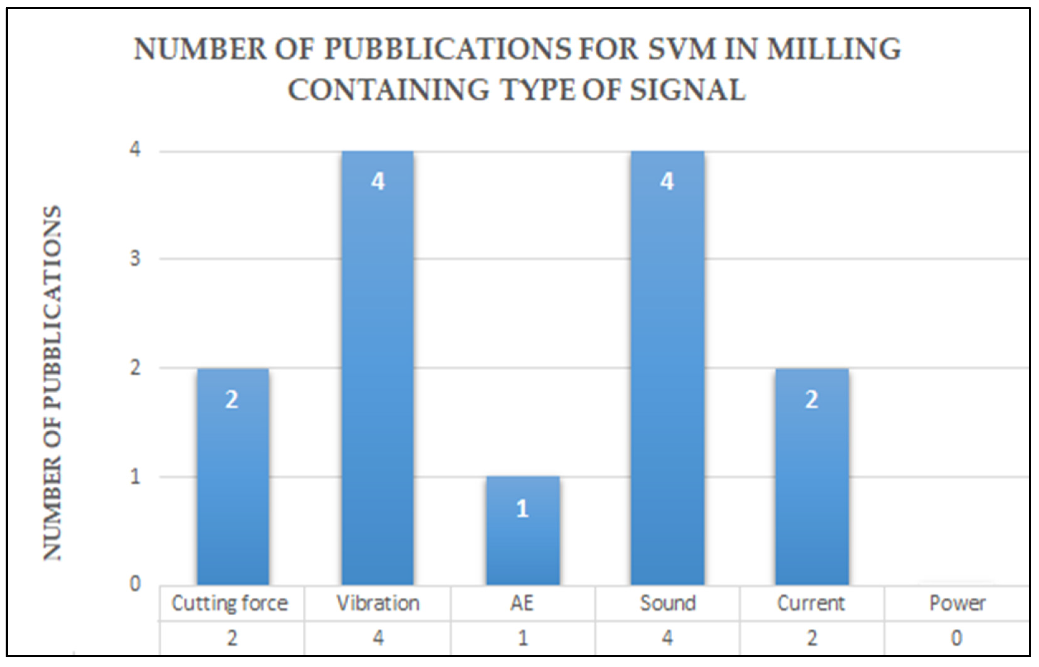
Figure 14.
Number of publications for SVM in milling containing the type of domain.
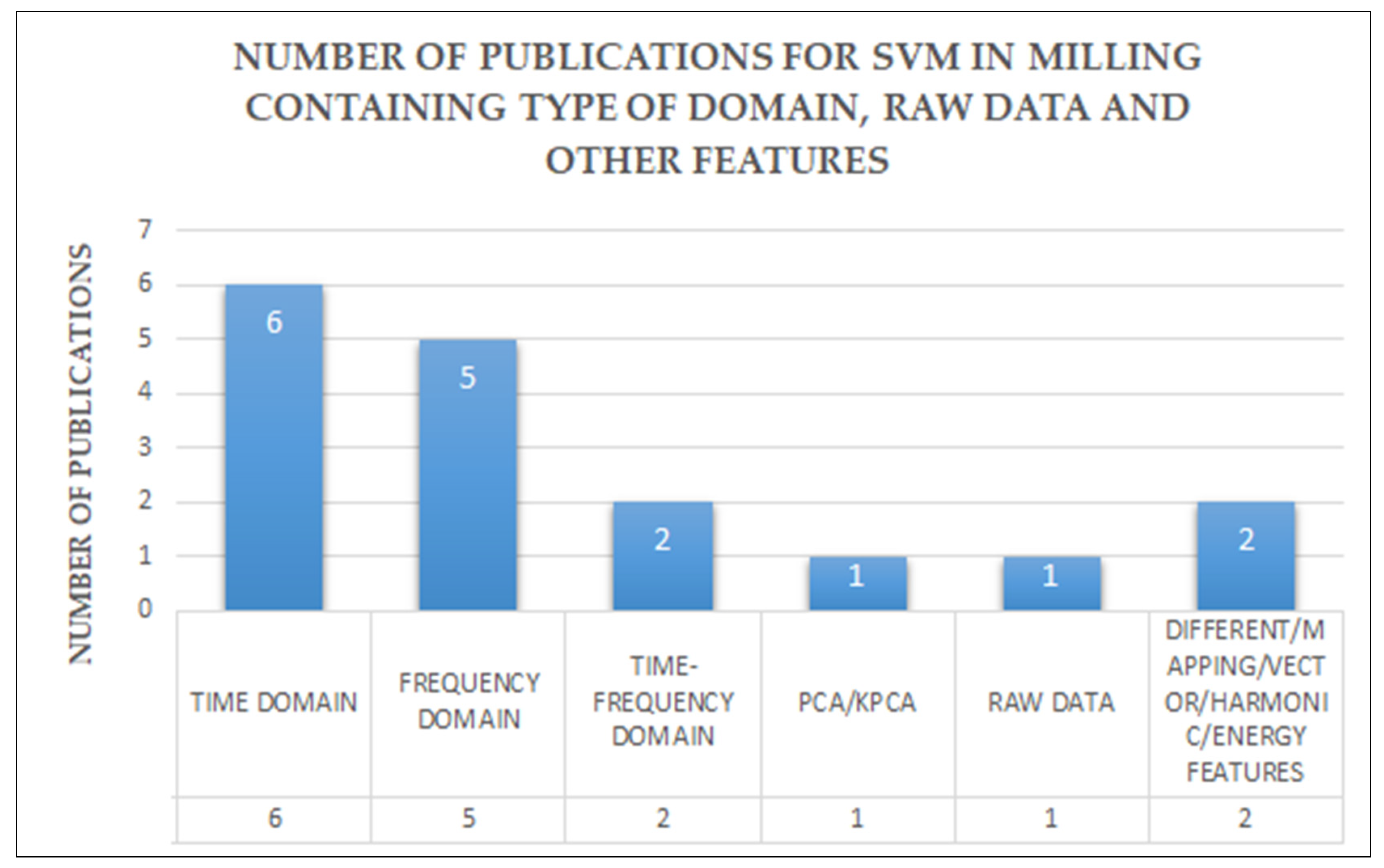
Figure 15.
Number of publications on turning containing the type of AI.

Figure 16.
Number of publications on turning containing the type of signal.
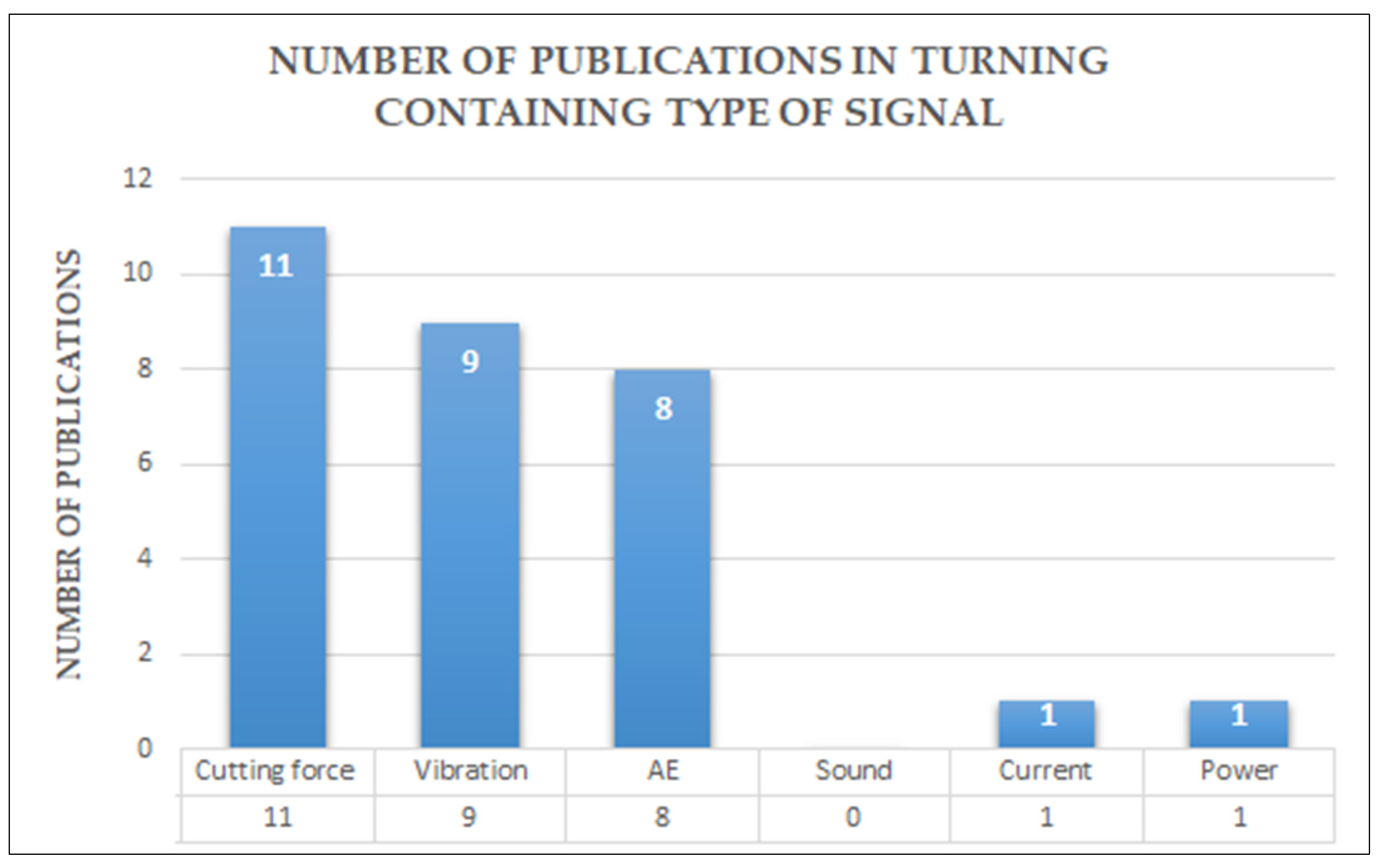
Figure 17.
Number of publications on turning containing the type of wear.

Figure 18.
Number of publications for ANN on turning containing the type of wear.

Figure 19.
Number of publications for ANN on turning containing the type of signal.
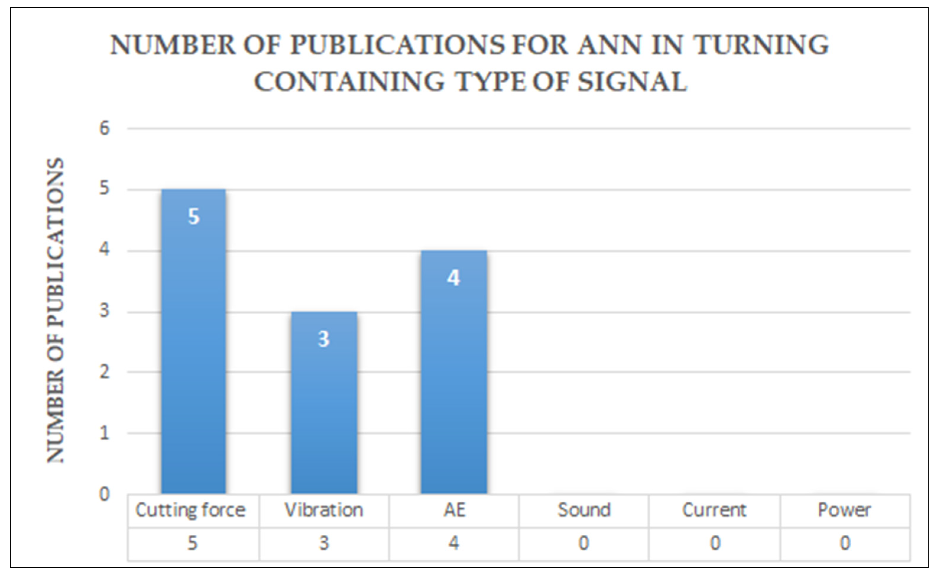
Figure 20.
Number of publications for ANN on turning containing the type of domain.

Figure 21.
Number of publications on drilling containing the type of AI.
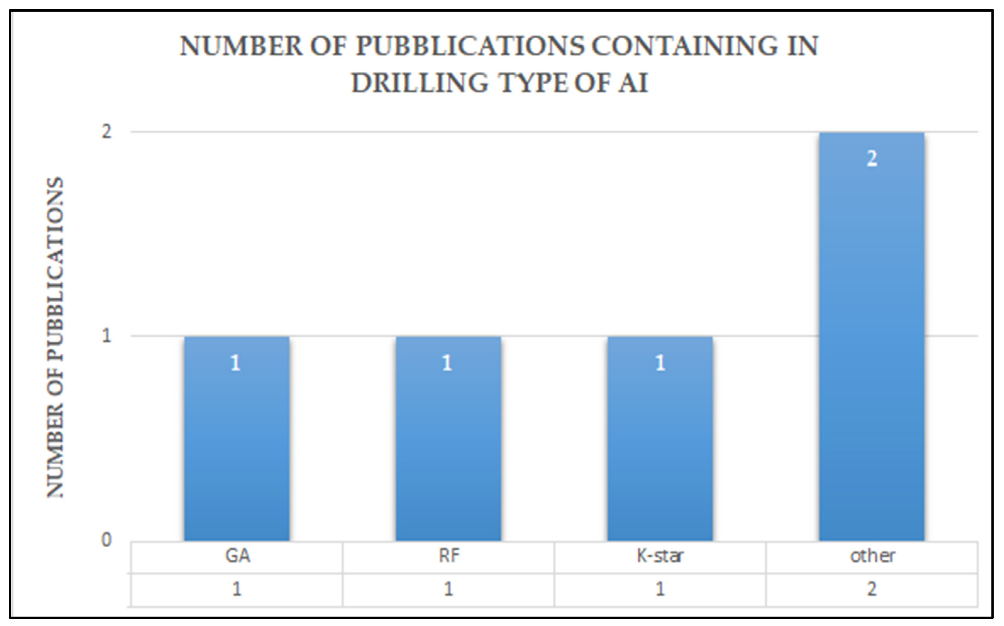
Figure 22.
Number of publications on drilling containing the type of signals.
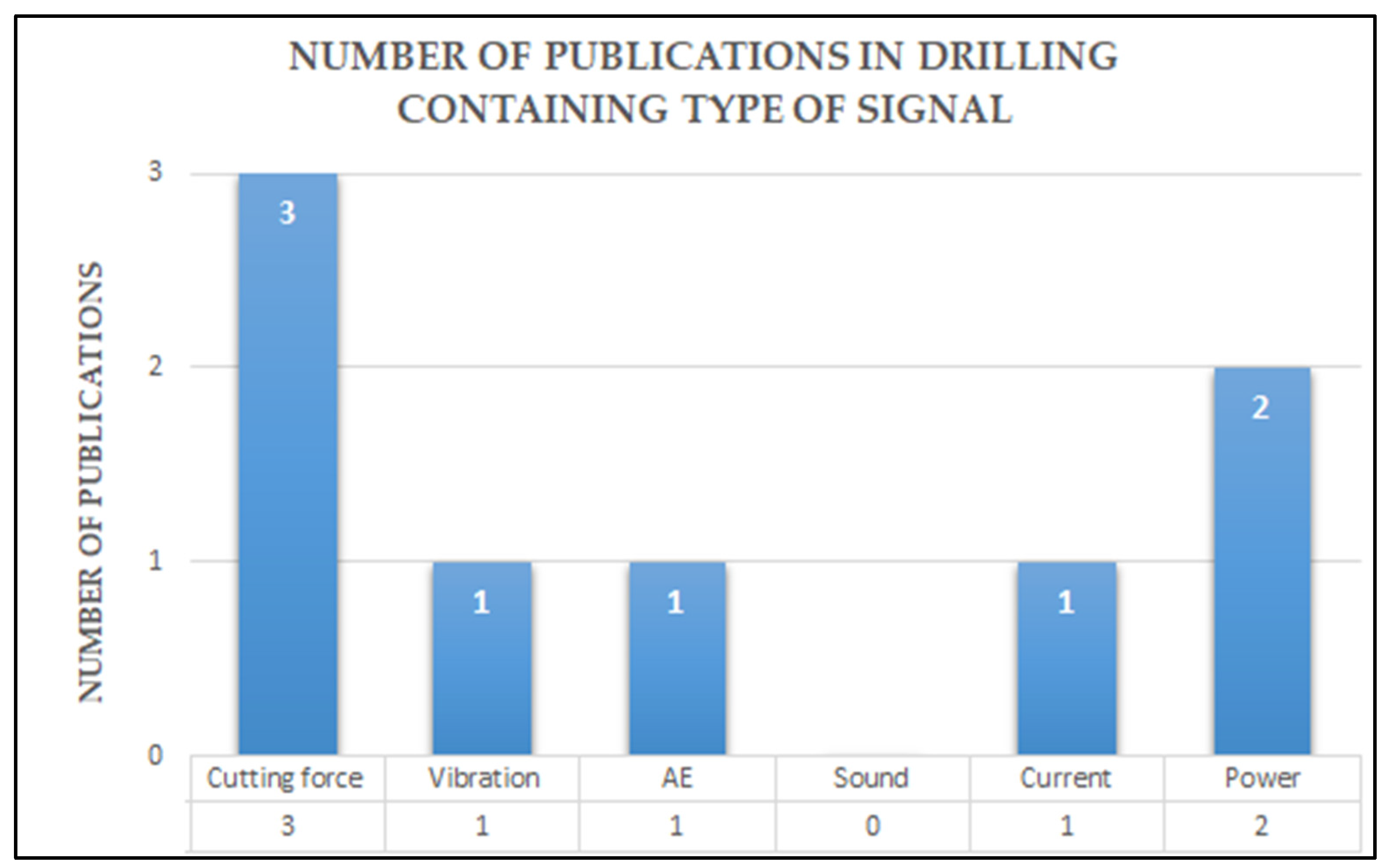
Figure 23.
Number of publications on drilling containing the type of wear.

Table 1.
Research level, research items and number of published articles found.
| Research Level | Items | Total Articles Found | Database Reasearch |
|---|---|---|---|
| FIRST | Research title: tool wear Years of publication: 2010–2020 Thematic areas: engineering Type of article: review article and research article | 21,760 | SCOPUS, GOOGLE SCHOLAR, WEB OF SCIENCES. Based on DOI |
| SECOND | Research title: tool wear monitoring, learning Years of publication: 2010–2020 Thematic areas: engineering Type of article: review article and research article | 2959 | |
| THIRD | Research title: tool wear monitoring, learning Years of publication: 2010–2020 Thematic areas: engineering, no micro cutting Type of article: review article and research article | 116 | |
| FOURTH | Research title: tool wear monitoring, learning Years of publication: 2010–2020 Thematic areas: engineering, no micro cutting, only metal materials Type of article: review article and research article | 97 | |
| FIFTH | Research title: tool wear monitoring, learning Years of publication: 2010–2020 Thematic areas: engineering, no micro cutting, only metal materials Type of article: review article and research article. In direct and indirect methods of tool wear measurement, measurement through images, i.e., cameras, optical measurements, is not considered | 77 |
Table 2.
General and essential requirements.
| General and Essential Requirements | |||||
|---|---|---|---|---|---|
| Machining Operations | Articles | Type of Wear | Type of Tool | Type of Material | Type of Machine |
| Milling | [8] | VB | high speed steel mill | Super alloy: Titanium alloy | vertical machine |
| Drilling | [9] | VB | carbide drill | Super alloy and Steel: Inconel718 and C45 | vertical machine |
| Milling | [10] | VB | high speed steel mill | Alluminium: Hardened 6061 | vertical machine |
| Milling | [11] | VB | insert mill | Alluminium: alluminimu alloy | vertical machine |
| Milling | [12] | VB and RUL | insert mill | / | vertical machine |
| Milling | [13] | VB | carbide mill | Alluminium: 6061 alluminium | vertical machine |
| Milling | [14] | VB | insert mill | Super alloy: Titanium alloy | vertical machine |
| Milling | [15] | VB | insert mill | / | vertical machine |
| Milling | [16] | VB | insert mill | Super alloy: Inconel 718 | vertical machine |
| Milling | [17] | VB | insert mill | Steel: C45 | vertical machine |
| Turning | [18] | VB | cemented carbide tool inserts | / | lathe machine |
| Milling | [19] | VB | insert mill | Super alloy: Ti6Al4V | vertical machine |
| Milling | [20] | VB | carbide mill | Steel: Stainless steel | vertical machine |
| Turning | [21] | VB | uncoated carbide inserts CNMG120408 | Super alloy: Inconel 718 | lathe machine |
| Milling | [22] | VB | high speed steel mill | Alluminium: aluminum alloys 5053-H111, 6082-T6, 2024-T3, 7022-T6, 7075-T6 | vertical machine |
| Turning | [23] | VB | tool inserts TNMM 110408 P25 | Steel: 42CrMo4 | lathe machine |
| Turning | [24] | VB | insert CNMG120404-MB NC30P grade 5 | Steel: JIS S45C carbon steel | lathe machine |
| Milling | [25] | VB | insert mill | / | vertical machine |
| Turning | [26] | VB | coated carbide insert CNMG120408 SM 1105 | Super alloy: Inconel 718 | lathe machine |
| Milling | [27] | VB | insert mill | Super alloy: Ti-6AI-4V | vartical machine |
| Turning | [28] | VB | turning tool | Super alloy: Inconel 718 | lathe machine |
| Drilling | [29] | VB | high speed steel drill | Super alloy: Inconel 625 | vertical machine |
| Turning | [30] | VB | carbide insert TNMG160408 | Steel: Mild steel | lathe machine |
| Turning | [31] | VB | carbide insert CNMG120408 MF1 CP200 | Super alloy: Titanium Metal matrix Composite (Ti MMC) 10 wt% TiC/Ti-6Al-4V | lathe machine |
| Milling | [32] | VB | insert mill | Super alloy: Titanium alloy Ti-5Al-5Mo-5V-1Cr-1Fe | vertical machine |
| Milling | [33] | VB | carbide mill | Steel: steel block of S235JR | vertical machine |
| Milling | [34] | VB | insert mill | Super alloy: Ti-6Al-4V | vertical machine |
| Milling | [35] | VB | insert mill | Super alloy: Ti-6Al-4V | vertical machine |
| Turning | [36] | VB | coated sintered carbide insert SNUN120408 | / | lathe machine |
| Milling | [37] | VB | high speed steel mill | Alluminium:6082 Alluminium | vertical machine |
| Milling | [38] | VB and RUL | carbide mill | Super alloy: Titanium alloy | vertical machine |
| Milling | [39] | RUL | carbide mill | Super alloy: Titanium alloy | vertical machine |
| Turning | [40] | VB | Uncoated carbide inserts SPGN 422, grade K68. Ceramic inserts Greenleaf SNGN 452, grade WG-300 | Steel and Super alloy: 4140 steel (HRC35), Inconel 718 and Ti-6Al-4V | lathe machine |
| Milling | [41] | VB and RUL | insert mill | Steel: stainless-steel | vertical machine |
| Milling | [42] | VB | carbide mill | Stell and Super alloy: C45 steel, Inconel 718 | vertical machine |
| Drilling | [43] | VB | carbide drill | / | vertical machine |
| Milling | [44] | VB | insert mill | Steel: 1018 steel at 121 HB hardness | vertical machine |
| Milling | [45] | VB, breakage and chipping | insert mill | Steel: 42CrMo4 | vertical machine |
| Milling | [46] | VB | insert mill | Steel: 1018 steel at 121 HB hardness | vertical machine |
| Milling | [47] | VB | carbide mill | / | vertical machine |
| Milling | [48] | VB and tool breakage. | high speed steel mill | Steel: 1040 cold rolled steel | vertical machine |
| Drilling | [49] | VB | high speed steel drill | Steel: AISI 316 stainless steel plate | vertical machine |
| Milling | [50] | VB | insert mill | Steel: stainless steel, HRC52 | vertical machine |
| Drilling | [51] | VB | high speed steel drill | Steel: mild-steel | vertical machine |
| Milling | [52] | VB and roughness | insert mill | Stell and Super alloy: H13 steel and Inconel 718 | vertical machine |
| Milling | [53] | VB | insert mill | Super alloy: titanium alloy | vertical machine |
| Milling | [54] | VB | insert mill | / | vertical machine |
| Milling Turning Drilling | [55] | VB, RUL chipping, breakage, corner wear, rake wear, notch wear | milling tool, turning tool, drilling tool | Ti- and Ni-based alloys, hardened steels, aluminum alloys | vertical machine, turning machine |
| Milling | [56] | VB and RUL | insert mill | cast iron: cast iron and stainless steel J45 | vertical machine |
| Milling | [57] | RUL | insert mill | cast iron: cast iron and stainless steel J45 | vertical machine |
| Milling | [58] | VB | carbide mill | Steel: stainless steel, HRC52 | vertical machine |
| Turning | [59] | VB | carbide insert | Steel: AISI 316 stainless steel | lathe machine |
| Milling | [60] | VB | carbide mill | Steel: material AISI M3:2, hardened to 62 HRC | vertical machine |
| Milling | [61] | VB | carbide mill | Super alloy: Ti-6Al-4V titanium | vertical machine |
| Milling | [62] | VB | carbide mill | Steel: Tempered steel C45 | vertical machine |
| Milling | [63] | VB | insert mill | Super alloy: Ti6Al4V alloy | vertical machine |
| Milling | [64] | VB | insert mill | Super alloy: Ti–6Al–4V | vertical machine |
| Milling | [65] | VB | carbide mill | Super alloy: Inconel 718 | vertical machine |
| Turning | [66] | VB, roughness and breakage | turning tool | Metal alloy | lathe machine |
| Milling | [67] | VB, breakage, light wear, middle wear, severe wear, sharp tool, worn tool, chipping | Carbide mill, insert mill, high speed steel mill | Super alloy, steel alloy and alluminium alloy | vertical machine |
| Turning | [68] | VB | Carbide insert CNMG-432 | Alluminium: aluminum alloy 6061 | lathe machine |
| Turning | [69] | VB | Carbide WNMG 084 08- QM | Steel alloy: stainless steel AISI 316 | lathe machine |
| Turning | [70] | Tool wear rate | uncoated carbide insert CCMT 060204 TT. | cast iron: cast iron (grey cast iron-FG 15) and an alloy steel (En 24) | lathe machine |
| Milling | [71] | VB | carbide mill | Super alloy: Inconel 718 | vertical machine |
| Milling | [72] | VB | insert mill | Steel: 1018 steel | vertical machine |
| Milling | [73] | VB | insert mill | Steel: 42CrMo4 | vertical machine |
| Milling | [74] | VB | insert mill | Steel: ASSAB718HH | vertical machine |
| Milling | [75] | VB | insert mill | cast iron: CGI 450 | vertical machine |
| Milling | [76] | RUL | carbide mill | Steel: tempered steel (HRC52) | vertical machine |
| Milling | [77] | tool wear status | insert mill | Super alloy: Ti-6Al-4V | vertical machine |
| Milling | [78] | tool wear rate, RUL | carbide mill | / | vertical machine |
| Turning | [79] | VB | ceramic insert CNMG120408-HM | Steel: C45 steel | lathe machine |
| Turning | [80] | VB | round ceramic inserts RNGN CC670 | Super alloy: Inconel 625 | lathe machine |
| Milling | [81] | VB | carbide mill | Super alloy; Inconel 718 | vertical machine |
| Turning | [82] | roughness | coated carbide insert TiCN/Al2O3/TiN | Steel: AISI 1060 | lathe machine |
| Turning | [83] | VB | carbide insert | Alluminium: alluminum alloy | lathe machine |
Table 3.
Cutting parameters of machining operations.
| Cutting Parameters | |||||||
|---|---|---|---|---|---|---|---|
| Machining Operations | Articles | Cutting SPEED | Spindle Speed | Depht of Cut, Radial Depht of Cut and Axial Depht of Cut | Feed, Feed Rate, Feed for Tooth | Diameter of Tool | Lubrificant |
| Milling | [8] | x | x | x | |||
| Drilling | [9] | x | |||||
| Milling | [10] | x | x | ||||
| Milling | [11] | x | x | x | |||
| Milling | [12] | x | x | x | |||
| Milling | [13] | x | x | ||||
| Milling | [14] | x | x | x | |||
| Milling | [15] | x | x | x | |||
| Milling | [16] | x | x | x | |||
| Milling | [17] | x | x | x | |||
| Turning | [18] | x | x | x | |||
| Milling | [19] | x | x | x | |||
| Milling | [20] | x | x | x | |||
| Turning | [21] | x | x | x | |||
| Milling | [22] | x | x | x | |||
| Turning | [23] | x | x | ||||
| Turning | [24] | x | x | x | |||
| Milling | [25] | x | x | ||||
| Turning | [26] | x | x | x | |||
| Milling | [27] | x | x | x | |||
| Turning | [28] | x | x | x | |||
| Drilling | [29] | x | x | ||||
| Turning | [30] | x | x | x | |||
| Turning | [31] | x | x | x | |||
| Milling | [32] | x | x | x | |||
| Milling | [33] | x | x | x | |||
| Milling | [34] | x | x | x | |||
| Milling | [35] | x | x | ||||
| Turning | [36] | x | |||||
| Milling | [37] | x | x | x | |||
| Milling | [38] | x | x | ||||
| Milling | [39] | x | x | x | |||
| Turning | [40] | x | x | x | |||
| Milling | [41] | x | x | x | |||
| Milling | [42] | x | x | x | |||
| Milling | [44] | x | x | ||||
| Milling | [45] | x | x | x | |||
| Milling | [46] | x | x | ||||
| Milling | [47] | x | x | x | |||
| Milling | [48] | x | x | ||||
| Drilling | [49] | x | x | x | |||
| Milling | [50] | x | x | x | |||
| Drilling | [51] | x | x | x | |||
| Milling | [52] | x | x | x | |||
| Milling | [53] | x | x | x | |||
| Milling | [54] | x | x | x | |||
| Milling Turning Drilling | [55] | x | x | x | x | ||
| Milling | [56] | x | x | x | |||
| Milling | [57] | x | x | ||||
| Milling | [58] | x | x | x | |||
| Turning | [59] | x | |||||
| Milling | [60] | x | x | ||||
| Milling | [61] | x | x | x | |||
| Milling | [62] | x | x | x | |||
| Milling | [63] | x | x | ||||
| Milling | [64] | x | x | x | |||
| Milling | [65] | x | x | x | |||
| Turning | [66] | x | x | x | |||
| Milling | [67] | x | x | x | |||
| Turning | [68] | x | x | x | |||
| Turning | [69] | x | x | ||||
| Turning | [70] | x | x | x | |||
| Milling | [71] | x | x | ||||
| Milling | [72] | x | x | x | |||
| Milling | [73] | x | x | x | |||
| Milling | [74] | x | x | x | |||
| Milling | [75] | x | x | x | |||
| Milling | [76] | x | x | x | |||
| Milling | [77] | x | x | x | |||
| Milling | [78] | x | x | x | |||
| Turning | [79] | x | x | x | |||
| Turning | [80] | x | x | x | |||
| Milling | [81] | x | x | x | |||
| Turning | [82] | x | x | x | |||
| Turning | [83] | x | x | x | |||
Table 4.
Sensor signals in turning articles.
| TURNING | Articles | Cutting Force Signal | Vibration | Acoustic Emission Signal | Sound | Current | Power | Number of Signals |
| [18] | x | 1 | ||||||
| [21] | x | x | x | 3 | ||||
| [23] | x | 1 | ||||||
| [24] | x | x | 2 | |||||
| [26] | x | x | 2 | |||||
| [27] | x | 1 | ||||||
| [28] | x | x | x | 3 | ||||
| [30] | x | 1 | ||||||
| [31] | x | 1 | ||||||
| [36] | x | 1 | ||||||
| [40] | x | x | 2 | |||||
| [59] | x | x | x | 3 | ||||
| [68] | x | x | 2 | |||||
| [70] | x | x | 2 | |||||
| [79] | x | x | x | 3 | ||||
| [80] | x | x | x | 3 | ||||
| [83] | x | x | 2 |
Table 5.
Sensor signals in milling articles.
| Articles | Cutting Force Signal | Vibration | Acoustic Emission Signal | Sound | Current | Power | Number of Signals |
|---|---|---|---|---|---|---|---|
| [8] | x | x | x | 2 | |||
| [10] | x | 1 | |||||
| [11] | x | 2 | |||||
| [12] | x | x | x | 3 | |||
| [13] | x | 1 | |||||
| [14] | x | 1 | |||||
| [15] | x | 1 | |||||
| [17] | x | x | 2 | ||||
| [19] | x | x | 2 | ||||
| [20] | x | 1 | |||||
| [22] | x | x | x | 3 | |||
| [25] | x | x | 2 | ||||
| [27] | x | 1 | |||||
| [32] | x | 1 | |||||
| [33] | x | 1 | |||||
| [34] | x | 1 | |||||
| [35] | x | 1 | |||||
| [37] | x | 1 | |||||
| [38] | x | x | 2 | ||||
| [39] | x | x | 2 | ||||
| [41] | x | x | x | 3 | |||
| [42] | x | x | x | 3 | |||
| [44] | x | 1 | |||||
| [45] | x | 1 | |||||
| [46] | x | 1 | |||||
| [47] | x | x | 2 | ||||
| [48] | x | 1 | |||||
| [50] | x | x | 2 | ||||
| [52] | x | 1 | |||||
| [53] | x | 1 | |||||
| [54] | x | 1 | |||||
| [56] | x | x | 2 | ||||
| [57] | x | x | x | 3 | |||
| [58] | x | x | 2 | ||||
| [60] | x | 1 | |||||
| [61] | x | 1 | |||||
| [62] | x | 1 | |||||
| [63] | x | 1 | |||||
| [64] | x | 1 | |||||
| [65] | x | 1 | |||||
| [71] | x | x | 2 | ||||
| [72] | x | 1 | |||||
| [73] | x | 1 | |||||
| [74] | x | x | 2 | ||||
| [75] | x | x | 2 | ||||
| [76] | x | 1 | |||||
| [77] | x | 1 | |||||
| [78] | x | x | x | 3 | |||
| [81] | x | x | x | 3 |
Table 6.
Sensor signals in drilling articles.
| Studies | Cutting Force Signal | Vibration | Acoustic Emission Signal | Sound | Current | Power | Number of Signals | |
|---|---|---|---|---|---|---|---|---|
| DRILLING | [9] | x | x | 2 | ||||
| [29] | x | x | 2 | |||||
| [43] | x | x | 2 | |||||
| [49] | x | 1 | ||||||
| [51] | x | 1 |
Table 7.
Milling, turning and drilling performances.
| Articles | Signal | A.I. Methods | Performance | Performance Data |
|---|---|---|---|---|
| [10] | Sound | CNN with SGD | Predictive accuracy | (1) CNN predictive accuracy 81% |
| [11] | Current | SVM, LDA; KNN, NN, NB, DT | Accuracy | (1) SVM accuaracy 90% (2) LDA accuaracy 90% (3) DT accuaracy 84.1% (4) BN accuaracy 85% (5) NN accuaracy 85% |
| [12] | Cutting force, vibration and acoustic emission | HMM | MAPE, Mean and Accuracy | (1) HMM MAPE = 25.05 for 68% confidence level; (2) HMM MAPE = 18.37 for 95% confidence level; (3) HMM MAPE = 39.68 for 99.7% confidence level |
| [13] | Sound | CART, RF, KNN, SVM with EBCA and without EBCA | Accuracy without EBCA Accuracy with EBCA Accuracy with training set 50–60–70–80% | (1) Accuracy obtained CART, RF, KNN, SVM without EBCA about 94% (2) Accuracy obtained CART, RF, KNN, SVM with EBCA about 96% (3) CART, RF, KNN, SVM: - training set 50% accuracy from 93 to 95% - training set 60% accuracy from 96 to 97% - training set 70% accuracy from 97 to 98% - training set 80% accuracy from 98 to 99% |
| [16] | Cutting force | ANN | R, MRE, R² | (1) ANN R 0.992, (2) ANN MRE 5.42%, (3) ANN R² 0.996 |
| [19] | Cutting force,vibration | EAM ARTMAP, FUZZY ARTMAP (FAM) | Averaging recognition rate | (1) EAM averaging recognition rate 98.67% (2) FAM averaging recognition rate 89.67% |
| [20] | Cutting force | CNN, AC | Predicted Rapid initial wear, Predicted Uniform wear, Predicted Failure wear Accuracy % | (1) CNN accuarcy 90% |
| [27] | Cutting force | RVM with KPCA-IRBF | RMSE, CI_widht/CI_var | (1) KPCA_IRBF can reduce the mean square error (RMSE) of RVM by more than 30%. (2) mean width of CI by more than 90% |
| [34] | Cutting force | Kalman filter | RMSE | (1) RMSE decreases when force data is taken from the measured signal equation. |
| [35] | Acoustic emission | CRF and HMM | Accuracy rate | (1) The accuracy rate of the HMM is lower than the CRF model for each state of tool wear |
| [39] | Cutting force, current | SVM, RF and feedforrward NN | Score, RMSE and Accuracy | (1) RF score 64.04 (2) RF accuaracy 71% (3) RMSE indicating prediction error decreases by 4% and 12% with respect to SVR and feedforward NN |
| Articles | Signal | A.I. Methods | Performance | Performance Data |
| [44] | Sound | GAN | Accuracy, non-conforming tool | (1) GAN accuracy 90.56% (2) GAN non-confroming tool reduced from 16.65% to 4.52% |
| [45] | Vibration | K-star | Positive rate (TP rate) and False positive rate (FP rate) and Accuracy | K-star accuracy 96.5 % |
| [46] | Sound | DCNN | Accuracy | DCNN accuracy from 81% to 100% |
| [52] | Power | NN inconrporate CNN and RNN NN incorporate RNN | Accuracy | (1) NN (CNN and RNN) accuracy from 82% to 90% (2) NN (RNN) accuracy 85% |
| [53] | Cutting force | ARTMAP (GAM) | accuracy | ARTMAP (GAM) accuracy from 89% to 100% |
| [61] | Cutting force | DE-SVR | Accuracy VB and Acccuracy RUL | (1) DE-SVR accuracy VB 88% (2) DE-SVR accuracy RUL 88.5% |
| [62] | Sound | SVM | Maximum shape error | SVM maximum shape error 70% |
| [63] | Vibration | SVM with TIPM SVM without TIPM | Accuracy | (1) SVM with TIPM accuracy 90.8 % (2) SVM with TIPM accuracy 81.9 % |
| [64] | Vibration | SVM | RMSE and Accuracy | (1) SVM RMSE 0.00475 (2) SVM Accuracy 99.6% |
| [18] | Cutting force | KPCA_IRBF | CI | (1) KPACA_IRBF CI 95% |
| [21] | Cutting force, torque, vibration acoustic emission | NN | SR | (1) NN SR force + AE 92.2 % (2) NN SR torque + AE 87.8% (3) NN SR torque + force + AE 98.9% |
| [24] | Cutting force, vibration | ANFIS algorithm | Minimum MAPE Maximum MAPE Average MAPE | In the ANFIS, MAPE depends on cutting speed vc, cutting diameter Dc and feed speed f. (1) Vc 200 mm/min Dc 1.6 mm f 0.25 mm/rev Minimum MAPE 0,48% Maximum MAPE 5.59% Average MAPE 2.3 % (2) Vc 250 mm/min Dc 1.2 mm f 0.25 mm/rev Minimum MAPE 0,96% Maximum MAPE 14.29% Average MAPE 5.08 % (3) Vc 300 mm/min Dc 0.8 mm f 0.25 mm/rev Minimum MAPE 0% Maximum MAPE 19.64% Average MAPE 4.07 % |
| [28] | Cutting force, vibration and acoustic emission | NN with PCA | SR | (1) NN SR between 79% and 98%. (2) NN Only cutting force signals SR 92%. (3) NN Only the three accelerations SR 81% (4) NN Torque and the three cutting forces SR 93% (5) NN Torque with the three accelerations SR 83% |
| [30] | Vibration | K-star | TP rate’ and ‘FP rate define the accuracy | (1) K-star accuracy 78% |
| [68] | Vibration and emission acoustic | ANN | Accuracy | ANN accuracy from 73.65% to 87.78% |
| [43] | Current and power | RF | Accuracy, R², MAE,RMSE | RF accuracy from 84% to 97.4% (1) R² 0.74 (2) RMSE 5.11 (3) MAE 4.25 microns |
| [49] | Vibration | K-star | Accuracy | (1) K-star accuracy 79.56% |
| [51] | Cutting force | RBFN with GA | MSE and % MSE | (1) RBFN MSE 2.0236% |
Disclaimer/Publisher’s Note: The statements, opinions and data contained in all publications are solely those of the individual author(s) and contributor(s) and not of MDPI and/or the editor(s). MDPI and/or the editor(s) disclaim responsibility for any injury to people or property resulting from any ideas, methods, instructions or products referred to in the content. |
© 2023 by the authors. Licensee MDPI, Basel, Switzerland. This article is an open access article distributed under the terms and conditions of the Creative Commons Attribution (CC BY) license (https://creativecommons.org/licenses/by/4.0/).
Share and Cite
MDPI and ACS Style
Munaro, R.; Attanasio, A.; Del Prete, A. Tool Wear Monitoring with Artificial Intelligence Methods: A Review. J. Manuf. Mater. Process. 2023, 7, 129. https://doi.org/10.3390/jmmp7040129
AMA Style
Munaro R, Attanasio A, Del Prete A. Tool Wear Monitoring with Artificial Intelligence Methods: A Review. Journal of Manufacturing and Materials Processing. 2023; 7(4):129. https://doi.org/10.3390/jmmp7040129
Chicago/Turabian StyleMunaro, Roberto, Aldo Attanasio, and Antonio Del Prete. 2023. "Tool Wear Monitoring with Artificial Intelligence Methods: A Review" Journal of Manufacturing and Materials Processing 7, no. 4: 129. https://doi.org/10.3390/jmmp7040129