A Novel Heterogeneous Swarm Reinforcement Learning Method for Sequential Decision Making Problems


1
Institute for Computer Science and Business Information Systems (ICB), University of Duisburg-Essen, 45141 Essen, Germany
2
Department of Information Systems, Poznan University of Economics and Business, 61-875 Poznan, Poland
*
Author to whom correspondence should be addressed.
Mach. Learn. Knowl. Extr. 2019, 1(2), 590-610; https://doi.org/10.3390/make1020035
Submission received: 12 March 2019
/
Revised: 10 April 2019
/
Accepted: 12 April 2019
/
Published: 16 April 2019
(This article belongs to the Section Learning)
Abstract
:Sequential Decision Making Problems (SDMPs) that can be modeled as Markov Decision Processes can be solved using methods that combine Dynamic Programming (DP) and Reinforcement Learning (RL). Depending on the problem scenarios and the available Decision Makers (DMs), such RL algorithms may be designed for single-agent systems or multi-agent systems that either consist of agents with individual goals and decision making capabilities, which are influenced by other agent’s decisions, or behave as a swarm of agents that collaboratively learn a single objective. Many studies have been conducted in this area; however, when concentrating on available swarm RL algorithms, one obtains a clear view of the areas that still require attention. Most of the studies in this area focus on homogeneous swarms and so far, systems introduced as Heterogeneous Swarms (HetSs) merely include very few, i.e., two or three sub-swarms of homogeneous agents, which either, according to their capabilities, deal with a specific sub-problem of the general problem or exhibit different behaviors in order to reduce the risk of bias. This study introduces a novel approach that allows agents, which are originally designed to solve different problems and hence have higher degrees of heterogeneity, to behave as a swarm when addressing identical sub-problems. In fact, the affinity between two agents, which measures the compatibility of agents to work together towards solving a specific sub-problem, is used in designing a Heterogeneous Swarm RL (HetSRL) algorithm that allows HetSs to solve the intended SDMPs.
1. Introduction
Decision making tasks that involve delayed consequences can be formulated as sequential decision making problems, for which decision making strategies must be found that take into account the expectations of both short-term and long-term consequences of the decisions. Dealing with such problems, at each time step, the Decision Maker (DM), observes the system’s current state and selects an action, and then makes a transition to a successor state, which is determined by the current state, the chosen action, and a random disturbance that aims at the exploration–exploitation trade-off. For each action, the DM will then receive a certain amount of payoff that depends on the action and the current state. The goal is to find a rule, i.e., an action selection policy, for the DM that maximizes the total amount of the accumulated payoff.
Markov Decision Processes (MDPs) [1] provide a framework for modeling such sequential decision making problems. The optimization problem is solved by applying the Dynamic Programming (DP) approach and Reinforcement Learning (RL). Some algorithms for sequential decision making have been studied in Reference [2], which aim to produce policies that maximize the long-term reward an agent receives in its environment. According to the authors of Reference [2], based on the information available for producing these policies they can be constructed under two different problem scenarios: Planning and Reinforcement Learning. Planning is used when a complete model of the environment is known in advance and the produced policy is typically stationary. In reinforcement learning, however, a model of the environment is unknown or difficult to work with directly. This study concentrates on such problem scenarios.
The application of RL to an MDP allows a single agent to learn a policy that maximizes a cumulative reward that is received from the environment. However, when multiple agents apply RL in a shared environment, the optimal policy of an agent depends not only on the environment, but on the actions of the other agents as well. In this case, there are two main groups to be considered: Multi-agent systems, consisting of agents that have an individual goal and decision making capabilities, which are influenced by other agent’s decisions, and on the other hand multi-agent systems that behave as a swarm, consisting of agents that collaboratively learn a single objective. The Multi-Agent RL (MARL) is based on Game Theory concepts, which induces agents to be capable of discovering good solutions to the problem at hand either by coordinating with other learners or by competing with them. However, swarm RL considers Swarm Intelligence (SI) concepts, allowing the agent to share their knowledge by updating the policy the swarm is following. This study focuses on the latter category.
The term Swarm Intelligence (SI), first introduced in Reference [3], refers to the self-organized collective behavior of natural and artificial systems composed of many individuals following simple rules that exploit only local information. Examples of natural systems exhibiting swarm intelligence are colonies of ants and termites, schools of fish, flocks of birds, and herds of land animals. Inspired by the natural systems, some artificial systems are also benefiting from the power of swarm intelligence, notably some multi-robot systems (e.g., Reference [4]), and also certain computer programs that are developed to solve optimization and data analysis problems (e.g., Reference [5]). The artificial SI systems consist typically of a population of simple robots or software agents. However, recently, some SI systems have been developed that allow human swarming (e.g., Reference [6]).
A typical swarm intelligence system has the following properties [7]:
- it consists of many individuals;
- the individuals are relatively homogeneous, i.e., they are either identical of they belong to a small number of typologies;
- the individuals exhibit stigmergy, i.e., they interact based on simple behavioral rules that exploit solely local information that the individuals exchange directly or via their environment;
- the overall behavior of the system self-organizes, i.e., it results from the interactions of the individuals with each other or with the environment.
Homogeneous swarms are attractive due to their conceptual simplicity [8], thus most existing studies consider homogeneous swarms. However, real-world swarms often include agents with varying dynamical properties, which leads to new collective behaviors [9]. This heterogeneity ranges from intra-species behavioral variations caused by morphologic or age differences, to inter-species cooperation, such as symbiosis [8]. In Reference [8] interesting examples of heterogeneous natural systems are given:
- Age-structured swarms, in which heterogeneity arises when motion or sensing capabilities vary significantly with age.
- Predator–prey swarming, where there are distinct time-scale differences in the motion of predator and prey animals.
- Segregation of intermingled cell types during growth and development of an organism by introducing heterogeneity in inter cell adhesion properties.
Inspired by heterogeneous natural swarms, heterogeneous artificial swarms have also been designed and implemented. Some notable studies in this field have concentrated on robotic systems, where individual robots with varying capabilities are segregated in two to three populations and then are used together in order to achieve a common goal [4,9,10,11,12]. The varying capabilities that causes the heterogeneity in such systems may be due to the lack of capabilities that are costly to be implemented in all agents, or may arise over time, when some agents in the swarm malfunction [9]. Heterogeneity has also been used in approaches based on Particle Swarm Optimization (PSO) technique [8,13,14]. According to Reference [8], in this technique, differences along any of the aspects of the configuration of a particle give rise to a taxonomy based on four types of heterogeneity: Neighborhood heterogeneity, model-of-influence heterogeneity, update-rule heterogeneity, and parameter heterogeneity.
Heterogeneous systems have also attracted many researchers differently as designing task-specific agents is often easier than designing versatile, multipotent ones [8]. In order to keep a swarm homogeneous all the agents should be equipped with all the capabilities needed, which would in many cases eventually lead to complicated agents. Hence, heterogeneity clearly supports the very important property of the SI systems and that why in such systems the agents are to be kept as simple as possible.
As mentioned, so far, systems introduced as Heterogeneous Swarms (HetSs) merely include very few, i.e., two or three sub-swarms of homogeneous agents, which either according to their capabilities, deal with a specific sub-problem of the general problem (e.g., Reference [4]), or exhibit different behaviors in order to try a variety of different approaches to the same problem, and hence reduce the risk of using a homogeneous swarm of the wrong type for the problem at hand [8]. This study introduces a novel approach that allows agents, which are originally designed to solve different problems and hence have higher degrees of heterogeneity, to behave as a swarm when addressing identical sub-problems. In fact, if there is an overlap between the problems two different agents are solving, or between the data they are aiming for, they may have valuable knowledge to share and hence a reason to behave as a swarm. This work will focus on swarm Reinforcement Learning (RL) methods and introduces a technique to be used by heterogeneous group of agents with diverse but overlapping goals in order to exhibit swarm behavior.
The rest of the paper is organized as follows. Section 2 briefly describes the MDPs, and Section 3 goes over the RL methods for MDPs. Section 4 concentrates on Heterogeneous Swarm RL (HetSRL) and the original contribution of this research. In Section 5 and Section 6, examples of the usage of the proposed HetSRL method are given and Section 7 concludes with a summary and some directions for future research.
2. Markov Decision Processes (MDPs)
2.1. Formal MDP Definition
Markov Decision Processes (MDPs), also referred to as stochastic dynamic programs or stochastic control problems, are models for sequential decision making when outcomes are uncertain [1]. They are defined as controlled stochastic processes satisfying the Markov property and assigning reward value to state transitions [1]. A stochastic process has the Markov property if the conditional distribution of the next state of the process depends only on the current state of the process [15].
A Markov decision process consists of decision epochs, states, actions, rewards, and transition probability functions. In each state, after choosing an action a reward is received, which can, through a transition probability function, determine the state at the next decision epoch [1]. According to Reference [16], a Markov Decision Process (MDP) is a model of an agent operating in an uncertain but observable world. The definition of Markov Decision Process presented here and the notations are according to the ones used in Reference [16] and Reference [17].
Formally, an MDP is a 5-tuple :
- is a set of agent-environment states.
- is a set of actions the agent can take.
- is a state transition function which gives the probability that taking action in state results in state .
- is a reward function that quantifies the reward the agent gets for taking action in state resulting in state .
- is a discount factor that trades off between immediate reward and potential future reward.
In the MDP model, the world is one state at any given time. The agent fully observes the true state of the world and itself. At each time step, the agent chooses and executes an action from its set of actions. The agent receives some reward based on the reward function for its action choice in that state. The world then probabilistically transitions to a new state according to the state transition function. The objective of the MDP agent is to act in a way that allows it to maximize its future expected reward. The solution to an MDP is known as a policy, , a function that maps states to actions. The optimal policy over an infinite horizon is one inducing the value function:
This famous equation, known as the “Bellmann Equation”, quantifies the value of being in a state based on an immediate reward as well as a discounted expected future reward. The future reward is based on what the agent can do from its next state and the reward of future states it may move to, discounted more as time increases. The recursion specifies a dynamic program, which breaks the optimization into subproblems that are solved sequentially in a recurrent fashion.
In other words, the core problem of MDPs is to find a policy for the decision maker that is a rule that the agent follows in selecting actions, given the state it is in: A function that specifies the action which the decision maker will choose when in state . A policy is therefore a way of defining the agent’s action selection with respect to changes in the environment. The goal is to choose a policy that will maximize some cumulative function of the random rewards, typically the expected discounted sum over a potentially infinite horizon.
According to Reference [18], we can formalize reinforcement learning in terms of Markov decision processes, but in which the agent, initially, only knows the set of possible states and the set of possible actions. Thus, the state transition function, , and the reward function, , are initially unknown. An agent can act in a world and, after each step, observe the state of the world and observe what reward it obtained. Assume the agent acts to achieve the optimal discounted reward with a discount factor .
According to Reference [19], the cumulative value , achieved by following an arbitrary policy from an arbitrary initial state , can be defined as follows:
where the sequence of rewards denoted by is received by beginning at the state and repeatedly applying the policy to select actions. The rewards are discounted exponentially by factor of . Note that if , only the immediate reward is considered and if is closer to 1, futures rewards are given greater emphasis in comparison with the immediate reward. The quantity defined in Equation (2) is called the discounted cumulative reward achieved by applying policy from initial state . The agent aims to learn a policy that maximizes for all states . Such a policy is called an optimal policy and is noted by .
To simplify the notation, the value function of such an optimal policy is referred to as (cf. Equation (1)).
Reinforcement learning algorithms aim to learn an optimal policy for an MDP, using solely the reward signals received through the iterating interactions with the environment. These algorithms can be divided into two classes: Value iteration and policy iteration algorithms. Value iteration algorithms in fact learn the optimal value function and attempt to derive an optimal policy from this learnt value function. Alternatively, policy iteration algorithms directly build an optimal policy. Generally, they consist of two interleaved phases: Policy evaluation and policy improvement. During the policy evaluation phase the value of the current policy is estimated. Based on this estimate the policy is then locally improved during the policy improvement phase. This process continues until no further improvement is possible and an optimal policy is reached [20].
2.2. The Exploitation–Exploration Trade-Off
Since RL algorithms do not assume a given model for the MDP, one of the key issues in applying them is that learners need to explore the environment in order to discover the effects of their actions. This implies that the agent cannot simply play the actions that have the current highest estimated rewards, but also needs to try new actions in an attempt to discover better strategies. This problem is usually known as the exploitation–exploration trade-off in RL [20]. Two basic approaches exist to address this problem. On-policy methods aim to evaluate and improve the policy that is being applied to make the decisions. Such methods essentially estimate the value of a policy while using it for control. In off-policy methods, however, these two functions are separated and the behavior policy, i.e., the policy that is used to generate the behavior, may in fact be unrelated to the estimation policy, which is the policy that is being evaluated and improved. An advantage of this separation is that the estimation policy may be deterministic, e.g., greedy, while the behavior policy can continue to explore all possible actions [17]. In other words, the algorithm learns the values associated with taking the exploitation policy while following an exploration/exploitation policy.
2.3. Action–Selection Strategies
As mentioned above, a common challenge in RL is to find a trade-off between exploration (attempting to discover new features about the world by a selecting sub-optimal action) and exploitation (using what we already know about the world to get the best results we know of) [21]. The agents may follow different action–selection strategies in order to choose their actions, each of them dealing differently with this trade-off:
Greedy action-selection: The simplest action-selection strategy is the greedy strategy, in which the agent always selects the action with the highest state-action value. This strategy implements pure exploitation, while the rest of the action-selection strategies aim to achieve a balance between exploration and exploitation.
ε-Greedy action-selection: ε-Greedy is a variation on a normal greedy action-selection strategy. In both strategies, the agent believes that the best move is the one with the highest state-action value. However, in ε-greedy strategy with a small probability of ε, instead of taking the best action, the agent will uniformly select an action from the rest of the actions.
Softmax (Boltzmann) action-selection: Although ε-greedy is an effective and popular action-selection strategy that balances the trade-off between exploration and exploitation, one drawback is that when it explores it selects uniformly among the remaining actions. This means that the probability of selecting the worst-appearing action is equal to the probability of selecting the next-to-best action. The obvious solution is to take the estimated values into consideration and vary the action probabilities as a graded function of these values. In the Softmax (Boltzmann) approach, the greedy action is still given the highest selection probability, but all the others are ranked and weighted according to their estimated values [17]. The most common Softmax method uses a Boltzmann (Gibbs) distribution. It chooses action on the -th time step with probability:
where is a positive parameter called the temperature. High temperatures cause the actions to be all (nearly) equiprobable. Low temperatures cause a greater difference in selection probability for actions that differ in their value estimates. In the limit as , softmax action selection becomes the same as greedy action selection [17].
3. RL Methods for MDPs (Single-Agent, MARL, Swarm RL)
Table 1 lists the notable RL techniques and demonstrates, whether they are an on-policy or an off-policy approach.
As most researches in the fields of MARL [29] and swarm RL have focused on Q-learning, This study concentrates on the Q-learning method and demonstrates the ideas using this technique. It should, however, be noted that the general idea can be applied to any RL technique based on the problem at hand. The key reason behind the wide use of Q-learning may be due to its off-policy approach (R-learning is a variant of the Q-learning method for non-discounted, non-episodic problems). The MASs consist of several autonomous agents that may have different policies and may even change their policies constantly. In off-policy methods, even if an agent changes its policy, the system is still able to use what it has learnt so far. Q-learning tends to converge a bit slower; however, it has the capability to continue learning while changing policies and is more flexible if alternative routes appear. Q-learning learns the Q-values associated with taking the exploitation policy while following an exploration/exploitation policy.
3.1. Q-Learning
Q-learning [24] is a model-free reinforcement learning technique that employs an off-policy learning method, and can be used to find an optimal action-selection policy for any MDP. The algorithm proposes the following function to calculate the Quantity of a state-action combination:
where is the reward received after performing action in state , and is the learning rate , that indicates to what extend the new information will override the old information. An arbitrary fixed value, chosen by the designer is assigned to every before learning process is started. Then each time the agent selects an action, receives a reward, and observes its new state, can be updated according to (5).
3.2. Q-Learning for Agent-Based Systems
A significant part of the research on learning in agent-based systems concerns reinforcement learning. The algorithms can be divided into three different classes: Single-agent RL, multi-agent RL (a combination of Game Theory and RL), and swarm RL (a combination of Swarm Intelligence and RL). A comprehensive overview of single and multi-agent RL is presented in Reference [29]. The formal model of single-agent RL is the MDP, i.e., a 5-tuple , and as mentioned above, the agent aims to find an optimal policy, which specifies how the agent chooses its actions given any state. In single-agent RL a single agent applies the RL algorithm, e.g. Q-learning, and updates the values following its action selection strategy.
In case of a multi-agent system, a generalization of the MDP, i.e., stochastic game is used to describe the problem. As described in Reference [29], a stochastic game is a tuple , where:
- is the number of agents.
- is the set of the environment states.
- are the set of actions that available to the agents, yielding the joint action set .
- is the state transition probability function.
- are reward functions of agents.
- is a discount factor that trades off between immediate reward and potential future reward.
In the multi-agent case, the state transitions are the result of the joint actions and since the rewards of the agents depend on the joint action, the cumulative reward depend on the joint policy. As the concentration of this research is on swarm RL techniques, for further information on MARL please refer to Reference [29].
Rather than developing complex behaviors for single individuals, in swarm RL, swarm intelligence studies the emerging intelligent behavior of a group of simple individuals that aim to exhibit complex behavior through their interactions with each other. As a result, swarm intelligence can be considered a cooperative multi-agent learning approach in that the overall behavior is determined by the actions of and the interactions among the individuals. It should be noted that the swarm intelligence and reinforcement learning techniques are very similar and can therefore be combined very well, as they both use iterative learning algorithms to find optimal solutions. The key difference, however, is how the reinforcement signal is used to improve the behavior of the individuals [30]. Hence, similar to single-agent RL, in swarm RL the state transition function is described with a single agent’s action. On the other hand, similar to multi-agent RL, swarm RL recognizes other agents’ actions, however, solely implicitly, by considering their effects.
The most well-known swarm RL algorithms are based on Ant Colony Optimization (ACO) (ACO algorithms are probabilistic techniques that can be used for problems which can be reduced to finding good paths in graphs. The main idea of these algorithms, first introduced in Reference [31], is based on the behavior of ants seeking a path between their nest and a food source):
Ant-Q [32]: This algorithm applies the idea of swarm intelligence by calculating the reward considering actions taken by other agents.
Pheromone-Q-Learning (Phe-Q) [33]: In this algorithm, the action-selection does not just look for the highest state-action value but it also recognizes the other agents considering a belief factor () that shows the extent to which an agent believes in the pheromone that it detects. Belief factor in fact indicates the ratio of pheromone concentration in one state to the neighboring states.
Swarm RL based on ACO [34]: In this algorithm, each agent performs its own Q-Learning, however, it corrects its values according to the findings of the other agents.
As mentioned, so far, the swarm RL focus has solely been on homogeneous swarms and systems introduced as HetSs merely include very few, i.e., two or three sub-swarms of homogeneous agents with crisp borderlines for their swarm behaviors. Section 4 introduces a novel approach that allows agents, which are originally designed to solve different problems and hence have higher degrees of heterogeneity, to behave as a swarm when addressing identical sub-problems.
4. A Novel Heterogeneous Swarm Reinforcement Learning (HetSRL) Method
In homogeneous swarms, agents use the collective intelligence of their group in order to make decisions. Indeed, the homogeneity in capabilities and goals between the agents make this collaboration argumentative. Hence, in HetSs the agents should be able to measure the similarity in their capabilities and goals, i.e., affinity, in order to check the possibility of exhibiting swarm behavior. One of the famous examples of such approach can be seen in human decision making and the extent to which a person follows suggestions from different groups of people based on their affinity. Accordingly, some recommender systems are considering the social affinity between the users in order to predict user preferences [35,36].
According to the American Psychological Association (APA) ingroup bias or ingroup favoritism is the tendency to favor one’s own group, its members, its characteristics, and its products, particularly in reference to other groups. The favoring of the ingroup tends to be more pronounced than the rejection of the outgroup, but both tendencies become more pronounced during periods of intergroup contact [37]. In-group favoritism often results from a greater propensity to trust those who are similar to oneself in background or values [38]. In this case, commonality builds affinity and trust.
In the context of multi-agent systems, affinity can be defined as a value that indicates, according to the application’s objectives, the compatibility of two agents to work together. In order to be able to measure the affinity between two agents, the determining factors should be identified and eventually measured for each of the agents. In this context, the term agent profile can be defined as a list of values representing the extent to which an agent exhibits interest in the characteristics under consideration. Hence, in order to measure the affinity between two agents, the similarity between their profiles can be measured (e.g., calculating the distance between the profiles). In HetSs, an agent may check for similarities between its own profile and the profile of some relevant agents, in order to make its own decision. Therefore, the environment should be able to provide the agents with the relevant information.
In order to model such sequential decision making problems an extension of the MDP can be introduced, which is augmented by assuming a new element that allows the measurement of the affinity between the agent profiles. This model is described as a 6-tuple (S,P,A,T,R,), where:
- is a set of agent-environment states.
- is a set of profiles that for each state indicates its visitors collective profile.
- is a set of actions the agent can take.
- is a state transition function which gives the probability that taking action in state results in state .
- is a reward function that quantifies the reward the agent gets for taking action in state resulting in state .
- is a discount factor that trades off between immediate reward and potential future reward.
In this representation of the problem, the optimal solution should still solely maximize the reward; however, at each time step the best action will be the one that maximizes the reward and affinity simultaneously. Hence, it should be noted that this problem cannot be regarded as a multi-objective optimization problem that has two objectives.
A number of researchers have concentrated on designing MDPs for optimization problems with multiple objectives (e.g., [39,40,41]). According to [41] a Multi-Objective MDP (MOMDP) is an MDP in which the reward function generates a vector of rewards instead of a scalar, containing a reward for each of the objective. Likewise, a value function in an MOMDP determines the expected cumulative discounted reward vector:
where is the vector of rewards received at time .
As mentioned, the profile-based or affinity-based extension of MDP is not an MOMDP, however, at each time step, action selection is an optimization problem with two objectives: maximizing the reward and the affinity. In this case, the MDP remains single-objective; however, the action selection will be multi-objective. By solving a Multi-Objective Optimization Problem (MOOP) usually a set of non-dominated or Pareto optimal solutions can be extracted that without additional subjective preference information, all can be considered equally good, as the vectors cannot be ordered completely. A solution is called Pareto optimal or non-dominated; if none of the objective functions can be improved in value without degrading some of the other objective values. In our case, any of the actions leading to a Pareto optimal solution to maximizing the reward and affinity can hence be chosen as a Pareto optimal action at each state, however, only the resulting reward is to be considered for the overall optimization problem.
One of the most widely used methods for finding the Pareto optimal solutions for multi-objective optimization problems is scalarization. Scalarizing a multi-objective optimization problem is an a priori method that formulates a single-objective optimization problem such that the optimal solutions to this new problem are Pareto optimal solutions to the multi-objective optimization problem [42].
A formal definition of Pareto optimal solutions is given in Reference [40], according to which, assuming that is the set of all feasible inputs to an MOOP with objective one approach to finding the Pareto optimal solutions is to solve a set of optimization problems that are scalarized versions of the MOOP at hand. A scalarization function can hence be chosen which maps vector-valued outcomes scalars and then one solves the scalar optimization defined by composing the vector-valued outcome function with the scalarization function.
Generally, having no preferences in choosing the final Pareto optimal solution would help to implement randomness, which helps to avoid bias. Hence, the scalar optimization function will be an objective function, i.e., a loss function to be minimized or its negative to be maximized.
In HetSRL, the objective is to maximize both the Q-value and affinity for each action, however, since the scales are not same, and the maximum value of both values are not clear, the multiplication of the two values are considered for the scalar optimization function:
where indicates the affinity between the agent performing action and the ones who have already done this action and contributed to the calculation of the cumulative value given by . One method for calculating this value is to calculate the Euclidean distance between the agent’s profile, i.e., and the state’s visitors’ collective profile .
As mentioned above, even though at each time step the best action will be the one that maximizes the reward and affinity simultaneously, the overall optimal solution should still solely maximize the cumulative reward value. Hence, in order to update the Q-value for the estimation of optimal future values instead of function function is used:
In this extension of Q-learning can be defined as a coefficient of affinity in order to show the relevance of the new information. To prove the convergence of this extension of Q-learning, an approach similar to the one used in Reference [43] for the proof of convergence of Q-learning can be followed. This approach uses a theorem on the convergence of random iterative processes, which is presented in References [44,45] and proved in Reference [45]. The proof is based on this fact that the affinity-based Q-learning can be viewed as a stochastic process to which techniques of stochastic approximation are generally applicable. As a result, the convergence of this learning algorithm can be proved by relating the algorithm to the converging stochastic process defined by the theorem given in References [44,45]. In Reference [46] an example of such an approach is given that proves the convergence of a practical application of the affinity-based HetSRL method (see Section 6).
5. The Application of Affinity-Based HetSRL Method to the Shortest Path Problem
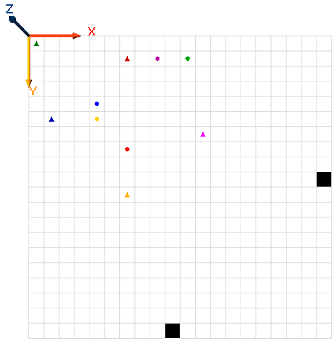
In order to demonstrate the performance of the affinity-based HetSRL method introduced in the last section, the shortest path problem from the start cell to targets in an by grid environment in considered here. Targets may be placed in arbitrary locations on the grid. Both targets and the agents are represented by a profile, i.e., an array of values, and the agents’ goal is to find the shortest path to the most relevant target. This problem resembles a recommendation system in which agents represent user preferences and try to predict the rating or preference a user would give to an item. This simulation considers a 30 by 30 environment, 10 agents with different profiles, and two different targets. Figure 1 illustrates the problem environment. Targets are located at (15,30) and (30,15), and the starting point is at (1,1), letting the coordinates at the top left be (1,1). Reaching the targets, an agent will receive a reward that is directly proportional to its affinity to the target, i.e., .
All the experiments were performed on Intel(R) Celeron(R) CPU 1.90GHz with 10 GB RAM on the Microsoft Windows 10 platform and the simulations have been conducted using the GAMA platform, which is a modeling and simulation development environment for building spatially explicit agent-based simulations [47].
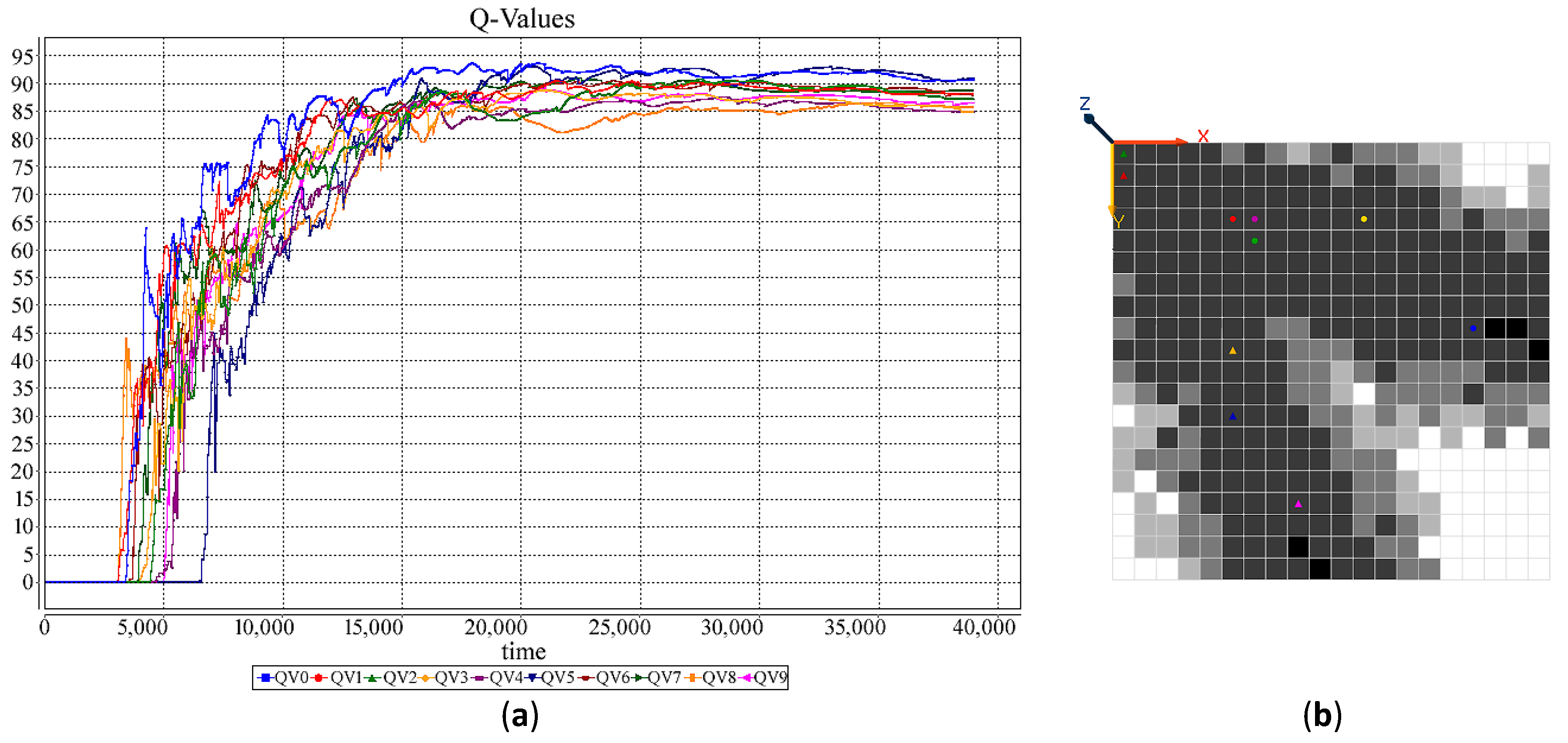
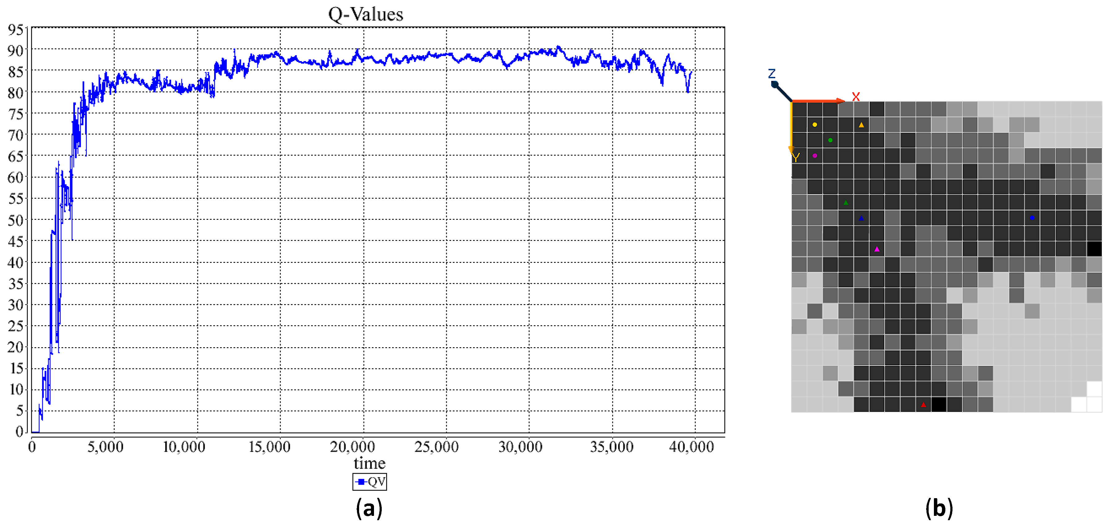
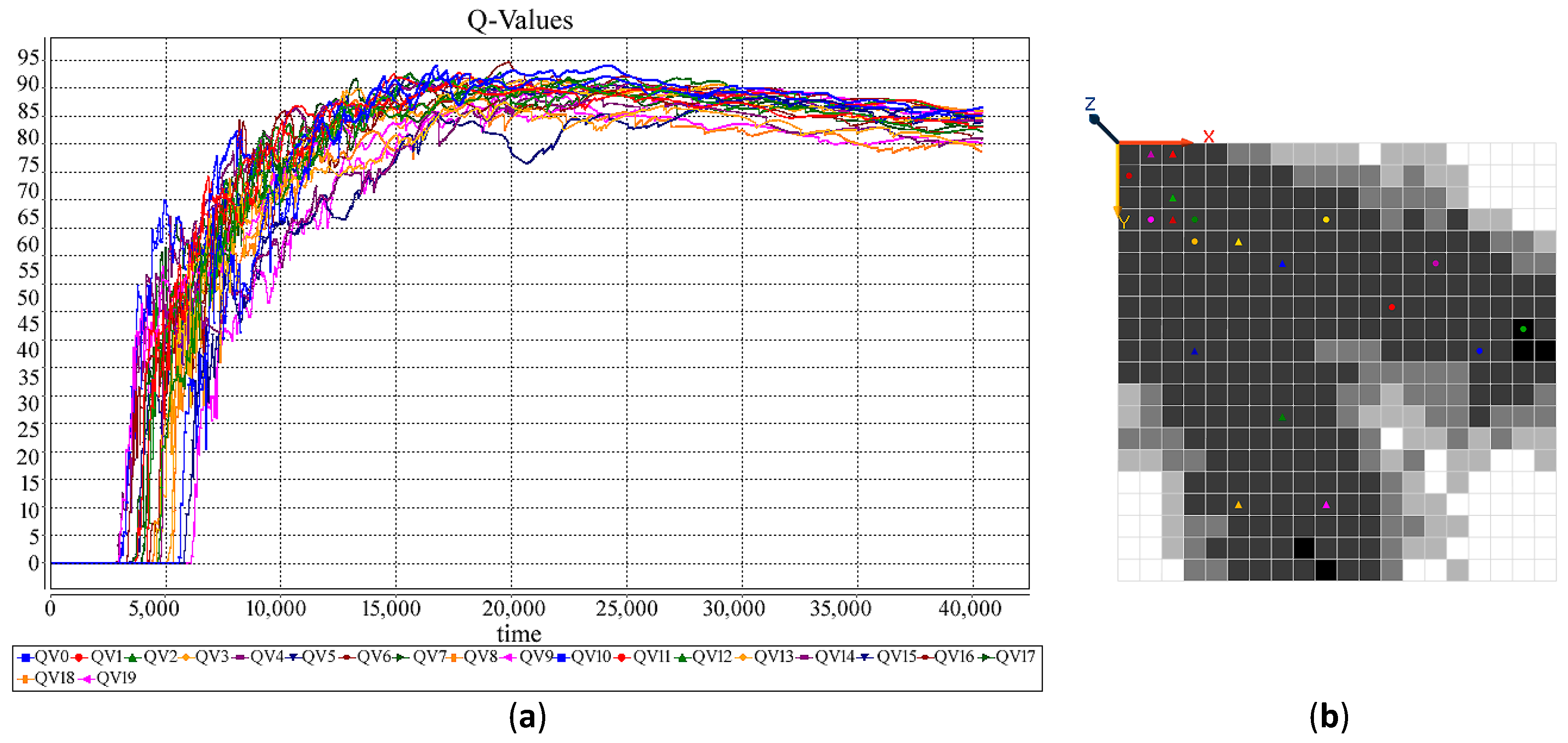
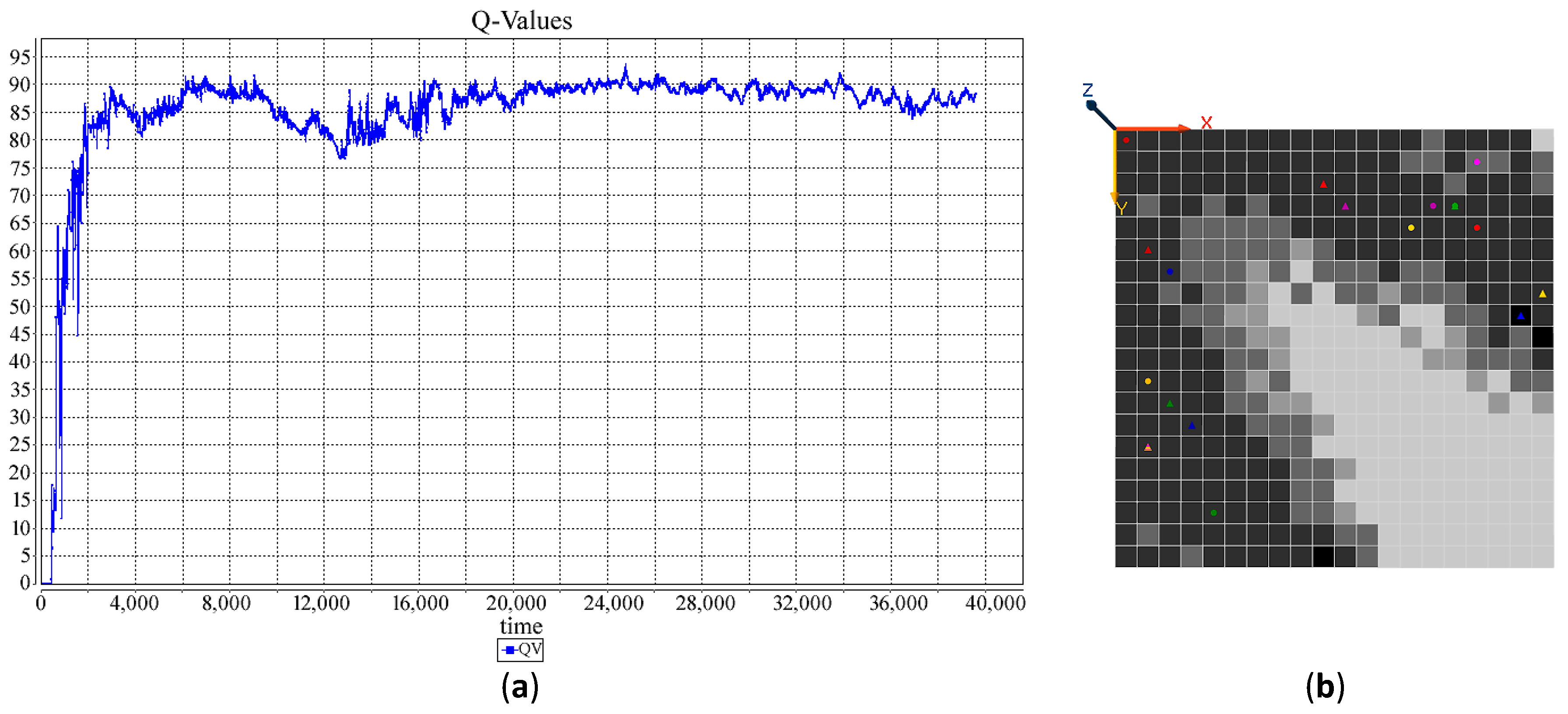
Figure 2, Figure 3, Figure 4 and Figure 5 demonstrate the changes of the Q-value at (1,1). Basically, the Q-Value remains zero until the first path from the starting point to a target is found, and the Q-value remain almost stable when the agent follows the almost the same path, i.e., the best found within a constraint timeframe, and has less intention to explore other possibilities.
Table 2 compares the approximate time of the first path detection and the approximate time needed for the optimal path detection for all of the four experiments. The results indicate that HetSRL has significantly reduced the search time, and the impact is more significant as the number of agents increases.
6. Holonic-Q-Learning: A Practical Application of the Affinity-Based HetSRL Method
This study aims to show how a carefully adapted HetSRL method can support a specific MAS, namely the Holonic Medical Diagnosis System (HMDS) in performing the self-organization process. In Section 6.1 the system and the relevant terms and concepts are introduced, Section 6.2 focuses on the affinity-based HetSRL method designed for this system, and Section 6.3 demonstrates the performance of this method.
6.1. The Holonic Medical Diagnosis System (HMDS)
The Holonic Medical Diagnosis System (HMDS) introduced in References [5,46], is a Holonic Multi-Agent System (HMAS) [48], which is capable of performing Differential Diagnosis (DDx). DDx is the distinguishing of a particular disease or condition from others presenting similar symptoms [49] that leads to more accurate diagnoses [50].
According to Reference [51], a holon is a natural or artificial structure that consists of several holons as sub-structures. A holonic agent of a well-defined software architecture may join several other holonic agents to form a super-holon; this group of agents, i.e., sub-holons, now act as if it were a single holonic agent with the same software architecture [48]. Depending on the level of observation, a holon can in fact be seen as an organization of holons or as an autonomous atomic entity, i.e., it is a whole-part construct, composed of other holons, but it is, at the same time, a component of a higher level holon [52].
The organizational structure of a holonic society, or holarchy, offers advantages that the monolithic design of most technical artifacts lack: They are robust in the face of external and internal disturbances and damages, they are efficient in their use of resources, and they can adapt to environment changes [48]. In fact, HMAS architecture confines the environment and accordingly the responsibility of the agents in different levels of holarchy. This will reduce the complexity of the system, ease the changes and hence speed up the convergence rate. Another attractive characteristic of HMASs is the support for self-organization, which is the autonomous continuous arrangement of the parts of a system in such a way that best matches its objectives. Obviously, all these advantages do not mean that HMAS architecture is more effective than the other architectures introduces for MASs, but specifically for the domains it is meant for.
As stated in Reference [48,53], domains suitable for holonic agents should involve actions that are recursively decomposable, exhibit hierarchical structures, and include cooperative elements. DDx domain meets the characteristics of holonic domain (see Reference [5]), and hence the HMDS is designed based on the holonic concepts.
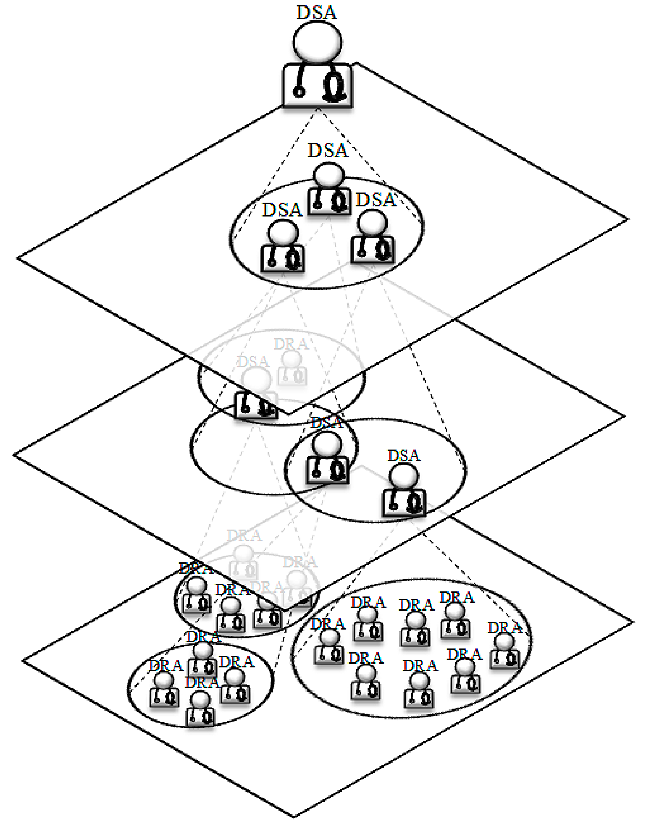
The HMDS consists of two types of agents: Comparatively simple Disease Representative Agents (DRA) as on the lowest level and more sophisticated Disease Specialist Agents (DSA) as decision makers on the higher levels of the system [46] (see Figure 6). DRAs are atomic agents and form the leaves of the holarchy. Each DRA is an expert on a specific disease and maintains the Disease Description Pattern (DDP)—an array of possible signs, symptoms, and test results, i.e., the holon identifier. In order to join the diagnosis process, these agents only need to perform some kind of pattern matching, i.e., calculating their Euclidean distance to the diagnosis request. DSAs are holons consisting of numbers of DRAs and/or DSAs with similar symptoms; i.e., representing similar diseases. This encapsulation, in fact, enables the implementation of the DDx. The DSAs are designed as moderated groups [48], where agents give up part of their autonomy to their super-holon. To this end, for each DSA, a head is defined, which provides an interface and represents the super-holon to its environment. This head is created for the lifetime of the super-holon, based on agent cloning. The holon identifier of a DSA will be the average of the holon identifiers of its members.
The holarchy has one root, i.e., a DSA, which will play the role of the exclusive interface to the outside world. Initially, this DSA takes all the DRAs as its members, and lets the DSAs form automatically. To this end, it clusters them based on the affinity, i.e., the similarity, and defines a head for each of the clusters. This is repeated recursively until no further clustering is necessary. Later on, the system can still reorganize its holarchy using its self-organization technique.
The HMDS works as follows: The head of the holarchy receives the diagnosis request and places it on its blackboard. Any member of this DSA can then read this message. A DRA’s reaction would be to send back its similarity to the request. However, a DSA will join the diagnosis process only if the request is not an outlier to its members. This means that it will place the diagnosis request on its own blackboard. Then the same process repeats recursively until the request reaches the final level of the holarchy. Results obtained by participating agents now flow from the bottom to the top of the holarchy and are sorted according to their similarity and frequency. Each agent will send its top diagnoses together with all of the signs, symptoms or test results that are relevant from its point of view, but their presence or absence has not been specified. This implies that originally not provided relevant information might be requested from the user in a second step [46]. For a more comprehensive description of the system and the demonstration of its functionality please refer to References [5,46].
6.2. Learning in HMDS
As mentioned above, the initial holarchy of the system can be created using clustering in different levels of the holarchy. Clustering is an unsupervised learning technique and hence doesn’t require any learning feedback. After having the initial holarchy, however, it is still essential to support the system in learning and updating based on the new observations. Medical knowledge demonstrates a steady upward growth, and diagnosis is also very much affected by the geographical regions. Hence, in order to adapt and improve the behavior of the system, we need to: (1) Update the medical knowledge based on the new instances, (2) reorganize the holarchy according to the experience and the feedback. In HMDS, holon identifiers are updated applying the exponential smoothing method, as a supervised learning method, and the self-organization of the holarchy is supported by Q-learning, as a reinforcement learning technique. Since both methods require feedback from the environment, it is clear that the quality of the feedback is of central importance. The rest of this section covers the above mentioned techniques and provides an experimental example, however, the discussion on the learning feedback can be followed in Reference [5].
The ML techniques being used in HMDS are:
Clustering: The Density-Based Spatial Clustering of Applications with Noise (DBSCAN) [54] is one of the best algorithms for clustering in HMDS. In [55] a simple and effective method for automatic detection of the input parameter of DBSCAN is presented, which helps best to deal with the complexity of the problem at hand.
Exponential Smoothing: Exponential smoothing is a very popular scheme for producing a smoothed time series [56]. Using this technique, the past observations are assigned exponentially decreasing weights and recent ones are given relatively higher weights:
where is the smoothing factor, and . As it is clear, the smoothed statistic is a simple weighted average of the current observation and the previous smoothed statistic . In HMDS, this method is used in order to update the holon identifiers.
Holonic-Q-Learning (HQL): The HMDS is a HetS, consisting of agents with different information and goals, which consequently leads to different behaviors. In this system, super-holons are mapping the sub-swarms. In contrast to the HetSs under consideration so far (see sec1, SI systems properties) the sub-swarms here are not homogeneous but again heterogeneous and may again include sub-swarms. Even though these sub-swarms are not homogeneous, the information and goals (behaviors) of their members are relatively more similar, such that they can exhibit swarm behavior. To this end, the degree of homogeneity, in our terminology the affinity between the agents, should be measured and considered.
The Holonic-QL is a Q-learning technique introduced for self-organization in the HMDS [46]. In HQL, the Q-value, in fact, measures how good it is for a holon to be a member (i.e., sub-holon), of another holon. In this case, the states are the existing holons and action indicates becoming a sub-holon of holon :
where,
and the reward is calculated by the head of a super-holon (see Reference [5]). For more information regarding the HQL and the proof of convergence please refer to Reference [46].
6.3. Simulation: A New DDx for Arthritis
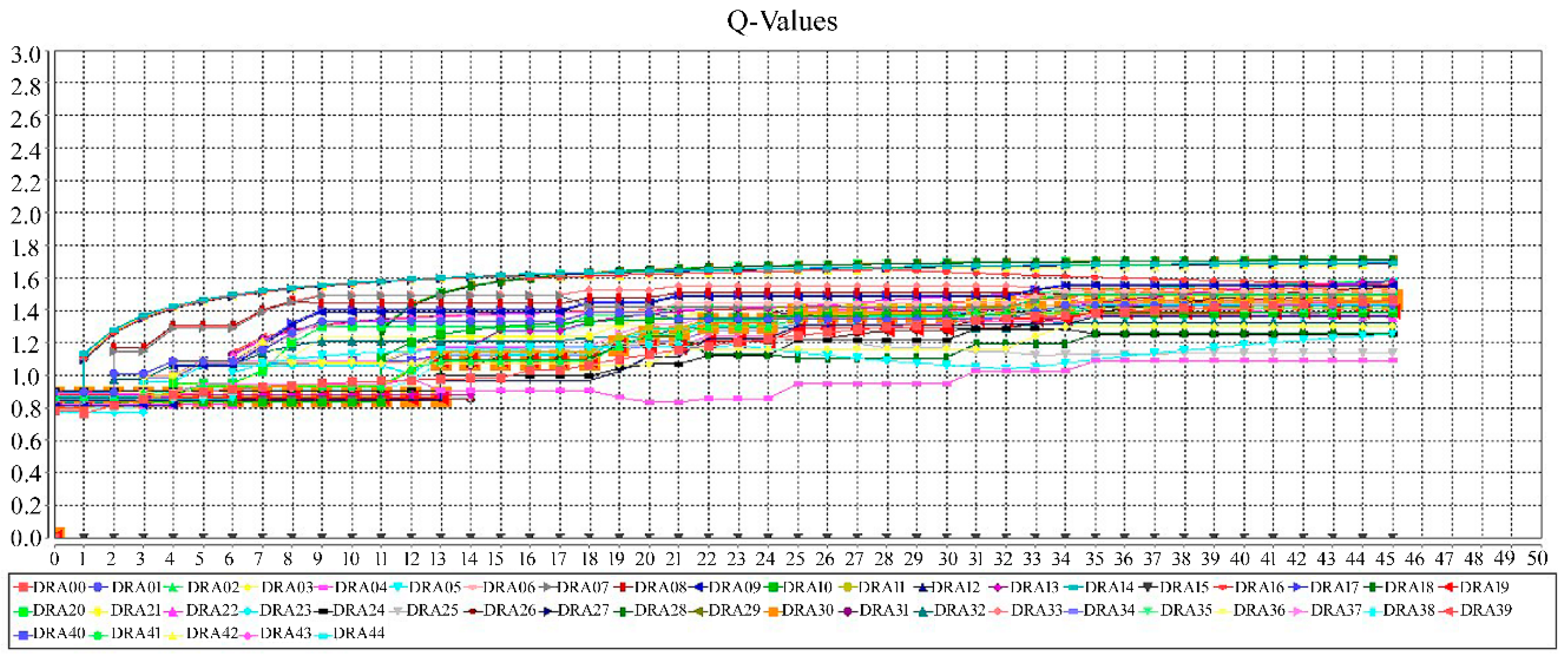
This section shows a simple simulation of the HMDS implemented using the GAMA platform [47]. The simulated system covers 45 diseases in a holarchy with four levels and the information regarding the diseases has been gathered from Mayo Clinic website [57], which provides detailed information about the diseases and their signs and symptoms. In order to check the state of the holarchy the Q-values of the DRAs are monitored on a chart. Figure 7 demonstrates the convergence of the Q-values of all 45 DRAs in the simulated system, which indicates that the holarchy is responsive and does not require any structural revisions, i.e., self-organization attempts, for the time being. An agent will consider to be an outlier with respect to the super-holon it is a member of if its Q-value is far away from the other members’ Q-values. In such case, this agent needs to explore and find a new super-holon considering its affinity to the new group.
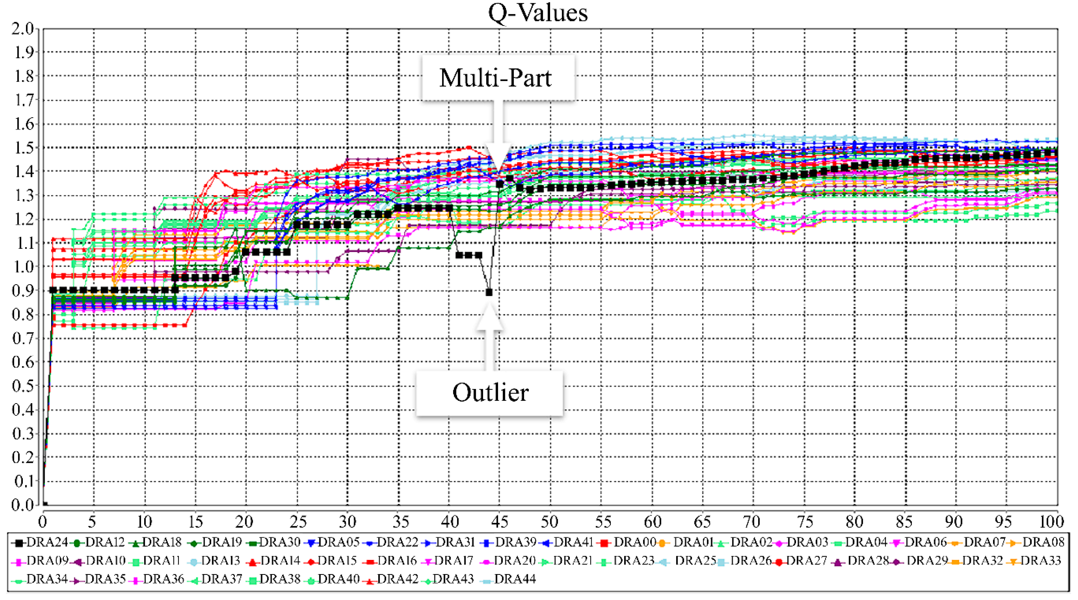
In this experiment a real medical case is used, in which the Madelung-Launois-Bensaude disease (MLB) is suggested as a new DDx for arthritis [58]. MLB is a disease that causes the concentration of fatty tissue in proximal upper body. In 2008, for the first time, some instances of this disease were observed with distal fatty tissue that were misdiagnosed first as arthritis, which normally includes joint pain and joint swelling. In this experiment, the new observations will be given to the HMDS, which so far does not consider the MLB disease with arthritis for the reason of DDx. The system should then be able to come to the same conclusion as in Reference [58] and add the DRA acting for the MLB disease to the super-holon containing the DRA acting for arthritis. Essentially, if an agent is not involved in a diagnosis process it will not receive any reward and hence its Q-value will remain same during that round. As the agent participates in a diagnosis process, it will be rewarded and hence its Q-value will be updated. In case the Q-value of any of the members of the super-holon is getting close to be a noise (close to lower three-sigma limit), the agent will start exploring new opportunities to join new super-holons. One promising approach for this agent is to try to become a member of those super-holons that were activated at the same time with its current super-holon. This will guarantee that the agent would have some common interests with the members of its new super-holon(s).
Figure 8 shows the changes in the Q-values of the different DRAs in the simulated case. Entering the distal MLB instances into the system, the Q-value of the DRA acting for the MLB disease will get closer to the lower outlier threshold. At this point, the super-holon of the arthritis disease will also be activated and as the DRA acting for the MLB disease is looking for a chance to join some new super-holons, it will be informed and will try to become a member of this super-holon. Considering the holon identifier of its members, this super-holon will then check whether the DRA acting for the MLB disease would be an outlier and since the case is negative, it will accept this new member. DRA acting for the MLB disease is now a Multi-Part (The “Part” role identifies members of a single holon. The “Multi-Part” role is an extension of the Part role and implies to a situation when a sub-holon is shared by more than one super-holon [52]). At this stage, the Q-value will be an accumulated value, calculated based on the rewards received from both super-holons. As it can be followed on the diagram, since this value is now greater than the average of the Q-values in both super-holons, the DRA acting for MLB will stop exploring at this point.
7. Conclusions
This study has introduced a novel affinity-based HetSRL Method that allows heterogeneous individuals to behave as a swarm in case they have identical sub-problems to solve. The affinity between two agents, i.e., the compatibility of agents to work together towards solving a specific sub-problem has been suggested to be measured and indicate the possibility of swarm behavior. As a result, the affinity-based HetSRL essentially allows the agents that are not identical but are capable of collaboration to exhibit swarm behavior providing them with the means of sharing their knowledge and eventually dealing with problems that match their specialties. This method basically allows such agents to gather information from a larger swarm and to be able to use this broader knowledge to make better decisions. The experiments have shown that this method is able to increase the performance of the heterogeneous agents solving SDMPs, however, it should be noted that the method is applicable when sub-groups with a significantly lesser extent of heterogeneity are extractable and are, in addition to that, populated sufficiently to be able to exhibit meaningful swarm behavior.
The idea of using a swarm of experts with similar specialties is indeed very similar to ensemble learning and particularly one of its commonly used algorithms, the mixture of experts. According to Reference [59], ensemble learning is the process by which multiple models, such as classifiers and experts, are strategically generated and combined to solve a computational intelligence problem. The mixture of experts algorithm [60] is one of the algorithms commonly used for ensemble learning that generates several experts whose outputs are combined through a generalized linear rule. A hierarchical mixture of experts can also be further combined if the output is conditional on multiple levels of probabilistic gating functions [61]. As a result, even though the usage of experts with similar specialties in the affinity-based HetSRL can be seen as an application of ensemble learning there is small but distinctive difference between these two approaches. In ensemble learning, experts are strategically generated differently to obtain better results than could be obtained from any of the constituent experts alone. In affinity-based HetSRL, however, heterogeneity is a feature of the agents of the environment and the idea is to provide those experts that can collaborate with each other with the means of sharing their knowledge and eventually dealing with problems that match their specialties.
Additionally, since applying the affinity-based HetSRL, the problem is modeled using a Markov chain and the heterogeneous agents can be seen as multi-labeled instances, it may be concluded that the problem can be modeled and solved using classifier chains, which is a machine learning method for problem transformation in multi-label classification [62]. The classifier chains method essentially builds a deterministic high order Markov chain model to capture the interdependencies between labels in multi-label classification problems [63]. However, classification cannot be used to build the Markov chain in the general problem environment that is under consideration in this study as neither the number of levels nor the number of the groups on each level are predefined. Classifier chains is a supervised learning approach, in which the desired input/output are provided, however, in reinforcement learning, the desired input/output pairs are not presented, and the algorithm estimates the optimal actions by interacting with a dynamic environment. As a result, reinforcement learning approaches are able to exhibit flexibility and are best used with open, dynamic, and complex environments.
Despite the promising results of this work in dealing with heterogeneous swarms, as most of the studies in the field of SI is concentrated on homogeneous swarms, it is highly recommended to address this knowledge gap thoroughly and increase the understanding of the constraints and the effective factors that should be taken into consideration when dealing with these swarms.
Author Contributions
Conceptualization, Z.A.; Methodology, Z.A.; Software, Z.A.; Validation, Z.A.; Formal Analysis, Z.A.; Investigation, Z.A.; Resources, Z.A.; Data Curation, Z.A.; Writing-Original Draft Preparation, Z.A.; Writing-Review & Editing, Z.A.; Visualization, Z.A.; Supervision, R.U.; Project Administration, R.U.
Funding
This research received no external funding.
Conflicts of Interest
The authors declare no conflict of interest.
References
- Puterman, M.L. Markov Decision Processes: Discrete Stochastic Dynamic Programming; John Wiley & Sons, Inc.: New York, NY, USA, 1994; p. 684. [Google Scholar]
- Littman, M.L. Algorithms for Sequential Decision Making. Ph.D. Thesis, Department of Computer Science, Brown University, Providence, RI, USA, 1996. [Google Scholar]
- Beni, G.; Wang, J. Swarm Intelligence in Cellular Robotic Systems. Robot. Biol. Syst. A New Bionics 1989, 102, 703–712. [Google Scholar] [CrossRef]
- Dorigo, M.; Floreano, D.; Gambardella, L.M.; Mondada, F.; Nolfi, S.; Baaboura, T.; Birattari, M.; Bonani, M.; Brambilla, M.; Brutschy, A.; et al. Swarmanoid: A novel concept for the study of heterogeneous robotic swarms. IEEE Robot. Autom. Mag. 2013, 20, 60–71. [Google Scholar] [CrossRef]
- Akbari, Z.; Unland, R. A Holonic Multi-Agent Based Diagnostic Decision Support System for Computer-Aided History and Physical Examination. In Proceedings of the Advances in Practical Applications of Agents, Multi-Agent Systems, and Complexity: The PAAMS Collection (PAAMS 2018), Lecture Notes in Computer Science, Toledo, Spain, 20–22 June 2018; Volume 10978, pp. 29–41. [Google Scholar]
- UNANIMOUS AI. Available online: https://unanimous.ai/ (accessed on 11 March 2019).
- Dorigo, M.; Birattari, M. Swarm intelligence. 2007. Available online: http://www.scholarpedia.org/article/Swarm_intelligence (accessed on 11 March 2019).
- Montes de Oca, M.A.; Pena, J.; Stützle, T.; Pinciroli, C.; Dorigo, M. Heterogeneous Particle Swarm Optimizers. In Proceedings of the IEEE Congress on Evolutionary Computation (CEC), Trondheim, Norway, 18–21 May 2009; pp. 698–705. [Google Scholar]
- Szwaykowska, K.; Romero, L.M.-y.-T.; Schwartz, I.B. Collective motions of heterogeneous swarms. IEEE Trans. Autom. Sci. Eng. 2015, 12, 810–818. [Google Scholar] [CrossRef]
- Ferante, E. A Control Architecture for a Heterogenous Swarm of Robots; Université Libre de Bruxelles: Brussels, Belgium, 2009. [Google Scholar]
- Kumar, M.; Garg, D.P.; Kumar, V. Segregation of heterogeneous units in a swarm of robotic agents. IEEE Trans. Autom. Control 2010, 55, 743–748. [Google Scholar] [CrossRef]
- Pinciroli, C.; O’Grady, R.; Christensen, A.L.; Dorigo, M. Coordinating heterogeneous swarms through minimal communication among homogeneous sub-swarms. In Proceedings of the International Conference on Swarm Intelligence, Brussels, Belgium, 8–10 September 2010; pp. 558–559. [Google Scholar]
- Engelbrecht, A.P. Heterogeneous particle swarm optimization. In Proceedings of the International Conference on Swarm Intelligence (ANTS 2010), Brussels, Belgium, 8–10 September 2010; pp. 191–202. [Google Scholar]
- Ma, X.; Sayama, H. Hierarchical heterogeneous particle swarm optimization: algorithms and evaluations. Intern. J. Parallel Emergent Distrib. Syst. 2015, 31, 504–516. [Google Scholar] [CrossRef]
- van Hasselt, H.P. Insights in Reonforcment Learning; Wöhrmann Print Service: Zutphen, The Netherlands, 2011; p. 278. [Google Scholar]
- Tandon, P.; Lam, S.; Shih, B.; Mehta, T.; Mitev, A.; Ong, Z. Quantum Robotics: A Primer on Current Science and Future Perspectives; Morgan & Claypool Publichers: San Rafael, CA, USA, 2017; p. 149. [Google Scholar]
- Sutton, R.S.; Barto, A.G. Reinforcement Learning: An Introduction; MIT Press: Cambridge, MA, USA, 1998; p. 322. [Google Scholar]
- Poole, D.; Mackworth, A. Artificial Intelligence: Foundations of Computational Agents; Cambridge University Press: New York, NY, USA, 2010; p. 682. [Google Scholar]
- Mitchell, T.M. Chapter 13: Reinforcement Learning. In Machine Learning; McGraw-Hill Science/Engineering/Math: New York, NY, USA, 1997. [Google Scholar]
- Vrancx, P. Decentralised Reinforcement Learning in Markov Games. Ph.D. Thesis, Vrije Universiteit Brussel, Brussels, Belgium, 2010. [Google Scholar]
- Coggen, M. Exploration and Exploitation in Reinforcement Learning; CRA-W DMP Project at McGrill University: Montreal, QC, Canada, 2004. [Google Scholar]
- Barto, A.G.; Sutton, R.S.; Anderson, C.W. Neuronlike adaptive elements that can solve difficult learning control problems. IEEE Trans. Syst. Man Cybern. 1983, SMC-13, 834–846. [Google Scholar] [CrossRef]
- Sutton, R.S. Learning to predict by the methods of temporal differences. Mach. Learn. 1988, 3, 9–44. [Google Scholar] [CrossRef] [Green Version]
- Watkins, C.J.C.H. Learning from delayed rewards. Ph.D. Thesis, Cambridge University, Cambridge, UK, 1989. [Google Scholar]
- Schwartz, A. A reinforcement learning method for maximizing undiscounted rewards. In Proceedings of the 10th International Conference on Machine Learning, Amherst, MA, USA, 27–29 July 1993; pp. 298–305. [Google Scholar]
- Rummery, G.A.; Niranjan, M. On-Line Q-Learning Using Connectionist Systems; Department of Engineering, University of Cambridge: Cambridge, UK, 1994; pp. 1–20. [Google Scholar]
- Wiering, M.A.; van Hasselt, H. Two novel on-policy reinforcement learning algortihms based on TD(λ)-methods. In Proceedings of the Approximate Dynamic Programming and Reinforcement Learning, ADPRL 2007, Honolulu, HI, USA, 1–5 April 2007. [Google Scholar]
- Hoffman, m.; Doucet, A.; de Freitas, N.; Jasra, A. Trans-dimensional MCMC for Bayesian Policy Learning. In Proceedings of the 20th International Conference on Neural Information Processing Systems, Vancouver, BC, Canada, 3–6 December 2007; pp. 665–672. [Google Scholar]
- Buşoniu, L.; Babuška, R.; Schutter, B.D. Multi-agent reinforcement learning: An overview. Innov. Multi-Agent Syst. Appl. 2010, 310, 183–221. [Google Scholar] [CrossRef]
- Tuyls, K.; Weiss, G. Multiagent Learning: Basics, Challenges, and Prospects. AI Mag. 2012, 33, 41–52. [Google Scholar] [CrossRef]
- Dorigo, M. Optimization, Learning and Natural Algorithms. Ph.D. Thesis, Politecnico di Milano, Milano, Italy, 1992. [Google Scholar]
- Gambardella, L.M.; Dorigo, M. Ant-Q: A Reinforcement Learning approach to the traveling salesmn problem. In Proceedings of the ML-95, 12th International Conference on Machine Learning, Tahoe City, CA, USA, 9–12 July 1995; pp. 252–260. [Google Scholar]
- Monekosso, N.; Remagnino, A.P. Phe-Q: A pheromone based Q-learning. In Proceedings of the Australian Joint Conference on Artificial Intelligence: AI 2001, LNAI 2256, Adelaide, SA, Australia, 10–14 December 2001; pp. 345–355. [Google Scholar]
- Iima, H.; Kuroe, Y.; Matsuda, S. Swarm reinforcement learning method based on ant colony optimization. In Proceedings of the 2010 IEEE International Conference on Systems Man and Cybernetics (SMC), Istanbul, Turkey, 10–13 October 2010; pp. 1726–1733. [Google Scholar]
- Hong, M.; Jung, J.J.; Camacho, D. GRSAT: A novel method on group recommendation by social affinity and trustworthiness. Cybern. Syst. 2017, 140–161. [Google Scholar] [CrossRef]
- Hong, M.; Jung, J.J.; Lee, M. Social Affinity-Based Group Recommender System. In Proceedings of the International Conference on Context-Aware Systems and Applications, Vung Tau, Vietnam, 26–27 November 2015; pp. 111–121. [Google Scholar]
- APA Dictionary of Psychology. Available online: https://dictionary.apa.org (accessed on 11 March 2019).
- Hill, C.; O’Hara O’Connor, E. A Cognitive Theory of Trust. 84 Wash. U. L. Rev. 2005, 84, 1717–1796. [Google Scholar] [CrossRef]
- Chatterjee, K.; Majumdar, R.; Henzinger, T.A. Markov decision processes with multiple objectives. In Proceedings of the Annual Symposium on Theoretical Aspects of Computer Science, Marseille, France, 23–25 February 2006; pp. 325–336. [Google Scholar]
- Lizotte, D.J.; Laber, E.B. Multi-Objective Markov Decision Processes for Data-Driven Decision Support. J. Mach. Learn. Res. 2016, 17, 1–28. [Google Scholar]
- Roijers, D.M.; Vamplew, P.; Whiteson, S.; Dazeley, R. A survey of multi-objective sequential decision-making. J. Artif. Intell. Res. 2013, 48, 67–113. [Google Scholar] [CrossRef]
- Hwang, C.-L.; Masud, A.S.M. Multiple Objective Decision Making, Methods and Application: A State-of-the-Art Survey; Springer: Berlin/Heidelberg, Germany, 1979; p. 351. [Google Scholar]
- Melo, F. Convergence of Q-learning: A simple proof; Institute Of Systems and Robotics, Tech. Rep (2001); Institute of Systems and Robotics: Lisbon, Portugal, 2001; pp. 1–4. [Google Scholar]
- Jaakkola, T.; Jordan, M.I.; Singh, S. Convergence of stochastic iterative dynamic programming algorithms. In Proceedings of the 6th International Conference on Neural Information Processing Systems, Denver, CO, USA, 29 November–2 December 1993; pp. 703–710. [Google Scholar]
- Jaakkola, T.; Jordan, M.I.; Singh, S. On the convergence of stochastic iterative dynamic programming algorithms. Neural Comput. 1994, 6, 1185–1201. [Google Scholar] [CrossRef]
- Akbari, Z.; Unland, R. A Holonic Multi-Agent System Approach to Differential Diagnosis. In Proceedings of the Multiagent System Technologies. MATES 2017, Leipzig, Germany, 23–26 August 2017; pp. 272–290. [Google Scholar]
- GAMA Platform. Available online: https://gama-platform.github.io/ (accessed on 11 March 2019).
- Gerber, C.; Siekmann, J.H.; Vierke, G. Holonic Multi-Agent Systems; DFKI-RR-99-03: Kaiserslautern, Germany, 1999. [Google Scholar]
- Merriam-Webster. Differential Diagnosis. Available online: https://www.merriam-webster.com/dictionary/differential%20diagnosis (accessed on 11 March 2019).
- Maude, J. Differential diagnosis: The key to reducing diagnosis error, measuring diagnosis and a mechanism to reduce healthcare costs. Diagnosis 2014, 1, 107–109. [Google Scholar] [CrossRef] [PubMed]
- Koestler, A. The Ghost in the Machine; Hutchinson: London, UK, 1967; p. 384. [Google Scholar]
- Rodriguez, S.A. From Analysis to Design of Holonic Multi-Agent Systems: A Framework, Methodological Guidelines and Applications. Ph.D. Thesis, University of Technology of Belfort-Montbéliard, Sevenans, France, 2005. [Google Scholar]
- Lavendelis, E.; Grundspenkis, J. Open holonic multi-agent architecture for intelligent tutoring system development. In Proceedings of the IADIS International Conference on Intelligent Systems and Agents, Amsterdam, The Netherlands, 22–24 July 2008. [Google Scholar]
- Ester, M.; Kriegel, H.-P.; Sander, J.; Xu, X. A Density-Based Algorithm for Discovering Clusters in Large Spatial Databases with Noise. In Proceedings of the 2nd International Conference on Knowledge Discoverey and Data Mining, Portland, OR, USA, 2–4 August 1996; pp. 226–231. [Google Scholar]
- Akbari, Z.; Unland, R. Automated Determination of the Input Parameter of the DBSCAN Based on Outlier Detection. In Proceedings of the Artificial Intelligence Applications and Innovations (AIAI 2016), IFIP Advances in Information and Communication Technology, Thessaloniki, Greece, 16–18 September 2016; Volume 475, pp. 280–291. [Google Scholar]
- NIST/SEMATECH e-Handbook of Statistical Methods. Available online: http://www.itl.nist.gov/div898/handbook/ (accessed on 11 March 2019).
- Mayo Clinic. Available online: https://www.mayoclinic.org/ (accessed on 11 March 2019).
- Lemaire, O.; Paul, C.; Zabraniecki, L. Distal Madelung-Launois-Bensaude disease: An unusual differential diagnosis of acromalic arthritis. Clin. Exp. Rheumatol. 2008, 26, 351–353. [Google Scholar] [PubMed]
- Polikar, R. Ensemble learning. 2009. Available online: http://www.scholarpedia.org/article/Ensemble_learning (accessed on 11 March 2019).
- Jacobs, R.A.; Jordan, M.I.; Nowlan, S.J.; Hinton, G.E. Adaptive mixtures of local experts. Neural Comput. 1991, 3, 79–87. [Google Scholar] [CrossRef]
- Jordan, M.I.; Jacobs, R.A. Hierarchical mixtures of experts and the EM algorithm. In Proceedings of the 1993 International Conference on Neural Networks (IJCNN-93-Nagoya, Japan), Nagoya, Japan, 25–29 October 1993; pp. 181–214. [Google Scholar]
- Read, J.; Pfahringer, B.; Holmes, G.; Frank, E. Classifier Chains for Multi-label Classification. In Proceedings of the 13th European Conference on Principles and Practice of Knowledge Discovery in Databases and the 20th European Conference on Machine Learning, Bled, Slovenia, 7–11 September 2009; pp. 254–269. [Google Scholar]
- Liu, W.; Tsang, I.W. On the optimality of classifier chain for multi-label classification. In Proceedings of the 28th International Conference on Neural Information Processing Systems, Montreal, QC, Canada, 7–12 December 2015; pp. 712–720. [Google Scholar]
Figure 1.
The problem environment.

Figure 2.
(a) Q-value chart for 10 single agents. (b) The amount of Q-Value for different cells.

Figure 3.
(a) Q-value chart for a Heterogeneous Swarm (HetS) with 10 agents. (b) The amount of Q-Value for different cells.
Figure 3.
(a) Q-value chart for a Heterogeneous Swarm (HetS) with 10 agents. (b) The amount of Q-Value for different cells.

Figure 4.
(a) Q-value chart for 20 single agents. (b) The amount of Q-Value for different cells.

Figure 5.
(a) Q-value chart for a Heterogeneous Swarm (HetS) with 20 agents. (b) The amount of Q-Value for different cells.
Figure 5.
(a) Q-value chart for a Heterogeneous Swarm (HetS) with 20 agents. (b) The amount of Q-Value for different cells.

Figure 6.
Disease Representative Agents (DRAs) and Disease Specialist Agents (DSAs) in The Holonic Medical Diagnosis System (HMDS).
Figure 6.
Disease Representative Agents (DRAs) and Disease Specialist Agents (DSAs) in The Holonic Medical Diagnosis System (HMDS).

Figure 7.
The convergence of the Q-Values of the different Disease Representative Agents (DRAs) in the Holonic Medical Diagnosis System (HMDS).
Figure 7.
The convergence of the Q-Values of the different Disease Representative Agents (DRAs) in the Holonic Medical Diagnosis System (HMDS).

Figure 8.
The changes in the Q-values of the different Disease Representative Agents (DRAs) in the simulated case.
Figure 8.
The changes in the Q-values of the different Disease Representative Agents (DRAs) in the simulated case.


Table 1.
The notable reinforcement learning techniques.
| RL Technique | Policy | Year | Reference |
|---|---|---|---|
| Actor-Critic (AC) | on-policy | 1983 | [22] |
| Temporal Difference (TD) | on-policy | 1988 | [23] |
| Q-Learning | off-policy | 1989 | [24] |
| R-Learning | off-policy | 1993 | [25] |
| State-Action-Reward-State-Action (SARSA) | on-policy | 1994 | [26] |
| Actor Critic Learning Automaton (ACLA) | on-policy | 2007 | [27] |
| QV(λ)-Learning | on-policy | 2007 | [27] |
| Monte Carlo (MC) for RL | on-policy | 2008 | [28] |
© 2019 by the authors. Licensee MDPI, Basel, Switzerland. This article is an open access article distributed under the terms and conditions of the Creative Commons Attribution (CC BY) license (http://creativecommons.org/licenses/by/4.0/).
Share and Cite
MDPI and ACS Style
Akbari, Z.; Unland, R. A Novel Heterogeneous Swarm Reinforcement Learning Method for Sequential Decision Making Problems. Mach. Learn. Knowl. Extr. 2019, 1, 590-610. https://doi.org/10.3390/make1020035
AMA Style
Akbari Z, Unland R. A Novel Heterogeneous Swarm Reinforcement Learning Method for Sequential Decision Making Problems. Machine Learning and Knowledge Extraction. 2019; 1(2):590-610. https://doi.org/10.3390/make1020035
Chicago/Turabian StyleAkbari, Zohreh, and Rainer Unland. 2019. "A Novel Heterogeneous Swarm Reinforcement Learning Method for Sequential Decision Making Problems" Machine Learning and Knowledge Extraction 1, no. 2: 590-610. https://doi.org/10.3390/make1020035