Abstract
Dimensionality reduction methods can be used to project high-dimensional data into low-dimensional space. If the output space is restricted to two dimensions, the result is a scatter plot whose goal is to present insightful visualizations of distance- and density-based structures. The topological invariance of dimension indicates that the two-dimensional similarities in the scatter plot cannot coercively represent high-dimensional distances. In praxis, projections of several datasets with distance- and density-based structures show a misleading interpretation of the underlying structures. The examples outline that the evaluation of projections remains essential. Here, 19 unsupervised quality measurements (QM) are grouped into semantic classes with the aid of graph theory. We use three representative benchmark datasets to show that QMs fail to evaluate the projections of straightforward structures when common methods such as Principal Component Analysis (PCA), Uniform Manifold Approximation projection, or t-distributed stochastic neighbor embedding (t-SNE) are applied. This work shows that unsupervised QMs are biased towards assumed underlying structures. Based on insights gained from graph theory, we propose a new quality measurement called the Gabriel Classification Error (GCE). This work demonstrates that GCE can make an unbiased evaluation of projections. The GCE is accessible within the R package DR quality available on CRAN.
1. Introduction
Dimensionality reduction techniques reduce the dimensions of the data and try to preserve meaningful similarities in the low-dimensional space. DR can be used to facilitate the exploration of such structures in high-dimensional data by projecting the data into two-dimensional space.
This work focuses on the evaluation of two-dimensional projections of high-dimensional data, intending to select the projection that represents relevant high-dimensional similarities appropriate. A valid visualization of high-dimensional information is possible if a projection method can retain the structures of high-dimensional data in the two-dimensional space. For example, such a two-dimensional scatter plot remains a state-of-the-art form of visualization used in cluster analysis (e.g., [1,2,3,4]).
However, the consequence of limiting the output space to two dimensions is that the low-dimensional similarities cannot completely represent the high-dimensional similarities, which can result in a misleading interpretation of the underlying structures; One solution is to evaluate such structures using quality measurements (QMs). Consequently, QMs should be able to assess two-dimensional visualizations of high-dimensional data. High-dimensional structures can be either linear or nonlinear separable through either distance or density.
To date, QMs have mostly been applied to datasets with a continuous structure such as a Swiss roll shape [5,6], an s-shape [7], or a sphere [8], for which the challenge is to represent the structure in two dimensions visually.
Gracia et al. [9] illustrate the other common evaluation approach: using various high-dimensional datasets for which prior classifications are available. The authors of [9] conducted a study on several QMs based on 12 real-world datasets analyzing the correlations between the QMs. However, they did not investigate whether the classification matched separable structures or the prior knowledge of a domain expert. Instead of evaluating QMs, Ray et al. [10] assessed with accuracy and F1 score the performance of classical classifiers after DR methods were used for feature selection or extraction. Ayesha et al. used an EEG dataset with 188 dimensions and 1,094,446 cases to compare various DR methods visually [11]. Whether these datasets possess any kind of separable structures independent of the classification was not discussed. Whether these datasets possess any kind of separable structures independent of the classification was not discussed.
This work seeks to achieve the following:
- Theoretical comparison with prior works about quality measurement of DR methods reveals biases that can be aggregated into semantic classes.
- Hence, a new open-source available quality measure called Gabriel classification error (GCE) is proposed for investigating the quality of DR methods given prior knowledge about a dataset.
- The overall value yielded by GCE ranks projections more intuitively, choosing projections with a higher class-based structure separation above others.
- GCE can be visualized as an error per point, providing the user a focus on the critical areas of the projection of the DR method.
- Using three datasets, GCE is compared to prior works.
The first step in assessing the performance of the two-dimensional visualizations provided by DR methods is to assess the methodology behind the QMs. Section 2 introduces the necessary mathematical definitions for understanding the general concept of neighborhoods based on graph theory. Section 3.1 and Appendix A provide a literature review of existing QMs. Section 3.2. presents the semantic categorization implied by the mathematical definitions stated in Section 2 and Section 3.1, and Appendix A. Section 4 introduces our new proposed QM. Overall, 19 QMs are categorized into semantic groups based on a neighborhood concept, and their advantages and limitations will become visible in the results section (Section 5). We will illustrate biases of QMs on artificial (Section 5.1 and Section 5.2) and real-world, high-dimensional datasets (Section 5.3). The discussion (Section 6) will evaluate the findings of the results in depth, focusing on the definition of the QMs, the structures which are priorly defined for the artificial datasets, the decisions required by the user, and the computational complexity of the QMs. The conclusion (Section 7) shortly summarizes the findings. Figure 1 shows the experimental plan, illustrating the datasets, the respective applied DR techniques and the various resulting tabulated scalar values of the QMs and the visualizations which are mandatory for some QMs.
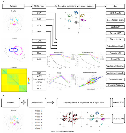
Figure 1.
The framework of the analysis performed in this work for dimensionality reduction. On three exemplary datasets, the shown projection methods are applied. Thereafter the projections onto a two-dimensional plane are evaluated with the displayed quality measurements in (A). The selection of quality measurements is based on theoretical analysis and available source code. In (B), the alternative evaluation of dimensionality reduction methods is proposed using the Gabriel classification error (GCE). It can either be visualized per point or an overall value can be provided.
2. Generalization of Neighbourhoods
We propose to use shortest paths and graph-based direct adjacency to generalize the neighborhoods H of an extent k as follows:
2.1. Graph Metrics
Let , let be a connected (weighted) graph with vertex set contained in a metric space . We will call points in data points. Let be a point in and let be the (weighted) graph distance of and an arbitrary point i.e., letting denote the sum of weights of edges of a path in we set
If for no explicit weights are given we choose to weight the edges as and so obtain as the length of and for the length of the shortest path connecting and .
In order to model discrete proximity, we rank distances from , i.e., let be all possible graph distances from , , in ascending order. If for given we have we write .
The set of neighbors of rank is then given as:
and defines a neighborhood set around . We say is the extent of this neighborhood. The neighborhood can define a pattern in the input space . The easiest example is a neighborhood defined by distances in a Euclidean graph. In the context of graph theory, a Euclidean graph is an undirected, weighted complete graph. Note that the weights of the vertices in a Euclidean graph need not necessarily be defined by the Euclidean metric. They are commonly inferred from the distance of the vertices in the ambient space The Euclidean graph is the only weighted graph considered. All subgraphs are thus viewed as having trivial weights.
Another setting for this definition is a Delaunay graph , which is a subgraph of a Euclidean graph. A Delaunay graph is based on Voronoi cells [12]. Each cell is assigned to one data point and is characterized in terms of the points in ambient space nearest to this particular data point. Within the borders of one Voronoi cell, there is no point that is nearer to any data point other than the data point within the cell. Thus in this setting, the neighborhood of data points is defined in terms of shared borders of Voronoi cells that induce an edge in the corresponding Delaunay graph [13]. We will denote the neighborhoods generated in this way by .
Yet another setting is the case of a Gabriel graph [14], which is a subgraph of a Delaunay graph in which two points are connected if the line segment between the two points is the diameter of a closed disc that contains no other data points within it (empty ball condition). The corresponding neighborhood will be called .
Lastly, an often-considered example is that of a neighborhood where the number of nearest neighbors of a data point is defined by the number of vertices connected to this point in the -nearest-neighbor graph (KNN graph) , e.g., [15]. Here, we will use the shorthand notation .
Neighborhoods of points can be divided into two types, namely, unidirectional and direction-based neighborhoods. Consider the four points shown in Figure 2. The points , and are in the same neighborhood ) in the corresponding Delaunay graph, but the points and are never neighbors in this graph, even if the distance is smaller than . Thus, in this neighborhood definition, the direction information is more important than the actual distance of the points in ambient space.
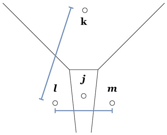
Figure 2.
Four points l, k, and m and their Voronoi cells. The distance between l and k is larger than between l and m: . Between l and m lies the point j. The example illustrate the different types of neighborhoods: unidirectional versus direction-based.
However, if we consider the setting where a neighborhood is defined in terms of the KNN graph, the points and could be neighboring ) while the points and could be non-neighboring, depending on the value of and on the ranking of the distances between these points. Therefore, this type of neighborhood is called unidirectional. In other words, it can be said that the points , and are denser with respect to each other than they are with respect to . Thus, unidirectional neighborhoods defined in terms of KNN graphs or unit disk graphs [16] can be used to define neighborhoods based on density.
2.2. Structure Preservation
Suppose that there exists a pair of similar high-dimensional data points such that . For visualization, the goal of a projection is to match these points to the low-dimensional space ; e.g., data points in close proximity should remain in close proximity, and remote data points should stay in remote positions. We will denote the image of in by for now and let denote the output space, i.e., the image of under this mapping. Further, let be the graph generated on in the same way as was obtained from .
Consequently, two kinds of errors exist. The first is forward projection error (FPE), which occurs when similar data points are mapped onto far-separated points:
for some .
The second is backward projection error (BPE), which occurs when a pair of closely neighboring positions represents a pair of distant data points:
for some .
It should be noted that similar definitions are found in [17] for the case of a Euclidean graph; in [8], for the case of a KNN graph of binary neighborhood, where BPE and FPE are referred to as precision and recall, respectively, and in [18], for the case of a Delaunay graph, where BPE and FPE are referred to as manifold stretching and manifold compression, respectively.
However, the FPE and BPE are not sufficient measurements for evaluating projections if the goal is to estimate the number of clusters or to ensure a sound clustering of the data [19]. In such a case, a suitable DR method should be able to also preserve nonlinear separable structures, i.e., regions in which values of the estimated probability density function tends towards zero. Such gaps should allow a DR method to distinct structures, meaning they should be projected in separate areas on the two-dimensional plane. For example, data lying on a hull encompassing a compact core will yield BPE/FPEs in every DR method that projects it onto a two-dimensional surface. While distances or even all neighborhoods may not be preserved in two dimensions, it is possible to preserve the two structures because of their distinction in the probability density function. If the DR method cannot account for sparse regions, for example, if data from different classes is cluttered with low density, the projection should at least show such cases as outliers or outstanding patterns. Vividly, structures divide a dataset in the input space I into several clusters of similar elements represented by points. However, the DR method should not visualize structures in two dimensions that do not exist in the high-dimensional space [20].
3. Quality Measurements (QMs)
In this section, the well-known measurements for assessing the quality of projections are introduced in alphabetical order. Some QMs use the ranks of distances instead of the actual distances between points. In this case, the following shorthand notation will be used:
Let be an entry in the matrix of the distances between all N points in a metric space M, where ; then, the rank denotes the position in the consecutive sequence of all entries of this matrix arranged in value from smallest to greatest. In short, the ranks of the distances are the relative positions of the distances, where R denotes the ranks of the distances in the input space and r denotes the ranks of the distances in the output space. Occasionally, ranks are represented by a vector in which the entries are the ranks of the distances between one specific point and all other points. Typically, the matrix or vector of ranks is normalized such that the values of its entries lie between zero and one.
3.1. Common Quality Measurements
3.1.1. Classification Error (CE)
This type of error is often used to compare projection methods when a prior classification is given [5,8,9,21].
Each point in the output space is classified by a majority vote among its k-nearest neighbors in the visualization [8], although sometimes simply the cluster of the nearest neighbor is chosen. This classification is compared with the prior classification as follows: Let denote the classification of the points in the input space, where denotes a cluster of the classification in I. Let denote the projected points in the output space that map to I. Let be the neighborhood of in a KNN graph in the output space. Then, the clusters are sorted, and the clusters with the largest number of points are chosen:
If , then
The label is then compared with . This yields the error:
3.1.2. C Measure
The C measure is a product of the input and output spaces in terms of similarity functions [22]. For ease of comparison, in Equation (8), the similarity function is redefined as the distance between two points. Consequently, the C measure is defined based on a Euclidean graph.
In the equation below, C is replaced with the capital letter F:
Since the error measure is not invariant under scaling of the output space O we cannot relate different F values for different projections. In order to compensate for this flaw the minimal path length is introduced. It tries to solve this issue by removing the weighting of D by d and instead only uses the ranks induced by d. In particular, it is minimal if the k-neighborhoods of I and O match.
3.1.3. Two Variants of the C Measure: Minimal Path Length and Minimal Wiring
Equation (6) presents the definition of the minimal path length [23], and Equation (7) defines the minimal wiring [24]:
where Equation (8) with defines the k nearest neighbors. Thus, it is analogous to a KNN graph:
where in Equation (6), M = I to define the set of the nearest spatial neighbors in the input space I, and in Equation (7), to serve the same purpose for the output space. A smaller value of the error F indicates a better projection.
3.1.4. Precision and Recall
Refs. [8,17] are based on the following concept: Venna et al. [8] defined misses as similar data points ∈ that are mapped to far-separated points ∈. Conversely, if a pair of closely neighboring positions represents a pair of distant data points, then this pair is called a false positive. From the information retrieval perspective, this approach allows one to define the precision and recall for cases where the neighborhoods are merely binary. However, [8] goes a step further by replacing such binary neighborhoods with probabilistic ones loosely inspired by stochastic neighbor embedding [25]. The neighborhood of the point l is defined with respect to the relevance of the points around l:
where is set to the value for which the entropy of is equal to log(knn) and knn is a rough upper limit on the number of relevant neighbors and is set by the user [8]. The authors propose a default value of 20 effective nearest neighbors. Similarly, the corresponding neighborhood in the output space is defined as:
These neighborhoods are compared based on the Kullback–Leibler divergence (KLD). Applying Equations (9) and (10), KLD is used to define the precision and recall :
The precision and recall (P&R) are plotted using a receiver operating characteristic (ROC)-like approach, in which the negative definition of the values results in the best projection method being displayed in the top right corner. For simplicity, we evaluate here the positive values meaning that higher values will indicate a lower structure preservation. The authors call these measurements smoothed because P&R are not normalized, and they also propose a normalized version, with values lying between zero and one, based on ranks instead of distances. Note that the KLD and the symmetric KLD do not follow the triangle inequality for metric spaces. This means that detours in the high-dimensional space compared to the direct edge between data points in the Euclidean graph, do not necessarily increase the distance. The violation of the triangular inequality could lead to inconsistent comparisons between points in the low-dimensional space in terms of similarity.
3.1.5. Rescaled Average Agreement Rate (RAAR)
The average agreement rate is defined in Equation (13) as:
in [26], analogously to the LCMC, using the unified co-ranking framework [27], in which the T&D, MRRE, and LCMC measurements can all be summarized mathematically (for further details, see [28]). Lee et al. [26] argue to enable fair comparisons or combinations of values of Q(knn) for different neighborhood sizes, the measurement in Equation (13) must be rescaled to:
This quantity is called the rescaled average agreement rate (RAAR). In Equations (13) and (14), knn is the abbreviation for the k-nearest neighbors and defines the size of the neighborhoods used in the formula. The error F is typically computed for a range of knn and visualized as a functional profile. The values of F lie in the interval between zero and one, with a logarithmic knn scale and a scalar value that can be obtained by calculating the area under the curve (AUC).
3.1.6. Stress and the Shepard Diagram
The original multidimensional scaling (MDS) measure has various limitations, such as difficulties with handling non-linearities (see [29] for a review); moreover, the underlying metric must be Euclidean, and Sammon Mapping is a normalized version of MDS. Therefore, only non-metric MDS is considered here. The calculated evaluation measurement is known as the stress and was first introduced in [30]. Here, the stress F is defined as shown in Equation (15). The disparities are the target values for each , meaning that if the distances in the output space achieve these values, then the ordering of the distances is preserved between the input and output spaces [22].
The input-space distances are used to define this measurement based on a Euclidean graph. Several algorithms exist for calculating . Kruskal [31] regarded F as a sort of residual sum of squares. A smaller value of F indicates a better fit. Therefore, perfect neighborhood preservation is achieved when F is equal to zero [31].
3.1.7. Trustworthiness and Discontinuity (T&D)
Venna and Kaski [32] introduced the T&D measurements, namely, trustworthiness and discontinuity. For ease of notation, we identify with its corresponding set of points in and analogously with its corresponding set of points in . Thus, denotes the set of points being -nearest neighbors of but coming from a point not being a -nearest neighbor of . Similarly is the set of points with being a -nearest neighbor of but being projected to a point not being a -nearest neighbor of . Note how this is related to the idea of FPE and BPE. Furthermore, let and denote the distance ranks in and , respectively. Then, the T&D are defined as:
where is a normalization constant depending on the dimension of the input space ambient to and the parameter mapping and to [0, 1], c.f. [33] is the trustworthiness (T), and is the discontinuity (D). By counting the number of intruders, the T&D measurements quantify the difference in the overlap of rank-based neighborhoods in I and O: represents the number of points that are incorrectly included in the input-space neighborhood, and represents the number of points that are incorrectly ejected from the input-space neighborhood.
Venna and Kaski claim that the trustworthiness () quantifies from “how far from the original neighborhood [in the input space I the new points [] entering the [output-space] neighborhood [H(knn, O/I)] come” [32]. For the calculation of the T&D measurements, KNN graphs must be generated for various knn values. Then, the trend of the curve can be interpreted. It is unclear how many knn values must be considered. Hence, knn values up to 25% of the total number of points are plotted. Lee and Verleysen showed that the T&D measurements can be expressed as a special case of the co-ranking matrix [28].
The authors consider a projection onto a display trustworthy if all samples close to each other after the projection can also be trusted to have been proximate in the original space [33]. Discontinuities in the projection are measured by how well neighborhoods of data points in the input space were preserved [33]. In terms of this work, the former minimizes the forward projection error (FPE) and the latter, the backward projection error (BPE in the case that proximation is defined in terms of the knn graph). However, the trade-off between trustworthiness and discontinuity is difficult to set as elaborated in Section 2.2. Structure Preservation. The choice of the knn values depends on the dataset. If sufficient prior knowledge about the data is given or can be extracted from the data utilizing knowledge discovery, it is possible to select an appropriate value for the knn.
3.1.8. Overall Correlations: Topological Index (TI) and Topological Correlation (TC)
Various applications of the two correlation measurements introduced below can be found in the literature.
The first type of correlation was introduced in [34] as Spearman’s and, in the context of metric topology preservation, was renamed as the topological index (TI) in [35]; see [36] for further details. In Equation (18), we follow the definition of the TI given in [36], with , where n is the number of distances:
The values of the TI are between zero and one, but [22] argued that the values of Spearman’s depend on the dimensions of the input and output spaces. Moreover, research has indicated that the elementary Spearman’s does not yield proper results for topology preservation [37].
In principle, correlations measure the preservation of all distances. Spearman correlation restricts the preservation to the ranks of distances. Instead of computing ranks of distances, topological correlation restricts the preservation of distances to Delaunay paths. In contrast to Kendall’s tau, all three approaches measure linear relationships [38,39]:
where and are the means of the entries in the lower half of the distance matrices and , with n being the number of distances. The TC is preferable to the TI as a means of characterizing topology preservation because in the case of the TI, the matching of extreme distances is sufficient to yield reasonably high overall correlation values [38].
3.1.9. Zrehen’s Measure
Zrehen’s measure operates on the empty ball condition of the Gabriel graph [14]. The neighborhood of each pair of projected points in the output space is depicted using locally organized cells:
“A pair of neighbor cells A and B is locally organized if the straight line joining their weight vectors W(A) and W(B) contains points which are closer to W(A) or W(B) than they are to any other” [40].
In this work, the strong connection between the TF value and the measurements called Zrehen [41] is remarked, but in contrast to [40], who assumed a neural net in two dimensions with precisely defined neighborhoods, here the output-space neighborhood is generalized to a Gabriel graph representation. Furthermore, for each pair of nearest neighbors, the TF considers the neighborhood order h for that pair, whereas [40] counts the number of intruding points in neighborhoods of all orders h (for details, see the section on the TF above).
In summary, if the condition is met, then all points that lie between the corresponding points and in are deemed intruders and are counted. For example, take and immediately adjacent in the output space and the corresponding data points and in the input space, then in the red circle, no further point of the data space should occur, as Figure 3 shows.
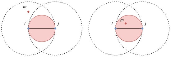
Figure 3.
Empty ball condition of the Gabriel graph. (Left): m is an intruder. (Right): m is no intruder.
The sum of the number of intruders for all pairs of neighbors is normalized using a factor that depends only on the size and topology [40]:
If let
And if . To allow for a clearer comparison between datasets, we set the error F as
where N is the number of data points. The range of F starts at zero and extends to positive infinity, with a value of zero indicating the best possible projection.
3.2. Types of Quality Measurements (QMs) for Assessing Structure Preservation
In general, three types of QMs and some special cases can be identified, as shown in Figure 4. The first type of QMs is called compact because measurement of this type compares the arrangement of all given points in the metric space as expressed in terms of distance. In the literature, the term topographic is often used for such QMs, e.g., [22]. These QMs depend on some kind of comparison between inter- and intra-cluster distances.
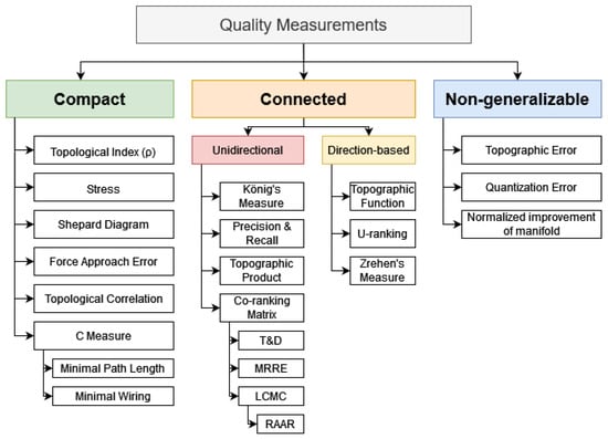
Figure 4.
Semantic groups of quality measurements (QMs). The “Compact” semantic class measures the preservation of distances, usually under the assumption that convex hulls of structures do not overlap, i.e., the structures are linear separable. The “Connected” semantic class restricts quality measurements to a neighborhood concept based on a specific graph. If an appropriate neighborhood concept is selected, the preservation of linear non-separable structures can be evaluated. For direct versus unidirectional structure concepts, we refer to Figure 2. The SOM-based class consists of QMs that require weights of neurons (prototypes) and therefore are not generalizable to every projection method. Abbreviations: trustworthiness and discontinuity (T&D), mean relative rank error (MRRE), local continuity meta-criterion (LCMC), and rescaled average agreement rate (RAAR).
QMs in the second group are based on a neighborhood definition and are called connected. These QMs rely on a type of predefined neighborhood H based on graph theory with a varying neighborhood extent k; thus, these neighborhoods are denoted by . The expression topology preservation is often used in reference to this type of QMs, e.g., [36]. The special cases are grouped together under the term non-generalizable QMs. These QMs, for example, the quantization error [42], the topographic error [43], or the normalized improvement of the manifold [44], are not considered any further here. Both quantization and topographic errors require calculations of the distances between the data points in the input space and the weights of the neurons (prototypes) in the output space in an SOM. Instead of prototypes, general projection methods consider projected points, which can also refer to the positions of neurons on a lattice. Distances between spaces of unequal dimensions are not mathematically defined. Several high-quality reviews are available on the subject of measuring SOM quality [41,45,46]. In the case of normalized improvement of the manifold, the QM requires a definition of eigenvectors typically not given for non-linear DR methods (e.g., [41,42,43,45,46,47]).
The neighborhood-based QMs are divided into two groups, called unidirectional QMs and direction-based QMs. The reason for this is that two points (j, k) that lie in the same direct neighborhood of point l in ) may not lie in the same neighborhood ) in the KNN graph if the distance D(l, k) is greater than the distance D(l, m) for a point m behind point j (see Figure 2 and Section 2.2).
4. Introducing the Gabriel Classification Error
For a data point, let be its classification, and for a given classification let be the set of data points with classification . Let and be the projected points in the output space that are mapped to I and let be the direct neighborhood of in the Gabriel graph of in the output space. Then, the neighboring points of are ranked using the Euclidean input-space distances between and ; i.e., let be indexed such that for in the Euclidean ambient space, it holds that Then let
where the number of nearest neighbors considered is a fixed parameter:
We say that and are falsely neighboring (for a given value of ) if
but .
The false neighbors of can thus be counted as:
Let denote the size of and denote the maximum for the GCE measurement is defined as:
A low GCE value indicates a structure-preserving projection in the sense that neighboring points of the Gabriel graph in the output space coming from close points in the input space have the same classification. Note that the GCE can be simplified to:
where is the matrix whose columns are:
for and
Furthermore, is an matrix with the following definition: Let
be the distance matrix of multiplied component-wise by the adjacency matrix of the Gabriel graph, where this adjacency matrix is defined as:
Let be the matrix where the entries in every row are sorted in ascending order; let be the reordering applied to the -th column of in this process (i.e., is the index of the -th nearest neighbor of in ). We set the elements of the matrix as:
Note that assigns the heaviest weights to the errors that are nearest to a given point. The range of the GCE is and thus raw GCE favors projections with Gabriel graphs having small neighborhoods; however, in order to compare projections independent of this bias, we might transition to the range by calculating with respect to a baseline. The relative difference to the baseline can be calculated as:
Then, the normalized GCE is defined as:
When the relative difference is used in this way, the range of values is fixed to . A positive value indicates a lower error compared with the baseline projection, whereas a negative value indicates a higher error compared with the baseline. In addition, the use of the relative difference enables the comparison of different projection methods in a direct and statistical manner.
5. Results
In this section, we present two-dimensional projections and their evaluation by quality measurements (QMs) based on two artificial datasets and one real-world dataset for a selection of dimensionality reduction methods. We evaluate selected representatives for each semantic class of QMs. This choice is mainly based on the available source code (see Appendix C). The two artificial datasets represent linearly separable structures and non-linearly separable structures. For both of the artificial datasets, the structures are predefined by a classification with clear patterns visible to the human eye in 3D (c.f. discussion [48]). Some dimensionality reduction methods or some trials within these methods fail to recognize those well-defined structures. The real-world dataset is an example of a high-dimensional dataset for which common clustering algorithms are unable to reproduce its prior classification [49].
5.1. Linear Separable Structures of Hepta
The dataset Hepta consists of 212 datapoints in three dimensions [50]. The datapoints are arranged in ball shapes that are all linear separable from one another, see Figure 5. In addition, the cluster in the center has a higher density in contrast to the other six clusters.
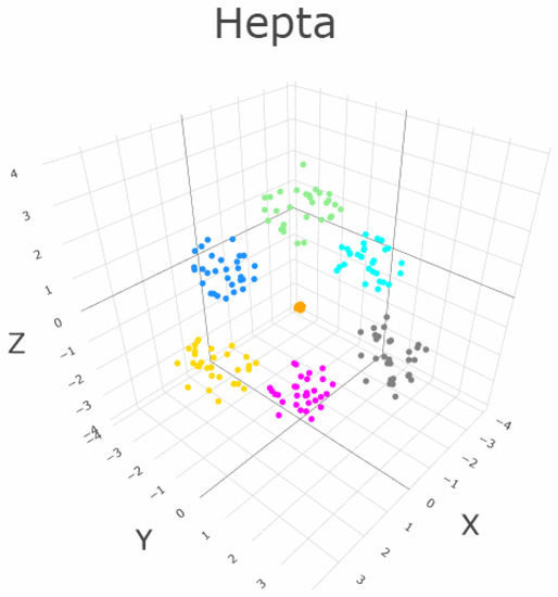
Figure 5.
The three-dimensional Hepta dataset consists of seven clusters that are clearly separated by distance and hyperplanes. One cluster (green) has a higher density [50]. Every cluster is ball-like in shape.
Four dimensionality reduction methods (DR) are chosen: PCA, CCA, Uniform Manifold Approximation Mapping, and t-SNE. For Uniform Manifold Approximation Mapping (IMA) we select parameters appropriately; for t-SNE, we select parameters inappropriately. Figure 6 show the projections once as a scatter plot and once with a visualization of the GCE values per point within the used Gabriel graph. The Uniform Manifold Approximation Mapping projection has low FPE and low BPE.
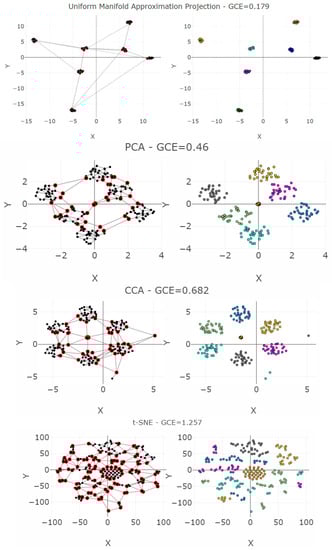
Figure 6.
Projections of four cases of the Hepta dataset into a two-dimensional space. The left-hand plot shows which projected points are connected by edges defined in the Gabriel graph (i.e., are direct neighbors). The GCE considers neighbors of different classes as incorrect (marked in red). The overall GCE value is shown at the top of each plot. (Top first): Uniform Manifold Approximation Projection enables clearly distinguishing the clusters correctly by viewers. (Center): PCA projects the data without disrupting any clusters. This comes close to the best-case scenario for a projection method, although the borders between the clusters are not clearly distinctive. (Bottom second): CCA disrupts two clusters by falsely projecting three points. (Bottom first): When one parameter of the t-SNE algorithm is chosen incorrectly, all clusters are completely disrupted. This is the worst-case scenario for a projection method.
The PCA projection of the Hepta datasets has a low FPE but a higher BPE because although the cluster structures are consistent, the distinction between the clusters is challenging. CCA projection of Hepta generates more than the seven groups that were defined. It has a lower BPE because thestructures are more distinct, but three points have high FPEs. t-SNE projection of Hepta neither preserves neighborhood distances nor the number of clusters. For it, both the FPE and BPE are very high, and the structures cannot be distinguished from each other.
In Figure 7 curves of trustworthiness and continuity (T&D) are drawn for the four projections of the Hepta dataset. The curves tend slightly to prefer the CCA projection over the PCA one. Out of the four cases, the T&D is able to distinguish the worst case of a low structure preservation of t-SNE projection. However, the UMA projection over the PCA/CCA projection preference depends clearly on the range of k. The t-SNE projection disrupts the structures and does not even preserve the distances. Figure 7 shows that the proximities are only preserved for very small values of k. Then the profiles of T&D decrease since larger neighborhoods are not preserved. The T&D profiles for UMA, PCA, and CCA is high at first since close and overall proximities are preserved for neighborhood sizes smaller than the nearly balanced cluster sizes (for Hepta N = 30 for six clusters and N = 36 for the cluster with high density), but decrease after the switching point of knn = 30, because due to the varying density of clusters, not all global distances can be preserved.
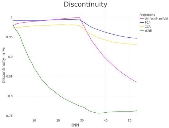
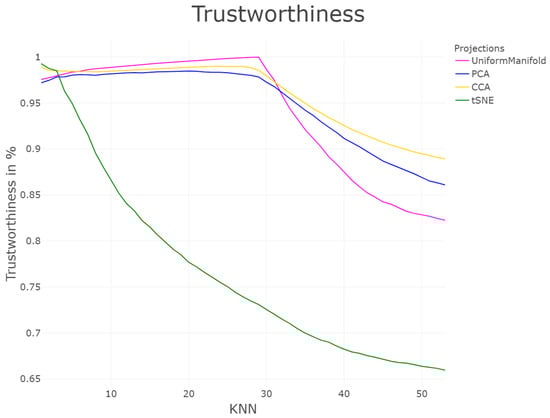
Figure 7.
Profile of structure preservation using trustworthiness and continuity [33] of the four projections for the first 50 k-nearest neighbors. For trustworthiness and discontinuity, the evaluated quality of the projections depends on the interval of k.
In Table 1, the C measures for Cpath and Cwiring (Cp&Cw), Precision and Recal (P&R)l, AUC, Topological Correlation (TC), Topological Index (TI), Zrehen, Classification Error (CE), and the GCE are presented. Lower values for Cp&Cw, P&R, Zrehen, CE, and GCE indicate projections with higher structure preservation. In contrast, higher AUC, TC, and TI values indicate projections with higher structure preservation. It is advisable to inspect Cp with Cw and P with R and select a projection with the lowest values in both QMs. Therefore, if one would weight Cp&Cw or P&R equally, the preference between CCA, PCA, and Uniform Manifold approximation projections remains unclear, although the t-SNE projection yields high values for P&R as well as Cp. The measurement of Zrehen selects the PCA projection as the best with a close second rank to UMA projection. CE has yields for both UMA and PCA projection of zero and this does not distinct them clearly from CCA and t-SNE projections. Calculating AUC in accordance with [26] does not yield proper results because CCA is rated as the best projection by far, while PCA and t-SNE projections yield similar values. In Figure 8, the profile of RAAR starts higher than for the other projections for small k, since the nearest neighbors in the input and output space overlap for k < 4. Then, arrangement of larger neighborhoods from the input space gets disrupted, leading to a strong decrease for higher k. In contrast, the RAAR values for UMAP, PCA, and CCA start small since the nearest neighborhood of the input space is not exactly preserved in the output space, however for growing k starts to overlap stronger since the neighborhood of the input space is preserved on a coarser level. This overlap is maximum when the neighborhood size is the same as the cluster size, which is in Hepta at 30 for almost all clusters. The decrease after the peak is due to the projection errors, which are inevitable for projections of higher dimensions onto lower dimensions. The RAAR (Figure 8) curves do not lead to correct interpretations.

Table 1.
Ten QMs, which produce values of four projections of the Hepta dataset are displayed; Cp = Cpath, Cw = Cwiring, P = Precision, R = Recall, AUC = Area under Curve of RAAR, TC = Topological Correlation, TI = Topological Index, CE = Classification Error, Smoothed Precision and Recall, and GCE = Gabriel Classification Error. The projections are listed in order from best to worst structure preservation. Higher AUC or correlation values denote higher structure preservation. For all other values of QMs, lower values indicate a higher structure preservation of the projection.
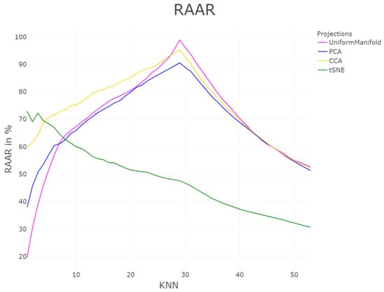
Figure 8.
Profile of structure preservation using Rescaled Average Agreement Rate (RAAR) [26] for knn up to 50. The ranks of best performing DR method depends on the knn. The evaluated quality of the projections depends on the intervall of k.
The five Shepard diagrams have difficulty distinguishing all five cases (Figure A1, see Appendix B). According to the scatter plots, PCA is correlated if density information is disregarded, CCA shows a grouping of distances instead of a linear correlation, similar within the Uniform Manifold Approximation projection and t-SNE, and the distances are randomly distributed. The results of the Shepard diagram contradict Topological index (Table 1), which usually happens if non-linear relationships lie within two variables [51].
In sum, as it is already visible in Figure 6, the GCE per point locally identifies critical points, and the overall sum of the errors clearly distinguishes the four cases.
5.2. Linear Non-Separable Structures of Chainlink
The dataset Chainlink consists of 1000 datapoints in three dimensions [50]. The datapoints are arranged in two separate rings interlocking with each other, which are non-linear separable from one another, see Figure 9. Three DR methods are chosen: t-SNE, PCA, and CCA (see Figure 10). As CCA is stochastic, i.e., its projections depend on the trial, CCA will be applied two times using the same set of parameters. Figure 10 shows the projections, once as a scatter plot and once with a visualization of the measurement points of GCE. The t-SNE projections successfully disentangle the linear non-separable structures of two chains. CCA (1) shows the wrong number of clusters. PCA overlaps the two structures of the original dataset. CCA (2) contains the correct number of clusters. Table 2 shows scalar QMs. Figure 11 and Figure 12 show the RAAR, and trustworthiness and discontinuity profiles.
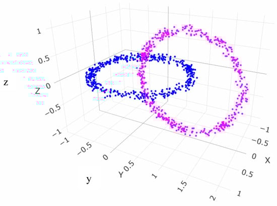
Figure 9.
Two intertwined chains of the Chainlink dataset [50].
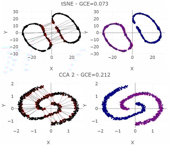
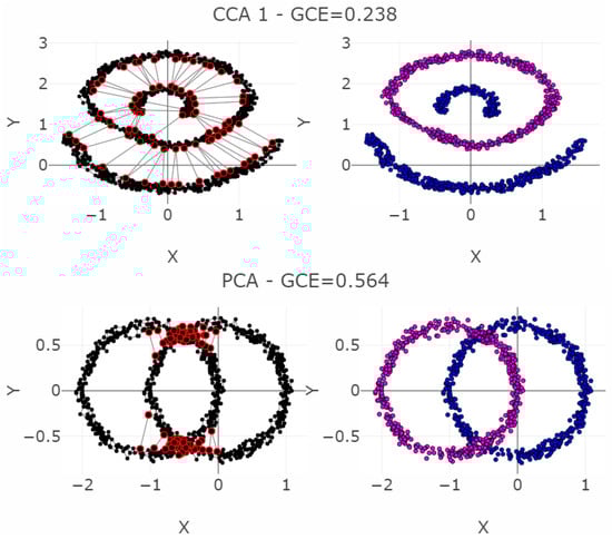
Figure 10.
Projections by the t-SNE, PCA, and CCA methods of the Chainlink data set are presented in the right-hand plots. The colors represent the predefined illness cluster labels. The PCA projection overlaps the clusters, as CCA shows three clearly separated clusters in the first trial (CCA 1) and preserves the cluster structure in the second trial (CCA 2). t-SNE clearly preserves the topology of the rings and separates each structure distinctively from each other. The left-hand plot shows which projected points are connected by edges defined in the Gabriel graph (i.e., are direct neighbors). The GCE considers neighbors of different classes as incorrect (marked in red). The overall GCE value is shown in the top of each plot.
Table 2.
Values of ten QMs for the four projections for the dataset Chainlink. Cp = Cpath, Cw = Cwiring, P = Precision, R = Recall, AUC = Area under Curve of RAAR, TC = Topological Correlation, TI = Topological Index, CE = Classification Error, Smoothed Precision and Recall, and GCE = Gabriel Classification Error. The projections are listed in order from best to worst structure preservation. Higher AUC or correlation values denote higher structure preservation. For all other values of QMs, lower values indicate a higher structure preservation of the projection.
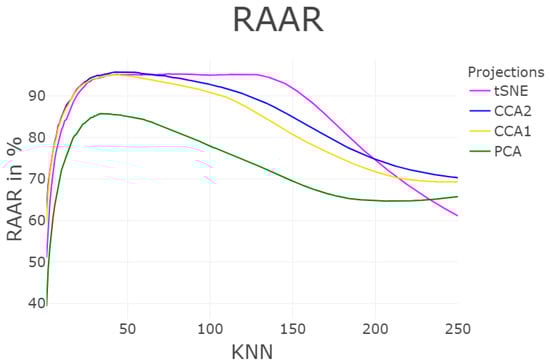
Figure 11.
Profile of structure preservation using Rescaled Average Agreement Rate (RAAR) [26]. The x-axis is in the log scale. CCA performs slightly better than PCA, and the difference between CCA, PCA, and t-SNE to the right of the chart is only visible for knn > 250.
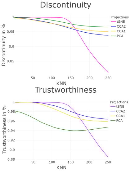
Figure 12.
Profile of structure preservation using T&D for the Chainlink dataset. For discontinuity PCA is clearly regarded as the best projection, while the CCA (2) projection is ideal for trustworthiness up to the first 250 knn, and after that the CCA (1) projection is most suitable. Compared to Figure A2 of the Appendix B, the CCA (1) projection is clearly the best one. Note, that the difference between the three projections is only approximately 3 percent, but the visual differences in Figure A2 are clear.
The PCA projection fails to preserve the structures because PCA maximizes the variance by rotating the input space. However, the structures are linearly non-separable (see Figure 9). The second CCA (2) projection preserves the two structures but the first CCA (1) projection cuts one cluster in half and projects it in the middle of the second cluster, thus disrupting the nonlinearly entangled structures in the input space by letting intruding points in between (see Figure 10). The t-SNE projection clearly separates the two chains in the low-dimensional space. This example illustrates that it is sometimes necessary to make higher BPE/FPE errors for high structure preservation. Here, a trade-off between the structure preservation of the rings and the resulting high FPE in almost all data points can be observed. Hence, the structures can be preserved, but only by introducing higher distances between almost every datapoint by separating the rings in two dimensions further from each other than in the three dimensions. Table 2 presents, then, ten investigated QMs with the same interpretation as in the first example. Besides GCE, none of the measurements clearly distinguish the four cases. Especially CCA which (1 and 2) yield nearly equal values for the QMs.
According to T&D in Figure 12, for k > 1 and k < 40 all projections preserve structures equally well. For k > 40 and k < 155, t-SNE projections has the highest values, thereafter, it is the PCA projection for trustworthiness and CCA (2) projection for discontinuity. CCA (1 and 2) projections are not distinguished clearly. The RAAR in Figure 11 has similar challenges. In total, all three profiles of structure preservation seem to be ambiguous in comparing the quality of the projections with t-SNE with a strong dependence on the parameter while it gives us an either/or situation for the other projections.
The Shepard Density Plot and Topological index are not able to measure which projection preserves the linear non-separable structures appropriately (Figure A2, see Appendix B). This is because the structures of the datasets are not based on global relations between input distances; for every point in one of the rings, there is a point in the other ring such that the given point is closer to it than to its antipodal point. In sum, only GCE values distinguish the apparent cases, as the GCE per point errors are clearly visible in Figure 10.
5.3. High-Dimensional Data of Leukemia
The dataset leukemia consists of a distance matrix covering 554 datapoints [50]. The challenge of leukemia is to recover the high-dimensional structures of the dataset with imbalanced classes. Seven DR methods are applied: MDS, NeRV, CCA, PCA, t-SNE, Sammons Mapping, and emergent self-organizing maps (ESOM), with results presented in Figure 13. Only three DR methods (NeRV, MDS, ESOM) preserve structures without overlap of any classes if the two outliers are disregarded.
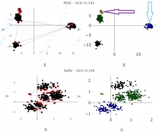
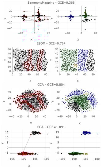
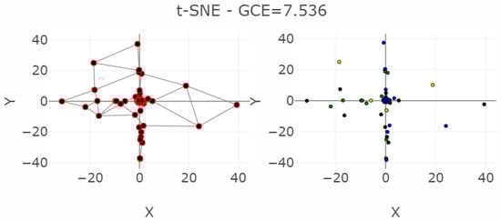
Figure 13.
Projections of the leukemia dataset generated using common methods and the corresponding classification errors for the seven nearest neighbors are presented in the left-hand plots. The colors represent the predefined illness cluster labels. The clusters are separated by empty space in the high-dimensional space. The left-hand plot shows which projected points are connected by edges defined in the Gabriel graph (i.e., are direct neighbors). The GCE considers neighbors of different classes as incorrect (marked in red). The overall GCE value is shown at the top of the plot. The two outliers that lie incorrectly within a group of data in the MDS projection are marked with arrows. The Neighborhood Retrieval Visualizer (NeRV) algorithm splits the smallest class into two roughly equal groups.
For leukemia, the MDS projection distinguishes the four structures in data representing different diagnoses, although one diagnosis (yellow) has a small intra-cluster distance in the output space to another diagnosis (green). Here, two outliers are hidden within the diagnosis of yellow points marked as the magenta point, and the diagnosis consisting of blue points marked as the light blue point. The NeRV projection clearly separates the yellow diagnosis from the other ones. However, the three other diagnoses have small inter-cluster distances to each other, and the green and blue diagnoses are separated in the middle with an intra-cluster distance in the same range as the inter-cluster distances. Therefore, the MDS projection represents the structures visually more clearly than the NeRV projection. This is illustrated in a smaller GCE for the MDS projection in contrast to the NeRV projection. Within the emergent self-organizing map (ESOM) projection [52], the structures in this dataset do not overlap between different classes. However, the separation between the classes is not clearly visible on a mere projection. A third dimension based on the U-heights from the U-matrix [53] can make this separation visible but is disregarded in this analysis. The NeRV projection projects the smallest class into two groups. MDS achieves the best overall structural preservation, though note that two points are mapped into other classes. The light blue outlier data point and the magenta outlier data point are marked with arrows. Their influence on the GCE can be seen from the red nodes in the Gabriel graph of the left-hand plot.
Table 3 presents the values of the QMs with the interpretation explained above, and Figure 14 and Figure 15 visualize the RAAR, and the trustworthiness and discontinuity, respectively. In terms of the smoothed P&R, NeRV projection achieved the best values, and ESOM would be fourth after the projection by Sammons Mapping and MDS. Note the bias in P&R; MDS is clearly distinct in its four different structures in data, although the two outliers lie within the two smaller structures. The overall GCE value here is 0.142, smaller than the GCE of the NeRV projection of 0.194. The precision of the MDS projection is 2194, and the recall is 1074. In contrast, the precision of the NerV projection of the same dataset in Table 3 is 684, and the recall is 1041. Consequently, P&R judges NeRV projection to preserve structures better although the MDS projection depicts the structures better.
Table 3.
Values of ten QMs for the six projections for the dataset leukemia. Cp = Cpath, Cw = Cwiring, P = Precision, R = Recall, AUC = Area under Curve of RAAR, TC = Topological Correlation, TI = Topological Index, CE = Classification Error, Smoothed Precision and Recall, and GCE = Gabriel Classification Error. The projections are listed in order from best to worst structure preservation. Higher AUC or correlation values denote higher structure preservation. For all other values of QMs, lower values indicate a higher structure preservation of the projection. The TC could not be computed for leukemia due to the proportion of dimensions and number of points in the data set.
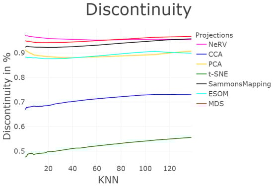
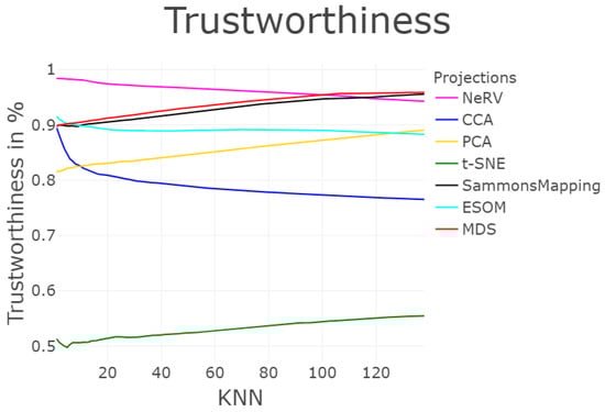
Figure 14.
Profile of structure preservation using T&D measurements for the six projections shown in Figure 13 of the leukemia dataset. The discontinuity is highest for Sammon Mapping and NeRV (top left), as is the trustworthiness (top right). However, in the case of trustworthiness, the outcome depends on the number of nearest neighbors considered, k; for a low value, ESOM is superior to Sammon Mapping, and for a high value, principal component analysis (PCA) overtakes NeRV. Without the scatter plots in Figure A3, interpretation of the results of this Figure is difficult.
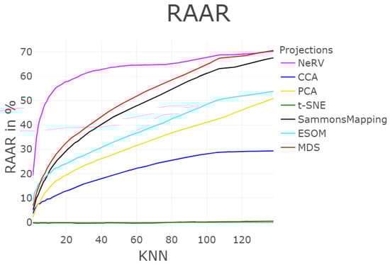
Figure 15.
Profile of structure preservation using Rescaled Average Agreement Rate (RAAR) [26]. The ranks of the projection vary depending on the knn, which is computed for up to 138 neighbors.
Based on the Cp and CW values, the user would either select NeRV projection or CCA or MDS depending on the user’s decision to either judge Cp or Cw as more important, with the PCA projection being a close second. In AUC, the NeRV is considered as the best; for TI, it is MDS. For Zrehen, it is either MDS, Sammons Mapping, or PCA projection, for the CE values MDS, NeRV, and ESOM projection yield highly similar values with NerV and MDS being slightly better.
The discontinuity profile in Figure 14, depending on the range of k either NeRV or MDS would be selected as the best choice. In terms of the profile of trustworthiness for k < 100 NeRV would be the best choice, otherwise Sammons Mapping and MDS perform better. For the profile of RAAR (Figure 15) profiles clearly depicts NeRV as the best projection. In contrast to Figure 7 and Figure 8, in Figure 14 and Figure 15, no switching point is apparent in the functional profiles. Our hypothesis is that the reason for this may be due to the unbalanced cluster sizes.
6. Discussion
This work aims to propose a quality measurement (QM) that focuses on structure preservation. Structure preservation in this case refers to the preservation of groups of data points that are homogeneous, i.e., distinctable by either distance or density. Especially, the aim is to penalize points intruding into regions of the output space belonging to other separable structures of the input space. Thus, structure preservation should be measured in terms of the separation of higher-dimensional structures in their lower-dimensional representation. Consequently, FPE is allowed if the close neighbors in the input space, mapped far from each other on the output space, are still accounted in the same structure. These errors are not always avoidable, depending on the geometry or topology of the classes. For example, imagine a sphere hull with a dense core in three dimensions projected onto two dimensions. The properties of the hull cannot be preserved in two dimensions, however, the assignment to the structure of dense core versus hull can be preserved. By similar reasoning, BPE is allowed to some degree as well. In order to preserve separable structures, the focus lies on gaps, i.e., it is more important to avoid points of clearly separate classes from being projected close to each other than it is to attempt to arrange the points perfectly according to some global objective, e.g., preserving the global distances of the input space . Hence, a QM is required to account for those circumstances in order to measure the structure preservation of projections. Such a QM should have the following properties:
- The result should be easily interpretable and should enable a comparison of different DR methods.
- The result should be deterministic, with no or only simple parameters.
- The result should be statistically stable and calculable for high-dimensional data in .
- The result should measure the preservation of high-dimensional linear and nonlinear structural separability.
In this work, 19 QMs were reviewed. Given the definition of structure preservation, it is possible to group QMs into semantic classes based on graph theory. Overall, there are three major semantic classes: compact, connected, and non-generalizable. Since the non-generalizable QMs are restricted in their applicability regarding the underlying type of DR method, they are discarded for lack of generality. The other two semantic classes are based on a general concept of neighborhood defined through graph theory. The connected-based QMs are divided into two sub-classes: unidirectional and direction-based. Based on the classification of the QMs into semantic groups, here, one is able to identify several approaches that have not yet been considered. For example, one could develop a QM based on unit disk graphs. Theoretical analysis shows that the 19 QMs, based on their semantic classes, depend on prior assumptions regarding the underlying high-dimensional structures of interest (for further QM definitions, see Appendix A).
Based on the theoretical analysis performed in this work, structure preservation is about preserving neighbourhoods with a specific extent. Several approaches that we defined within the class of compact measurements tried to measure the preservation of all distances, which seems not advisable if DR methods are used to project high-dimensional data into the two-dimensional space. Alternatives are summarized in the class named connected, which distinguishes at least between direction-based and unidirectional neighborhoods (See Figure 2) of various extents. For unidirectional neighborhoods, various approaches like MCMC (see Appendix A), RAAR, or T&D propose the solve the challenge to an appropriate extent by measuring a functional profile. Except for GCE, a similar approach of direction-based techniques was not proposed yet.
Classical DR methods were applied, such as t-distributed stochastic neighbor embedding [54], which is a nonlinear focusing dimensionality reduction method, PCA [55], a linear dimensionality reduction method that maximizes the variance of the given data, CCA [56], a focusing dimensionality reduction method which preserves local distances prior to global distances, NeRV [8], a focusing non-linear dimensionality reduction method which optimizes the trade-off between precision and recall, emergent self-organizing map (ESOM) [52], which is a self-organizing map with thousands or ten thousands of neurons and Uniform Manifold Approximation projection. Projections were generated on three datasets.
The presented artificial datasets are generated to contain a specific structure concept for which specific sample sizes can be generated [50]. A detailed description and further examples can be found in [50], although some are two-dimensional and hence, not usable to evaluate DR methods. The FCPS datasets are accessible in [57]. Furthermore, the three datasets used in this work have a predefined ground truth, which is mandatory for an unbiased benchmarking study. Hepta is selected as it poses the challenge of non-overlapping convex hulls with varying intra-cluster distances [50]. Chainlink is selected as it poses the challenge of linear non-separable entanglements [50]. Leukemia is a high-dimensional (d > 7000) dataset with highly imbalanced cluster sizes from 2.7% to 50% [49]. The leukemia dataset is selected because the classification (i.e., diagnoses) is reflected by the previously investigated structures in the data [48].
The artificial dataset ‘Hepta’ (Figure 5) [50] provides well-defined linear separable structures and the artificial dataset ‘Chainlink’ (Figure 9) [50] provides well-defined linear non-separable structures. The natural dataset leukemia consists of more than d = 7000 dimensions but they are clearly separable [47,49]. For each semantic class we evaluated a selection of often-used representative QMs on projections of the above methods of artificial and real-world high-dimensional datasets with different DR methods designed for projection on two dimensions. The QMs reviewed here seemingly do not capture the relevant errors that occur in the projections of the DR method because they assume certain definitions regarding the types of neighborhoods that should be preserved (see also Appendix A). As a consequence, the presented QMs are biased as they assume specific structure in data, and sometimes use specific projection methods, e.g., Shepard diagram and stress for MDS and Sammons Mapping.
QMs for evaluating the preservation of compact structures like the Shepard diagram are easily interpretable because they measure the quality of the preservation of all distances or dissimilarities. In most cases, the outcome is a single value in a specified range. However, no projection is able to completely preserve all distances or even the ranks of the distances [58,59,60]. Hence, we argue that only the preservation of dissimilarities or distances between separate structures is important but not within similarities. Therefore, any attempt to measure the quality of a projection by considering all distances is greatly disadvantageous. For example, the major disadvantage of the stress and the C measure is that the largest dissimilarity, which is likely associated with outliers in the data, exerts the strongest influence on the F value. Moreover, the C measures do not consider gaps. In our experiment with the dataset containing linear non-separable structures, called Chainlink, the linear correlation measurements did not yield the correct rankings and favored the linear projection PCA. Similarly, outliers resulting in extreme distances are over-weighted in all correlation approaches, and the preservation of essential neighborhoods reduces the correlation values.
Connected QMs compare only local neighborhoods H. For unidirectional connected QMs, choosing the correct number of k-nearest neighbors is necessary, which is a complicated problem. If the range is selected inappropriately, the connected QMs are not able to precisely rank the best projections. This is mainly because the profiles of RAAR and T&D yield varying results for different numbers of the nearest-neighbor k. It is unclear which range of k to prefer and how to interpret a result in which the trustworthiness profile for a projection is high but the discontinuity profile is low.
Even worse, for comparing different projection methods, it may be necessary to choose different knn values for the output space if there is a need to measure structure preservation. For this reason, unidirectional QMs that result in a single value, such as König’s measure [61], do not satisfy quality conditions I and II. In other approaches, e.g., MRRE and T&D, two F values are obtained for every knn, and it is necessary to plot both functions, as profiles. In this case, no distinction is possible between gaps and FPEs. Any further comparison of functional profiles for different DR methods is abstract and, consequently, not easily interpretable. Notably, the co-ranking matrix framework defined in [28,62] allows for the comparison, from a theoretical perspective, of several QMs (the MRRE, T&D, and LCMC) based on ). However, no transformation of the co-ranking matrix into a single meaningful value exists [6], and the practical application of co-ranking matrices is controversial [63]. With regard to the LCMC, ref. [64] showed that it is statistically unstable and not smooth. Consequently, conditions I and II are not met, but the KNN graph is always calculable (IV).
Cw & Cp, as well as P&R, have to be interpreted together; therefore, it remains up to the user to define a weight between them. An optimal recall or Cw indicates low FPE, whereas an optimal precision or Cp indicates low BPE. Our results show that they do not allow distinct structure preservation appropriately. However, in this example, the recall of the PCA projection is judged to be more structure-preserving than Sammons Mapping and comes very close to NeRV. Moreover, P&R considers the NeRV projection to preserve structures compared to the MDS projection as higher, although the MDS projection clearly depicts the structures in a better way. Thus, P&R does not reflect the problem of overlapping structures. Instead, it automatically favors NeRV that internally optimizes P&R. As a consequence, NeRV projections will always receive a high rating in P&R. Additionally, a choice based on the P&R quality is difficult, it is challenging since CCA (2) projection achieves a successful projection, yet is ranked closer to the worse projections than to the other successful projection t-SNE. Hence, a new QM is required to measure the quality of structure preservation independent of a definition of an objective function, assuming a prior classification is accessible in order to put weight on certain FPEs and BPEs above others conditionally.
Investigated direction-based QMs also encounter difficulties in evaluating structure preservation, although they have the advantage that a distinction between FPEs and gaps is possible. However, an obvious disadvantage is the very high cost of calculation: for a Delaunay graph with rising dimensionality d. [65]. Villmann et al. [66] attempted to solve this problem by proposing an approximation of the intrinsic dimension of [67]. In theory, the TF (see Appendix A for definition) seems to be the best choice, but in the context considered here, a projection is defined as a mapping into a lower-dimensional space. In this case, the QM F(h) is equal to zero for h < 0. It follows that F(h = 0) = F(h = 1) + F(h = −1) = F(h = 1). Consequently, half of the definition proves to be useless for the purpose considered here. The second problem is that the TF does not consider the input distances apart from calculating the Delaunay graph in the input space. Thus, there is no difference between FPE and BPE as long as no other points lie in between. Further disadvantages include numerical instability because the Delaunay graph is sensitive to rounding errors in higher dimensions and the fact that the Delaunay graph does not always correctly preserve neighborhoods if the intrinsic dimensionality of the data does not match the dimensionality of the output space O [41]. The results of this work show that the QM of Zrehen does not reflect the BPE in almost every case.
Furthermore, the problem of trial-dependent projections is demonstrated in the example of the CCA projection of the Chainlink dataset. Choosing the best method out of a trial based on one of the ten investigated QM does not necessarily yield the best structure preservation.
Therefore, we can conclude that QMs are biased with the bias depending on their semantic class. They will favor the algorithm which is closest to the definition of the QM without considering the structures within the data. For example, Precision and Recall will always favor NeRV projections.
In sum, each QM has challenges in evaluating the projection. Either the ranks are wrong, the differences in the projections are not reflected, or the correct number of neighbors to evaluate a neighbor-dependent QM is not clear.
As a consequence, a new QM is proposed in this work, namely the Gabriel Classification Error (GCE). The GCE is independent of the objective function used by a projection method and avoids a bias towards particular structures within the data. The GCE focuses on preserving local neighborhoods in the sense that structures of the input data should be clearly separable in the projection, though a lesser focus is set on the distance preservation interior to a structure. Separate structures in the data are defined by separate labels in either a given prior classification or a clustering of data. FPE and BPE are only measured when relevant regarding structures from other classes. In cases, where two structures from different classes are close or touching in that sense of the empty ball condition, an error is accounted for. In addition, the GCE allows projections to be ranked and compared with a baseline in a normalized manner in the range of [−2, 2].
As seen from the previous section, the GCE demonstrated the expected behavior for model data (Hepta and Chainlink) and ranked the projections preserving the separability of data appropriately. The Uniform Manifold Approximation projection of Hepta generates the most negligible errors. Similar to Chainlink, the CCA (2) recovering each structure at its whole suffers from fewer errors than the CCA (1), which splits the structure in two, for which the difference is quite low, reflecting the potential to recover structures and the separability, followed by the PCA with high errors accounted for the overlap of the two ring structures. Lastly, we can use the same explanations of GCE for Leukemia: the NeRV projection achieves the second-best GCE after the MDS projection, which shows a clear separation of the structures, followed by Sammons Mapping and ESOM, respectively. The presented artificial datasets are generated to contain a specific structure concept for which specific sample sizes can be generated [50]. A detailed description and further examples can be found in [50]. The FCPS datasets are accessible in [57], although some are two-dimensional and hence, not usable to evaluate DR methods.
GCE only penalizes those datapoints which have a neighborhood connection with datapoints from another class in the Gabriel graph sense. The penalty is weighted according to the distance rank of the neighbor in the sense of the input space. The distances within a neighborhood of data points of the same class are not penalized (see Figure 6, Figure 10 and Figure 13—left vs. right). Due to this penalization approach, GCE requires a classification vector. This limits the usage of the GCE to datasets for the classification is either identified by cluster analysis or defined through prior knowledge (c.f. [49] for discussion). Furthermore, the GCE weighs errors higher with an increasing number of connections to data points from other classes. Thus, cutting structures of one class increases the GCE the same as BPE and FPE between different classes. However, the BPE and FPE within one class are not measured. Similar to the classification error, the GCE requires a classification vector. Comparable to Zrehens measures, GCE uses the Gabriel graph in the output space but GCE only measures errors if different classes are involved in weighting each with a harmonic weight and their high-dimensional distances in the input space. In contrast, Zrehens accounts only for data points, which are closer to the point of interest in the input space but not inside the empty ball, thus, all points that violate the empty ball condition. Similar to the profiles of T&D and RAAR, resulting errors are weighted based on the k-nearest neighbors, but in the case of GCE, the weight is determined with a harmonic function and only if at least one of the neighboring points in the Gabriel graph is of a different class than the point of interest, otherwise not accounting an error at all. However, the GCE could not be reproduced by any weighting of the other QMs, since the canceling out of errors depends on the classification vector, which is not available for the presented QMs except for the CE.
Based on the work of de Berg et al. [68], it follows that the expected time complexity of generating the Gabriel graph of a set of planar points is The generation Delaunay graph has an expected complexity [69]. Then, one can iterate over its ) edges and check for every vertex if it violates the open ball condition for this very edge with an expected space complexity of (c.f. theorem 9.12 of [68]). It should be noted that there are claims of algorithms of lower complexity [70,71].
The advantage of GCE is the simple interpretation and a sensitive differentiation between different cases. The major limitation is that the GCE obviously requires a classification vector forcing prior knowledge about the task yet still allows the benchmarking of dimensionality reduction methods.
Moreover, GCE can support the successful interaction of a Human-in-the-Loop [72], providing a classification vector with DR methods to investigate the relationships between data and classification [73]. Additionally, the GCE visualization enables the user to examine the projection’s quality and could, in the future, be implemented interactively. Such interactivity would break down the mathematical complexity of choosing parameters or a DR method or finding trade-offs between DR methods. For example, GCE could potentially add another metric to visualization tools like SubVIS, an interactive visualization tool to explore subspace clusters from different perspectives [74]. When choosing subspaces for subspace clustering, the ones preserving separability might be favorable. Hence, the GCE could be incorporated into the subspace choice function of such an approach [74].
In future work, it is essential to systematically benchmark dimensionality reduction methods based on priorly defined structures to provide a guideline for data scientists. Here, GCE allows projections to be ranked and compared to a baseline in the range of [−2, 2]. Although the theoretical analysis and the examples used to indicate that the GCE is a valid alternative in estimating the quality of projections, an additional human evaluation study could be advisable. Such a study will investigate if human experts prefer the GCE over other quality measurements.
7. Conclusions
We have discovered the bias in each of the presented quality measurements (QM) for dimensionality reduction (DR) methods. These QMs fall into two semantic classes, namely compact and connected based on the underlying graph used. Compact QMs evaluated all the dissimilarities of the high-dimensional data set. The connected type is based on the neighborhood concept. We demonstrate that QMs fail to measure the quality of projection if the structures in the data do not meet the bias of the QM. Therefore, we propose a new QM, the Gabriel Classification Error (GCE), which focuses on the preservation of classifications in the neighborhoods of data points; in particular, knowledge about the structure must be given in the form of a classification prior to the computation. The goal is to measure the quality of the projection, defined as structure preservation unbiased towards the input data and method. The GCE is available as an R package on CRAN https://CRAN.R-project.org/package=DRqualityt (accessed on 11 July 2023).
Author Contributions
Conceptualization, M.C.T.; methodology, M.C.T.; software, M.C.T., J.M. and Q.S.; validation, J.M. and Q.S.; formal analysis, J.M., M.C.T. and Q.S.; investigation, M.C.T.; resources, M.C.T.; data curation, M.C.T.; writing—original draft preparation, M.C.T., J.M. and Q.S.; writing—review and editing, J.M. and Q.S.; visualization, Q.S.; supervision, M.C.T.; project administration, M.C.T. All authors have read and agreed to the published version of the manuscript.
Funding
This research received no external funding.
Data Availability Statement
Data is available in [50].
Conflicts of Interest
The author Quirin Stier is employed by IAP-GmbH Intelligent Analytics Project. The owner of the company is Michael Thrun. The collaboration of Thrun and Stier was mainly conducted in the context of a research relationship between the respective authors at the University of Marburg where Michael Thrun is a senior lecturer (in ger.: “Privatdozent”) and Quirin Stier is one of his doctoral candidates. The author Julian Märte has been involved as a consultant in IAP-GmbH Intelligent Analytics Project in several projects. Note, however, the consultation of Märte for IAP-GmbH did not have any influence on the outline, data acquisition, analysis, or discussion of the results presented in this research work.
Appendix A
Appendix A.1. More Quality Measures and Preservation of High-Dimensional Distances in the Two-Dimensional Space
Appendix A.1.1. Force Approach Error
According to the force approach concept presented in [75], the relation between the distances and should be constant for each pair of adjacent data points. The force approach attempts to separate data points that are projected too close to one another and to bring together those that are too scattered. In [75], it was suggested that it is possible to improve any projection method by the following means:
First, for each pair of projected points , the vector is calculated if is a direct neighbor of ; then, a perturbation in the direction of is applied. Consequently, is moved in the direction of by the fraction defined in (A1). When all points have thus been improved, a new iteration begins.
Note that all distances are normalized only once. For performance reasons, the projected points are normalized in every iteration instead of the . The error on the projected points is defined as:
Thus, as shown in Equation (A1), the force approach error is defined with respect to a Euclidean graph, and an F value of zero suggests optimal neighborhood preservation, as seen from Equation (A2). A similar approach, referred to as point compression and point stretching, was proposed in [18], where it was used for the visualization of errors with the aid of Voronoi cells.
Appendix A.1.2. König’s Measure
König’s measure is a rank-based measure introduced in [76]:
with , as in Equation (A4)
König’s measure is controlled by the following parameters: a constant parameter c and a variable parameter representing the neighborhood size, , which must be smaller than c.
In the first case, the ranks place l in the same knn neighborhood with respect to j in both the input and output spaces. In the second case, the sequence in the neighborhood may be different, but is still within the first knn ranks relative to j in the current neighborhood defined by the value of knn. In the third case, the point l lies in a larger, constant neighborhood of .
The range of F is between zero and one, where a value of one indicates perfect structure preservation and a value of zero indicates poor structure preservation [61]. The parameters and c were investigated by [37]. The results indicated that c does not have a strong influence on the value of F; F changes only for large knn values. Moreover, [37] showed that the parameter influences only the magnitude of the F value, whereas the form of F(knn) remains approximately the same.
Appendix A.1.3. Local Continuity Meta-Criterion (LCMC)
The local continuity meta-criterion (LCMC) was introduced in [77]; note that a similar idea was independently adopted by [78]. Because the correlation between these two measures is very high [9], only the LCMC is introduced here. The LCMC is defined as the average size of the overlap between neighborhoods consisting of the k-nearest neighbors in I and O [64]. For each and , there exist corresponding sets of points in the neighborhoods and , which are calculated using a given knn in a KNN graph. The overlap is measured in a pointwise manner:
In Equation (A5), a global measure is obtained by averaging all N cases [64]. The mean is normalized with respect to knn because this value is the upper bound on . Equation (A6) is also adjusted by means of a baseline term representing a random neighborhood overlap, which is obtained by modeling a hypergeometric distribution with knn defectives out of N − 1 items, from which knn items are drawn:
In contrast to the T&D measures and the mean relative rank error (MRRE; see the next section), the LCMC is calculated based on desired behavior [28]. The cited authors also showed that the LCMC can be expressed as a special case of the co-ranking matrix.
Appendix A.1.4. Mean Relative Rank Error (MRRE) and the Co-Ranking Matrix
The MRRE was introduced in [79] and is defined as follows:
The normalization is given by , which represents the worst case. There are notable similarities between the MRRE and the T&D measures: both types of measures use the ranks of the distances and KNN graphs to calculate overlaps, but, in addition to the different weightings, the MRRE also measures changes in the order of positions in a neighborhood H(knn, I) or H(knn, O). Both position changes and intruding/extruding points are considered, but position changes are weighted more heavily than intrusion/extrusion. The MRRE (and T&D and LCMC, as well) can be abstracted using the co-ranking matrix framework as follows:
As introduced in [27], is a matrix in which each element is equal to the number of pairs of points that lie in neighborhoods defined by the same or different values of knn. For example, represents the upper left block of the co-ranking matrix for a specific knn. Formally, Q is a sum of N permutation matrices; hence, . It was shown in [28] that the MRRE can be rewritten as two alternative quantities characterizing a projection:
, which the authors call the quality of the projection, and , called the behavior (for details, see [28]).
Appendix A.1.5. Topographic Product
The topographic product [80] and an improved version thereof [81] were originally defined for neural maps, but in contrast to the quantization error [42] and the topographic error [43], it is possible to generalize the idea of the topographic product to all projection methods. Let the points constitute the neighborhood of a point j in a metric space M defined based on a knn graph and sorted in ascending order of knn; then,
Q represents the distance between the point j and the k-th nearest neighbor in the input space I divided by the distance between the point j and the point corresponding to the k-th nearest neighbor in O. Now, the product of q and Q of Equations (A9) and (A10) for all orders knn can be calculated in Equation (A11):
The resulting QM is then defined as:
F takes different values depending on whether the dimension of the output space is smaller than (F < 0), similar to (F 0), or greater than (F > 0) the dimension of the input space [81]. Thus, in our case, F is always smaller than zero. Revuelta et al. [81] improved the topographic product by using the shortest-path distances in a Euclidean graph (geodesic distances) in Equations (A13) and (A14) instead of the direct distances of Equations (A9) and (A10):
Appendix A.1.6. Topographic Function (TF)
The topographic function (TF) for SOMs was introduced in [82]. This measure operates on Voronoi tessellations [12]. The TF quantifies the identity of the Delaunay graphs in I and O [83]. This work follows the general definitions found in [66], where the TF is defined as given in Equation (A15) (denoted by F), with being the cardinality of 0 or :
The shortest path in the Delaunay graph of the input space between the data points ) is denoted by , and that between the projected points ) is denoted by . The Delaunay–graph distances G and g are equal to the number of Voronoi cells between the two points. If h is greater than zero, then ) are neighbors in the input space, and if h is smaller than zero, then ) are neighbors in the output space.
In Equation (A16), represents the number of neighbors surrounding a data point at a Delaunay distance greater than h, with the restriction that only the projected points that are located in adjacent Voronoi cells in O are considered.
The converse situation is considered in Equation (A17): represents the number of neighbors surrounding a projected point at a Delaunay distance greater than h, with the restriction that only the data points that are located in adjacent Voronoi cells in I are considered.
In summary, the shape of enables a detailed discussion of the magnitude of distortions occurring in O [41]: “Small values of h indicate that there are only local dimensional conflicts, whereas large values indicate the global character of a dimensional conflict” [66]. Bauer et al. [41] proposed the following simplified equation:
Here, h is equal to zero if and only if two points are neighbors in both the input space and the output space; thus, the overlap of Voronoi neighbors in I and O is required.
Appendix A.1.7. U-Ranking
In [17], a QM based on a lattice was proposed. To generalize the idea to any projection method, one would use a graph. Let be a graph, and let g(l, j,) be the shortest path between the projected points ; then, the U-distance can be generalized as:
Let be the ascending sequence of all U-distances, as defined in Equation (A19), with respect to an arbitrary projected point j. The rank represents the position in the consecutive sequence of all U-distances with respect to a projected point . Now, the minimal U-ranking measure can be defined as follows:
Considering [84], a good choice for is the Delaunay graph .
Appendix B. Shepard Diagrams Visualized as Density Plot
The Shepard diagrams are generated with the R package “DataVisualizations” available on CRAN (https://CRAN.R-project.org/package=DataVisualizations, accessed on 11 July 2023) [51]. A two-dimensional density estimation and coloring procedure is used [85] available as an R package on CRAN (https://CRAN.R-project.org/package=ScatterDensity, accessed on 11 July 2023). The color scale changes with increasing density from blue to green, yellow, orange and red [85]. Two-dimensional density approach is used to estimate the density of the points in each scatter plot [85].
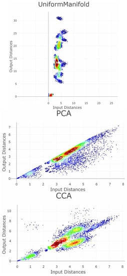
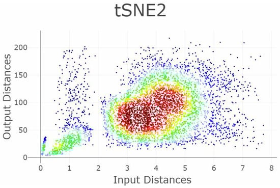
Figure A1.
Density scatter plots of the Shepard diagrams [29] of the five projections of the Hepta dataset shown in Figure 6. Using a two-dimensional density estimation approach, the colors of the points are defined. The colorscale changes with increasing density from blue to green, yellow, orange and red [85]. Based on the Shepard diagrams, PCA and CCA best preserve the distances in the data.
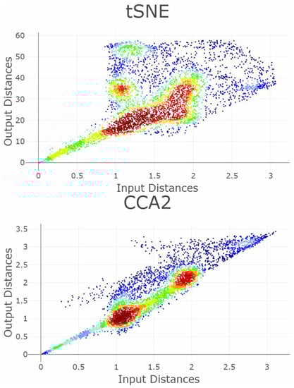
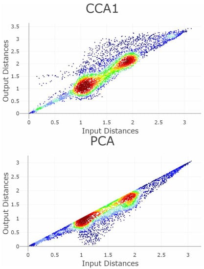
Figure A2.
Density scatter plots of the Shepard diagrams (density plots) for four projections of the Chainlink dataset. Using a two-dimensional density estimation approach, the colors of the points are defined. The colorscale changes with increasing density from blue to green, yellow, orange and red [85]. PCA appears to preserve the distances best, but in reality, it results in the worst structure preservation (see the Appendix A). No clear difference between the CCA projections can be distinguished. The best projection from t-SNE shows strong correlation with some disturbance, which could be ranked last based only on the Shepard density diagrams presented here.
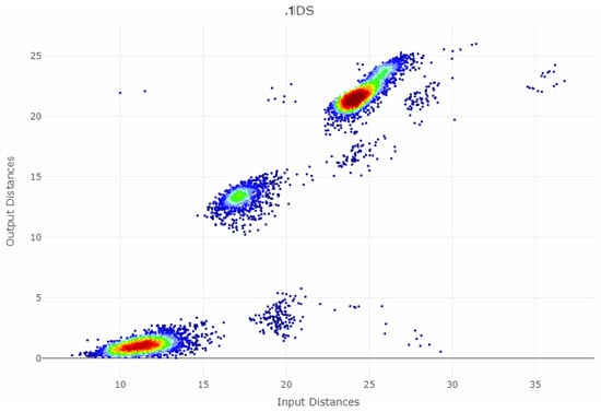
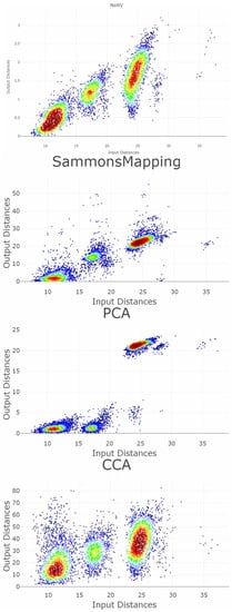
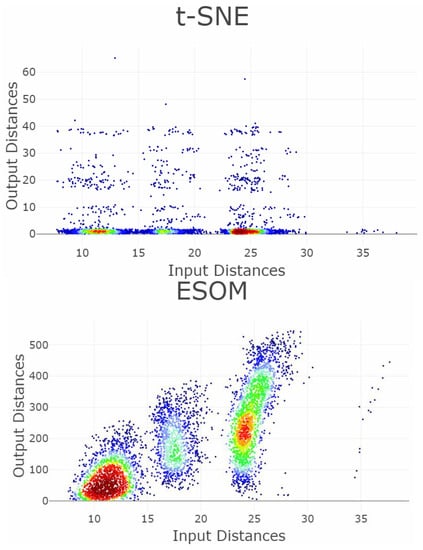
Figure A3.
Density scatter plots of the Shepard diagrams for six projections of the leukemia dataset. Using a two-dimensional density estimation approach, the colors of the points are defined. The colorscale changes with increasing density from blue to green, yellow, orange and red [85]. In each plot, multiple distinct aggregations of input vs. output distances of varying size, density, and form are visible.
Appendix C
Appendix C.1. Parameter Settings and Source Code Availability
The parameter settings for the clustering algorithms, the projection methods and the QMs used in this work are as follows:
Appendix C.1.1. Quality Measures (QMs)
Freely available implementations of the trustworthiness and discontinuity (T&D) measures and the precision and recall (P&R) measures in C++ code were used (see R package ProjectionBasesClustering on CRAN). For all other measures, self-developed implementations were used available in the R package “DRquality” on CRAN (https://CRAN.R-project.org/package=DRquality, accessed on 11 July 2023).
Appendix C.1.2. Projection Methods
For the projection methods considered here we used freely available code which is summarized in the ProjectionBasedClustering CRAN package. For principal component analysis (PCA) [86], we used the PCA software available in the R package stats [87]; for curvilinear component analysis (CCA) [56], the CCA source code was ported from MATLAB to R and for t-distributed stochastic neighbor embedding (t-SNE), we used Donaldson’s t-SNE implementation. Also included in the evaluation of various projection methods were the Neighbor Retrieval Visualizer (NeRV) algorithm [8] as implemented in the freely available C++ code called in R., the Sammon Mapping technique for multidimensional scaling (MDS) [88] available from [87], and the emergent self-organizing map (ESOM) algorithm as implemented in the R package Umatrix available on CRAN (https://CRAN.R-project.org/package=Umatrix, accessed on 11 July 2023).
For every projection method, only the default parameters were used, as given here. The ESOM algorithm was set with 20 epochs; a planar lattice; 50 lines; 80 columns; a Euclidean neighborhood function; and a linear annealing scheme with a starting radius of 25, an end radius of 1, a starting learning rate of 0.5, and an end learning rate of 0.1.
For the NeRV method, lambda was set to 0.1 (default); the optimization scheme was set with 20 neighbors, 10 iterations, 2 conjugate gradient steps per iteration, and 20 conjugate gradient steps in the final iteration, and the points were randomly initialized (default). PCA and Sammon Mapping did not require any input parameters. For CCA, 20 epochs, an initial step size of 0.5, and a radius of influence of 3∗ were specified. The t-SNE method was set with a perplexity of 30, 100 epochs, and a maximum number of iterations of 1.000. Every projection method is available through standardized wrappers in our R package projections on CRAN. The NeRV source code was modified only as required for compatibility with the CRAN package Rcpp.
References
- Everitt, B.S.; Landau, S.; Leese, M. Cluster Analysis; Arnold: London, UK, 2001. [Google Scholar]
- Mirkin, B.G. Clustering: A Data Recovery Approach; Chapman & Hall/CRC: Boca Raton, FL, USA, 2005. [Google Scholar]
- Ritter, G. Robust Cluster Analysis and Variable Selection; Chapman & Hall/CRC Press: Passau, Germany, 2014. [Google Scholar]
- Hennig, C.; Meila, M. Handbook of Cluster Analysis; Chapman & Hall/CRC Press: Boca Raton, FL, USA, 2015. [Google Scholar]
- van der Maaten, L.J.; Postma, E.O.; van den Herik, H.J. Dimensionality reduction: A comparative review. J. Mach. Learn. Res. 2009, 10, 66–71. [Google Scholar]
- Mokbel, B.; Lueks, W.; Gisbrecht, A.; Hammer, B. Visualizing the quality of dimensionality reduction. Neurocomputing 2013, 112, 109–123. [Google Scholar] [CrossRef]
- Yin, H. Nonlinear dimensionality reduction and data visualization: A review. Int. J. Autom. Comput. 2007, 4, 294–303. [Google Scholar] [CrossRef]
- Venna, J.; Peltonen, J.; Nybo, K.; Aidos, H.; Kaski, S. Information retrieval perspective to nonlinear dimensionality reduction for data visualization. J. Mach. Learn. Res. 2010, 11, 451–490. [Google Scholar]
- Gracia, A.; González, S.; Robles, V.; Menasalvas, E. A methodology to compare Dimensionality Reduction algorithms in terms of loss of quality. Inf. Sci. 2014, 270, 1–27. [Google Scholar] [CrossRef]
- Ray, P.; Reddy, S.S.; Banerjee, T. Various dimension reduction techniques for high dimensional data analysis: A review. Artif. Intell. Rev. 2021, 54, 3473–3515. [Google Scholar] [CrossRef]
- Ayesha, S.; Hanif, M.K.; Talib, R. Overview and comparative study of dimensionality reduction techniques for high dimensional data. Inf. Fusion 2020, 59, 44–58. [Google Scholar] [CrossRef]
- Toussaint, G.T. The relative neighbourhood graph of a finite planar set. Pattern Recognit. 1980, 12, 261–268. [Google Scholar] [CrossRef]
- Delaunay, B. Sur la sphere vide. 1934. Available online: http://galiulin.narod.ru/delaunay_.pdf (accessed on 11 July 2023).
- Gabriel, K.R.; Sokal, R.R. A new statistical approach to geographic variation analysis. Syst. Biol. 1969, 18, 259–278. [Google Scholar] [CrossRef]
- Brito, M.; Chávez, E.; Quiroz, A.; Yukich, J. Connectivity of the mutual k-nearest-neighbor graph in clustering and outlier detection. Stat. Probab. Lett. 1997, 35, 33–42. [Google Scholar] [CrossRef]
- Clark, B.N.; Colbourn, C.J.; Johnson, D.S. Unit disk graphs. Discret. Math. 1990, 86, 165–177. [Google Scholar] [CrossRef]
- Ultsch, A.; Herrmann, L. The architecture of emergent self-organizing maps to reduce projection errors. In Proceedings of the 13th European Symposium on Artificial Neural Networks (ESANN), Bruges, Belgium, 27–29 April 2005; pp. 1–6. [Google Scholar]
- Aupetit, M. Visualizing distortions and recovering topology in continuous projection techniques. Neurocomputing 2007, 70, 1304–1330. [Google Scholar] [CrossRef]
- Mair, F.; Hartmann, F.J.; Mrdjen, D.; Tosevski, V.; Krieg, C.; Becher, B. The end of gating? An introduction to automated analysis of high dimensional cytometry data. Eur. J. Immunol. 2016, 46, 34–43. [Google Scholar] [CrossRef] [PubMed]
- Ultsch, A.; Lötsch, J. Machine-learned cluster identification in high-dimensional data. J. Biomed. Inform. 2017, 66, 95–104. [Google Scholar] [CrossRef] [PubMed]
- Bunte, K.; Biehl, M.; Hammer, B. A general framework for dimensionality-reducing data visualization mapping. Neural Comput. 2012, 24, 771–804. [Google Scholar] [CrossRef]
- Goodhill, G.J.; Finch, S.; Sejnowski, T.J. Quantifying Neighbourhood Preservation in Topographic Mappings; Chapman & Hall/CRC: Boca Raton, FL, USA, 1995. [Google Scholar]
- Durbin, R.; Mitchison, G. A dimension reduction framework for understanding cortical maps. Nature 1990, 343, 644–647. [Google Scholar] [CrossRef] [PubMed]
- Mitchison, G. A type of duality between self-organizing maps and minimal wiring. Neural Comput. 1995, 7, 25–35. [Google Scholar] [CrossRef]
- Hinton, G.E.; Roweis, S.T. Stochastic neighbor embedding. In Advances in Neural Information Processing Systems; MIT Press: Cambridge, MSA, USA, 2002; pp. 833–840. [Google Scholar]
- Lee, J.A.; Peluffo-Ordonez, D.H.; Verleysen, M. Multiscale stochastic neighbor embedding: Towards parameter-free dimensionality reduction. In Proceedings of the 22nd European Symposium on Artificial Neural Networks, Computational Intelligence And Machine Learning (ESANN), Bruges, Belgium, 23–25 April 2014. [Google Scholar]
- Lee, J.A.; Verleysen, M. Rank-based quality assessment of nonlinear dimensionality reduction. In Proceedings of the 16th European Symposium on Artificial Neural Networks (ESANN), Bruges, Belgium, 23–15 April 2008; pp. 49–54. [Google Scholar]
- Lee, J.A.; Verleysen, M. Quality assessment of dimensionality reduction: Rank-based criteria. Neurocomputing 2009, 72, 1431–1443. [Google Scholar] [CrossRef]
- Shepard, R.N. Multidimensional scaling, tree-fitting, and clustering. Science 1980, 210, 390–398. [Google Scholar] [CrossRef]
- Kruskal, J.B. Multidimensional scaling by optimizing goodness of fit to a nonmetric hypothesis. Psychometrika 1964, 29, 1–27. [Google Scholar] [CrossRef]
- Kruskal, J.B. Nonmetric multidimensional scaling: A numerical method. Psychometrika 1964, 29, 115–129. [Google Scholar] [CrossRef]
- Venna, J.; Kaski, S. Neighborhood preservation in nonlinear projection methods: An experimental study. In Artificial Neural Networks—ICANN 2001; Springer: Berlin/Heidelberg, Germany, 2001; pp. 485–491. [Google Scholar]
- Kaski, S.; Nikkilä, J.; Oja, M.; Venna, J.; Törönen, P.; Castrén, E. Trustworthiness and metrics in visualizing similarity of gene expression. BMC Bioinform. 2003, 4, 48. [Google Scholar] [CrossRef] [PubMed]
- Siegel, S.; Castellan, N.J. Nonparametric Statistics for the Behavioural Sciences; McGraw-Hill: New York, NY, USA, 1988. [Google Scholar]
- Bezdek, J.C.; Pal, N.R. An index of topological preservation and its application to self-organizing feature maps. In Proceedings of the 1993 International Conference on Neural Networks (IJCNN-93-Nagoya, Japan), Nagoya, Japan, 25–29 October 1993; pp. 2435–2440. [Google Scholar]
- Bezdek, J.C.; Pal, N.R. An index of topological preservation for feature extraction. Pattern Recognit. 1995, 28, 381–391. [Google Scholar] [CrossRef]
- Karbauskaitė, R.; Dzemyda, G. Topology preservation measures in the visualization of manifold-type multidimensional data. Informatica 2009, 20, 235–254. [Google Scholar] [CrossRef]
- Handl, J.; Knowles, J.; Dorigo, M. Ant-based clustering and topographic mapping. Artif. Life 2006, 12, 35–62. [Google Scholar] [CrossRef] [PubMed]
- Doherty, K.; Adams, R.; Davey, N. Topological correlation. In Proceedings of the 14th European Symposium on Artificial Neural Networks (ESANN), Bruges, Belgium, 26–28 April 2006; pp. 125–130. [Google Scholar]
- Zrehen, S. Analyzing Kohonen maps with geometry. In ICANN’93; Springer: Berlin/Heidelberg, Germany, 1993; pp. 609–612. [Google Scholar]
- Bauer, H.-U.; Herrmann, M.; Villmann, T. Neural maps and topographic vector quantization. Neural Netw. 1999, 12, 659–676. [Google Scholar] [CrossRef]
- Uriarte, E.A.; Martín, F.D. Topology preservation in SOM. Int. J. Math. Comput. Sci. 2005, 1, 19–22. [Google Scholar]
- Kiviluoto, K. Topology preservation in self-organizing maps. In Proceedings of the International Conference on Neural Networks, Washington, DC, USA, 3–6 June 1996; pp. 294–299. [Google Scholar] [CrossRef]
- Cunningham, J.P.; Ghahramani, Z. Linear dimensionality reduction: Survey, insights, and generalizations. J. Mach. Learn. Res. 2015, 16, 2859–2900. [Google Scholar]
- Pölzlbauer, G. Survey and comparison of quality measures for self-organizing maps. In Proceedings of the Fifth Workshop on Data Analysis (WDA′04), Vysoké Tatry, Slovakia, 13–15 June 2003; pp. 67–82. [Google Scholar]
- Beaton, D.; Valova, I.; MacLean, D. CQoCO: A measure for comparative quality of coverage and organization for self-organizing maps. Neurocomputing 2010, 73, 2147–2159. [Google Scholar] [CrossRef]
- Thrun, M.C.; Ultsch, A. Swarm Intelligence for Self-Organized Clustering. Artif. Intell. 2021, 290, 103237. [Google Scholar] [CrossRef]
- Thrun, M.C.; Pape, F.; Ultsch, A. Conventional Displays of Structures in Data Compared with Interactive Projection-Based Clustering (IPBC). Int. J. Data Sci. Anal. 2021, 12, 249–271. [Google Scholar] [CrossRef]
- Thrun, M.C. Distance-Based Clustering Challenges for Unbiased Benchmarking Studies. Nat. Sci. Rep. 2021, 11, 18988. [Google Scholar] [CrossRef] [PubMed]
- Thrun, M.C.; Ultsch, A. Clustering Benchmark Datasets Exploiting the Fundamental Clustering Problems. Data Brief 2020, 30, 105501. [Google Scholar] [CrossRef] [PubMed]
- Thrun, M.C.; Ultsch, A. Effects of the payout system of income taxes to municipalities in Germany. In Proceedings of the 12th Professor Aleksander Zelias International Conference on Modelling and Forecasting of Socio-Economic Phenomena, Cracow, Poland, 8–11 May 2018; pp. 533–542. [Google Scholar]
- Ultsch, A. Data mining and knowledge discovery with emergent self-organizing feature maps for multivariate time series. In Kohonen Maps, 1st ed.; Oja, E., Kaski, S., Eds.; Elsevier: Amsterdam, The Netherlands, 1999; pp. 33–46. [Google Scholar]
- Ultsch, A.; Mörchen, F. ESOM-Maps: Tools for Clustering, Visualization, and Classification with EMERGENT SOM; University of Marburg: Marburg, Germany, 2005. [Google Scholar]
- Van der Maaten, L.; Hinton, G. Visualizing Data using t-SNE. J. Mach. Learn. Res. 2008, 9, 2579–2605. [Google Scholar]
- Hotelling, H. Analysis of a complex of statistical variables into principal components. J. Educ. Psychol. 1933, 24, 417. [Google Scholar] [CrossRef]
- Demartines, P.; Hérault, J. CCA: “Curvilinear component analysis”. In Proceedings of the 15° Colloque sur le Traitement du Signal et des Images, Antibes, France, 18–21 September 1995. [Google Scholar]
- Thrun, M.C.; Stier, Q. Fundamental Clustering Algorithms Suite. SoftwareX 2021, 13, 100642. [Google Scholar] [CrossRef]
- Drygas, H. Über multidimensionale Skalierung. Stat. Pap. 1978, 19, 63–66. [Google Scholar] [CrossRef]
- Kirsch, A. Bemerkung zu H. Drygas, “Über multidimensionale Skalierung”. Stat. Pap. 1978, 19, 211–212. [Google Scholar] [CrossRef]
- Schmid, F. Über ein Problem der mehrdimensionalen Skalierung. Stat. Pap. 1980, 21, 140–144. [Google Scholar] [CrossRef]
- König, A. Interactive visualization and analysis of hierarchical neural projections for data mining. IEEE Trans. Neural Netw. 2000, 11, 615–624. [Google Scholar] [CrossRef]
- Lee, J.A.; Verleysen, M. Scale-independent quality criteria for dimensionality reduction. Pattern Recognit. Lett. 2010, 31, 2248–2257. [Google Scholar] [CrossRef]
- Lueks, W.; Mokbel, B.; Biehl, M.; Hammer, B. How to Evaluate Dimensionality Reduction?-Improving the Co-ranking Matrix. arXiv 2011, arXiv:1110.3917. [Google Scholar]
- Chen, L.; Buja, A. Local multidimensional scaling for nonlinear dimension reduction, graph drawing, and proximity analysis. J. Am. Stat. Assoc. 2009, 104, 209–219. [Google Scholar] [CrossRef]
- Aupetit, M. Robust Topology Representing Networks. In Proceedings of the 11th European Symposium on Artificial Neural Networks (ESANN), Bruges, Belgium, 23–25 April 2003; pp. 45–50. [Google Scholar]
- Villmann, T.; Der, R.; Herrmann, M.; Martinetz, T.M. Topology preservation in self-organizing feature maps: Exact definition and measurement. IEEE Trans. Neural Netw. 1997, 8, 256–266. [Google Scholar] [CrossRef] [PubMed]
- Grassberger, P.; Procaccia, I. Estimation of the Kolmogorov entropy from a chaotic signal. Phys. Rev. A 1983, 28, 2591–2593. [Google Scholar] [CrossRef]
- De Berg, M.; van Kreveld, M.; Overmars, M.; Schwarzkopf, O. Computational Geometry: Algorithms and Applications; Springer: New York, NY, USA, 2008. [Google Scholar]
- Shamos, M.I.; Hoey, D. Closest-point problems. In Proceedings of the 16th Annual Symposium on Foundations of Computer Science (sfcs 1975), Berkeley, CA, USA, 13–15 October 1975; pp. 151–162. [Google Scholar]
- Bhattacharya, B.; Mukherjee, K.; Toussaint, G. Geometric decision rules for high dimensions. In Proceedings of the 55th Session of the International Statistics Institute, Sydney, Australia, 5–12 April 2005. [Google Scholar]
- Matula, D.W.; Sokal, R.R. Properties of Gabriel graphs relevant to geographic variation research and the clustering of points in the plane. Geogr. Anal. 1980, 12, 205–222. [Google Scholar] [CrossRef]
- Holzinger, A. Interactive machine learning for health informatics: When do we need the human-in-the-loop? Brain Inform. 2016, 3, 119–131. [Google Scholar] [CrossRef]
- van Unen, V.; Höllt, T.; Pezzotti, N.; Li, N.; Reinders, M.J.; Eisemann, E.; Koning, F.; Vilanova, A.; Lelieveldt, B.P. Visual analysis of mass cytometry data by hierarchical stochastic neighbour embedding reveals rare cell types. Nat. Commun. 2017, 8, 1740. [Google Scholar] [CrossRef]
- Hund, M.; Böhm, D.; Sturm, W.; Sedlmair, M.; Schreck, T.; Ullrich, T.; Keim, D.A.; Majnaric, L.; Holzinger, A. Visual analytics for concept exploration in subspaces of patient groups. Brain Inform. 2016, 3, 233–247. [Google Scholar] [CrossRef]
- Tejada, E.; Minghim, R.; Nonato, L.G. On improved projection techniques to support visual exploration of multi-dimensional data sets. Inf. Vis. 2003, 2, 218–231. [Google Scholar] [CrossRef]
- König, A.; Bulmahn, O.; Glesner, M. Systematic Methods for Multivariate Data Visualization and Numerical Assessment of Class Separability and Overlap in Automated Visual Industrial Quality Control. In Proceedings of the British Machine Vision Conference, BMVC 1994, York, UK, 31 August–3 September 1994; pp. 19.1–19.10. [Google Scholar]
- Chen, L.; Buja, A. Local Multidimensional Scaling for Nonlinear Dimensionality Reduction, Graph Layout, and Proximity Analysis; University of Pennsylviana: Philadelphia, PA, USA, 2006. [Google Scholar]
- Akkucuk, U.; Carroll, J.D. PARAMAP vs. Isomap: A comparison of two nonlinear mapping algorithms. J. Classif. 2006, 23, 221–254. [Google Scholar] [CrossRef]
- Lee, J.A.; Verleysen, M. Nonlinear Dimensionality Reduction; Springer: New York, NY, USA, 2007. [Google Scholar]
- Bauer, H.-U.; Pawelzik, K.R. Quantifying the neighborhood preservation of self-organizing feature maps. IEEE Trans. Neural Netw. 1992, 3, 570–579. [Google Scholar] [CrossRef]
- Revuelta, F.F.; Chamizo, J.M.G.; Rodríguez, J.G.; Sáez, A.H. Geodesic topographic product: An improvement to measure topology preservation of self-organizing neural networks. In Advances in Artificial Intelligence–IBERAMIA 2004; Springer: Berlin/Heidelberg, Germany, 2004; pp. 841–850. [Google Scholar]
- Villmann, T.; Der, R.; Herrmann, M.; Martinetz, T.M. A novel approach to measure the topology preservation of feature maps. In ICANN’94; Springer: Berlin/Heidelberg, Germany, 1994; pp. 298–301. [Google Scholar]
- Herrmann, L. Swarm-Organized Topographic Mapping. Doctoral Dissertation, Philipps-Universität Marburg, Marburg, Germany, 2011. [Google Scholar]
- Lötsch, J.; Ultsch, A. Exploiting the Structures of the U-Matrix. In Proceedings of the Advances in Self-Organizing Maps and Learning Vector Quantization, Mittweida, Germany, 2–4 July 2014; Villmann, T., Schleif, F.-M., Kaden, M., Lange, M., Eds.; Springer International Publishing: Berlin/Heidelberg, Germany, 2014; pp. 249–257. [Google Scholar]
- Brinkmann, L.; Stier, Q.; Thrun, M.C. Computing Sensitive Color Transitions for the Identification of Two-Dimensional Structures. In Proceedings of the Data Science, Statistics & Visualisation (DSSV) and the European Conference on Data Analysis (ECDA), Antwerp, Belgium, 5–7 July 2023; p. 57. [Google Scholar]
- Pearson, K. LIII. On lines and planes of closest fit to systems of points in space. Lond. Edinb. Dublin Philos. Mag. J. Sci. 1901, 2, 559–572. [Google Scholar] [CrossRef]
- R Development Core Team. R: A Language and Environment for Statistical Computing, 3.2.5; R Foundation for Statistical Computing: Vienna, Austria, 2008. [Google Scholar]
- Sammon, J.W. A nonlinear mapping for data structure analysis. IEEE Trans. Comput. 1969, 18, 401–409. [Google Scholar] [CrossRef]
Disclaimer/Publisher’s Note: The statements, opinions and data contained in all publications are solely those of the individual author(s) and contributor(s) and not of MDPI and/or the editor(s). MDPI and/or the editor(s) disclaim responsibility for any injury to people or property resulting from any ideas, methods, instructions or products referred to in the content. |
© 2023 by the authors. Licensee MDPI, Basel, Switzerland. This article is an open access article distributed under the terms and conditions of the Creative Commons Attribution (CC BY) license (https://creativecommons.org/licenses/by/4.0/).