Mssgan: Enforcing Multiple Generators to Learn Multiple Subspaces to Avoid the Mode Collapse

Abstract

Generative Adversarial Networks are powerful generative models that are used in different areas and with multiple applications. However, this type of model has a training problem called mode collapse. This problem causes the generator to not learn the complete distribution of the data with which it is trained. To force the network to learn the entire data distribution, MSSGAN is introduced. This model has multiple generators and distributes the training data in multiple subspaces, where each generator is enforced to learn only one of the groups with the help of a classifier. We demonstrate that our model performs better on the FID and Sample Distribution metrics compared to previous models to avoid mode collapse. Experimental results show how each of the generators learns different information and, in turn, generates satisfactory quality samples.

1. Introduction

Generative Adversarial Networks [1] (GANs) are generative models of artificial intelligence that learn a data distribution and generate a sample from it. These models have grown rapidly by demonstrating their potential by generating realistic samples from the distribution of the data on which they were trained.

The architecture of GANs has two agents competing with each other. A generative model learns to map data from domain z to domain x and generates realistic samples to try to fool the other agent. On the other hand, a discriminator model has the task of distinguishing whether the sample comes from the data distribution or was generated by the generative model.

These networks have proven to be a powerful tool in different tasks, such as generating images through text [2], superresolution of images [3], video synthesis [4], rendering realistic photorealistic images from the virtual world [5], translation from a source domain to a different target domain [6], generating natural protein sequence diversity [7], and a mix of multiple medical applications such as reconstruction, segmentation, and generation of images, classification, and detection of diseases [8].

Several works have focused on enhancing the quality of images generated with GAN architectures. For instance, state-of-the-art models like StyleGAN [9] and its improvements, StyleGAN2 [10] and StyleGAN3 [11], propose a novel generator architecture in GAN models that is based on styles, enabling an automatic and unsupervised separation of high-level attributes. The generator starts with a learned constant input and adjusts the style of the image at each convolutional layer based on the latent space, allowing direct control over image features at different scales. Additionally, these models combine this architecture with injected noise directly into the network, enabling stochastic variation in the generated images. Through the evaluation of generated images using the Frechet Inception Distance (FID) metric, the superiority in terms of image quality compared to other GAN architectures is demonstrated. However, it is worth noting that models like these have an enormous number of trainable parameters, with this particular model boasting 26.2 million parameters, making training infeasible on many computer systems due to its high computational cost.

However, despite the great capabilities demonstrated by these models, GANs have problems during training. One of the most common problems is mode collapse, as it does not allow the generator to fully learn the distribution of the training data [12].

The mode collapse can be divided into partial and total collapse. The partial mode collapse occurs when the generative agent leads to mapping only a part of the data of training and misses a great part of the real distribution. The total mode collapse is when the generator produces samples that fool the discriminator, but these samples are not similar to the training data.

Mode collapse can occur when the generator finds a small number of samples that fool the discriminator. The generator would be inclined to find a single mode that always fools the discriminator and would start to map every sample to this space. If this occurs, the gradient of the loss function collapses near 0. When mode collapse is presented during training, the generator can become numb to its input and therefore has no incentive to diversify its output. Even if we retrain the discriminator, the generator can find another mode that fools the discriminator [13].

Different variants have been proposed to tackle mode collapse. Wasserstein GAN (WGAN) [14] adopts the Wasserstein distance in the loss function to measure the dissimilarity between the real data distribution and the generated data distribution, but this model needs to satisfy 1-Lipshitz continuity and this causes the gradients to disappear or explode under various scenarios. To solve the problem of WGAN, a Gradient Penalty is added in WGAN-GP [15] to enforce the 1-Lipschitz and avoid the vanishing gradient. Another proposal, called Boundary Equilibrium Generative Adversarial Network (BEGAN) [16], changes the discriminator for an AutoEncoder (AE) and balances the loss function between the generator and the discriminator. This model learns the latent space of the image while balancing the generator and discriminator. However, BEGAN also suffers from mode collapse from not being able to fully learn a useful and structured latent space. In the BEGANv3 proposal [17], they used a Variational AutoEncoder (VAE) that added statistical techniques to the AE to try to avoid mode collapse in GANs.

The strategy of adding multiple generators to address mode collapse is motivated by the limitations of a single generator to learn different modes. The Mixture Generators Adversarial Network (MGAN) [18] employs a mixture of generators with shared parameters to train all generators simultaneously. Since there are no restrictions requiring generators to learn all modes, these generators tend to learn the same modes, resulting in producing identical samples. To try to ensure that each generator learns different data, Multi-Generator Orthogonal GAN (MGO-GAN) [19] employs a strategy to construct orthogonal vectors based on the output of the generators, and enforces that the generators contain different information during training. However, the multiple generators of the MGO-GAN model can learn similar or very identical data distributions; this causes the outputs of the generators to be redundant. The model can still lose some modes from the real distribution since the architecture is based on learning different data distribution, but can not force the generators to learn all real data distribution. Under certain parameters, one mode can be learned for several generators of MGO-GAN if these generators learn different information from the same mode.

Using multiple generators within a clustering framework, such as MSSGAN, offers advantages across various scenarios. First, it proves beneficial when working with intricate datasets featuring diverse modes or categories, allowing for the comprehensive capture of data distributions. For example, in image generation, generators can specialize in specific categories, like cats and dogs, yielding more diverse and precise results. Second, by training each generator to focus on specific data subsets, it enhances the quality and variety of generated samples within each category, a critical factor in applications like image synthesis. Lastly, in situations involving imbalanced datasets with underrepresented classes or modes, employing multiple generators can rectify the imbalance during generation, ensuring that minority classes receive adequate attention during training and resulting in more balanced content in terms of class representation.

With changes in either the loss function or in the architecture of the models, the mode collapse still appears during training in different GANs. This is why we propose an approach called Multi Sub Space GAN (MSSGAN) to train multiple generators each with a different mode and tackle the mode collapse problem. In our approach, the training data (total space) is separated into multiple clusters (subspaces), with the number of clusters equal to the number of generators to train. All data in each cluster are labeled according to the cluster to which they belong. A classifier is trained with these data and labels. The generators are forced to learn only a part of the original data distribution, with the help of the subspace and the classifier. Each generator learns to generate data from one cluster passing its output through a pre-trained classifier. The output of the pre-trained classifier is added to the loss function of the generator. This strategy forces the generators to learn different information and at the same time to learn different modes of the real distribution.

In this study, we make the following contributions:

• To the best of our knowledge, MSSGAN is the first work based on multiple generators that learn independent regions of the data space to overcome the mode collapse.
• MSSGAN strategy is easily applicable to previous GANs.
• MSSGAN achieves a better performance obtaining the same or even better scores in metrics to evaluate the mode collapse compared to models used as baseline.

2. Materials and Methods

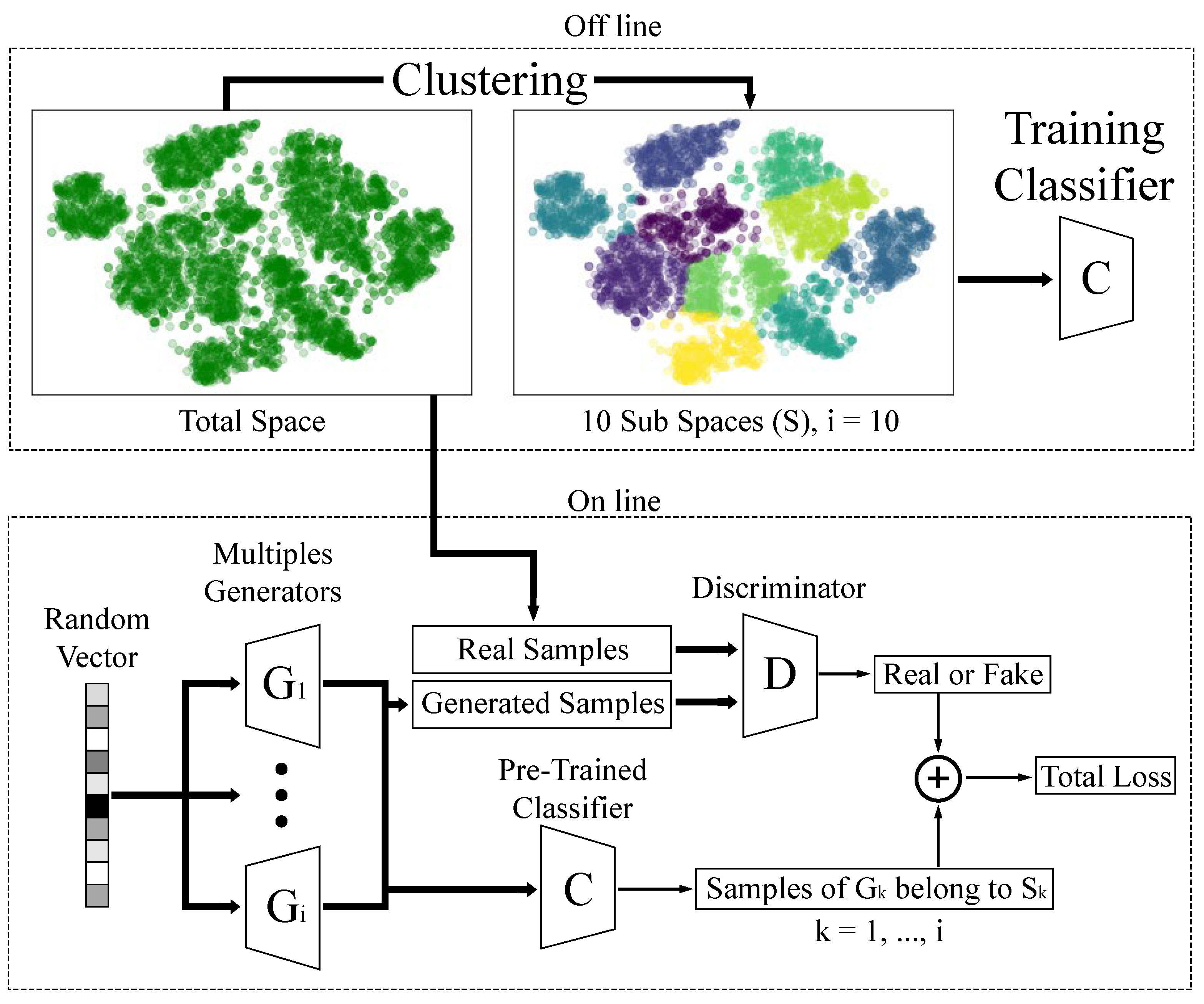
The overall methodology is shown in Figure 1, which consists of two steps: (a) an offline step, where the data are clustered into groups equal to the number of generators that the model will be trained. These groups are called subspaces. With this subspaces a classifier is trained to identify which group the input sample belongs to. (b) After the offline step, the generators are trained and the classifier is used to enforce the output of each generator.

To train the model, a random vector of size 100 is the input of each generator, and the generator tries to produce samples identical to the real samples. These outputs of the generator are used to train the discriminator where its job is to identify whether the samples come from one of the generators or from the real data. The outputs of each generator are passed through the pre-trained classifier. The work of the classifier is to enforce each generator to produce identical samples from only one group, where the generator $G_k$ produces identical samples from the subspace $S_k$, where $(k=1,\dots ,i)$ and i is the total number of subspaces.

2.1. MSSGAN Architecture

The MSSGAN model is based on an architecture consisting of three main agents: the discriminator, the generators, and the classifier. Unlike traditional GAN models, the MSSGAN model employs a multi-generative architecture, which means it utilizes a set of generators $G_{1:k}$, where k is the number of generators in the model, based on the number of subspaces the training database was divided into.

Each generator in the model is responsible for generating samples from a particular subspace of the database. These samples are combined to produce a complete sample, which is then fed to the discriminator for evaluation. The discriminator assesses whether the sample is real or fake, i.e., whether it comes from the training dataset or was generated by the model.

A classifier is trained to distinguish to which subspace each input sample belongs. The classifier is trained in the pre-training phase using a labeled dataset, where each sample is labeled with the corresponding subspace it belongs to. Once trained, the classifier is used in the second phase of training to guide the sample generation of the model.

2.2. Pre-Training

The pre-training phase in the MSSGAN model consists of two important tasks. The first task involves creating subspaces in which the training database will be divided. The second task is training the classifier using the labeled dataset, where the labels indicate the subspace to which each sample belongs.

For the first task, let us assume we have a dataset S, which we will consider as the overall space. To create subspaces, we need to divide the dataset into smaller and distinct subsets. These subsets will be called subspaces. The idea behind this division is that subspaces can contain similar features, which will help the classifier make more accurate predictions. Additionally, it helps the generators achieve better results by generating data with similar characteristics, as they have a simpler task of generating data with similar features in each subspace.

For a training database, the set S would consist of all the data samples that will be used to train the model. To divide the training data into subspaces, a clustering algorithm is employed. This algorithm groups samples that are similar to each other into the same subspace. Then, a label is assigned to each sample, indicating which subspace it belongs to.

After labeling all the samples, the second task during the pre-training phase is to train a classifier to learn how to distinguish which subspace each input data belongs to. The classifier uses the subspace labels as class labels and is trained using supervised learning techniques. In this way, the classifier can assign a subspace label to each new sample that is presented in the future, enabling the MSSGAN model to work with multiple generators and subspaces during training.

Each subspace created using the clustering algorithm is associated with a distinct generator in the MSSGAN model. This means that each generator is responsible for creating samples only for its specific subspace, with the assistance of the classifier that identifies the subspace to which each sample belongs.

This association between subspaces and generators allows each generator to focus solely on generating samples for its assigned subspace, instead of having to generate samples for all the subspaces. Moreover, by forcing each generator to work in its own subspace, it promotes specialization among the generators and improves the quality of the generated samples.

2.3. Loss Function Objective

2.3.1. GAN Objective

The standard GAN has two agents, a generator and a discriminator. The generator learns to map samples to the distribution $p_g$ over the data x, with an input z to represent a space $G\left(z\right)$, where G is the output of the generator. On the other hand, the discriminator D evaluates the probability that the data come from the training data distribution $p_x$ or from $p_g$. The Discriminator and Generator play a minmax game with the loss function of the model (1), this loss function is based on the Jensen-Shannon divergence (JSD):

$$mi{n}_{G}ma{x}_{D}V(G,D)=logD\left(x\right)+log(1-D(G\left(z\right)\left)\right)$$

(1)

D is trained to maximize (1), the loss function of the discriminator is (2), while G is trained to minimize it, and the loss function of the generator is (3) .

$$\begin{array}{c}\hfill {\mathcal{L}}_D=logD\left(x\right)+log(1-D\left(G\left(z\right)\right))forD\end{array}$$

(2)

$$\begin{array}{c}\hfill {\mathcal{L}}_G=log(1-D\left(G\left(z\right)\right))forG\end{array}$$

(3)

2.3.2. Wasserstein Distance

WGAN introduced the Wasserstein Distance in GANs. This distance is based on the Earth Move Distance (EMD), which is the metric that measures the minimum effort to transform one data distribution into another. The function (4) shows the loss function when GAN is training with this distance. Equation (5) shows the loss function for D while G is shown in (6).

$$mi{n}_{G}ma{x}_{D}V(G,D)=D\left(x\right)-D\left(G\left(z\right)\right)$$

(4)

$$\begin{array}{c}\hfill {\mathcal{L}}_D=D\left(x\right)-D\left(G\left(z\right)\right)forD\end{array}$$

(5)

$$\begin{array}{c}\hfill {\mathcal{L}}_G=-D\left(G\left(z\right)\right)forG\end{array}$$

(6)

2.3.3. Classifier Objective

The classifier is an agent that learns to predict the class to which a given input z belongs. To work, the classifier has the following cross-entropy loss function:

$${\mathcal{L}}_C=-\sum _{j=1}^C{t}_{j}log\left(p_j\right)$$

(7)

where $t_j$ is the target label, $p_j$ is the softmax probability of the jth class and C the number of classes. The output of the classifier $C\left(z\right)$, given an input z, is the probability that z belongs to each of the classes with which the classifier was trained.

2.3.4. MSSGAN Loss Function

MSSGAN strategy is easily modifiable, this model can employ different loss functions like JSD and Wasserstein Distance. Likewise, the architecture can be trained with a different number of generators.

We employ a set of generators $G_{1:k}$ where k is the number of generators and, therefore, the number of subspaces into which the training set is clustered. The loss function of standard GAN or Wasserstein GAN is defined for only one generator; in this way, the loss functions (1) and (4) are transformed to apply multiple generators. The MSSGAN model adds a loss function that is given by the classifier. The samples generated by each generator are passed as pre-trained classifier input to obtain the labels of which group these samples belong to. This is to enforce the generator to produce samples from a single cluster. With this method, the output samples of each generator must belong to only one of the cluster.

When the model works with loss function JSD, the function (1) is modified to apply to multiple generators and add the error of not generating samples of the corresponding subspace, and this last error is given by the classifier. With this loss function and the modifications, we obtain the following function:

$$mi{n}_{G_{1:k},C_{1:k}}ma{x}_{D}V(G_{1:k},C_{1:k},D)=logD\left(x\right)+\frac{1}{k}\sum _{i=1}^k\left[log(1-D\left(G_i\left(z\right)\right))+\beta \ast C\left(G_i\left(z\right)\right)\right]$$

(8)

Thus, the loss functions of the discriminator (9) and generators (10) are

$${\mathcal{L}}_D=logD\left(x\right)+\frac{1}{k}\sum _{i=1}^k\left[log(1-D\left(G_i\left(z\right)\right))\right.\left.+\beta \ast C\left(G_i\left(z\right)\right)\right]forD$$

(9)

$${\mathcal{L}}_G=log(1-D\left(G\left(z\right)\right))+\beta \ast C\left(G\left(z\right)\right)foreachG$$

(10)

On the other hand, the transform of loss function Wasserstein Distance (4) to apply for MSSGAN is presented below:

$$mi{n}_{G_{1:k},C_{1:k}}ma{x}_{D}V(G_{1:k},C_{1:k},D)=D\left(x\right)-\frac{1}{k}\sum _{i=1}^k\left[D\left(x\right)+\beta \ast C\left(G_i\left(z\right)\right)\right]$$

(11)

The loss function of the discriminator (12) and generators (13) are

$${\mathcal{L}}_D=D\left(x\right)-\frac{1}{k}\sum _{i=1}^k\left[D\left(G_i\left(z\right)\right)\right.\left.+\beta \ast C\left(G_i\left(z\right)\right)\right]forD$$

(12)

$${\mathcal{L}}_G=-D\left(G\left(z\right)\right)+\beta \ast C\left(G\left(z\right)\right)foreachG$$

(13)

where $\beta$ is used to give more or less weight to the correct label of the samples generated by the generators in its corresponding group. Algorithm 1 shows the algorithm for training the MSSGAN model, where initial ${\mathcal{L}}_{D_G}=0$.

Algorithm 1 Training of MSSGAN.

for number of epoch do     for i = number of generators do         Create a batch N from $G_i$         Calculate ${\mathcal{L}}_{D_G}={\mathcal{L}}_{D_G}-\frac{1}{N}{\sum }_{n=1}^N\left[D\left(x^n\right)\right]$     end for     Create a batch M from real distribution     Caluclate ${\mathcal{L}}_D=\frac{{\mathcal{L}}_{D_G}}{i}+\frac{1}{M}{\sum }_{m=1}^N\left[D\left(x^m\right)\right]$     Update Discriminator     for i = number of generators do         Create a batch N from $G_i$         Calculate ${\mathcal{L}}_G=-\frac{1}{N}{\sum }_{n=1}^N\left[D\left(x^n\right)\right]+\frac{\beta }{N}{\sum }_{n=1}^N\left[C\left(x^n\right)\right]$         Update Generator i     end for end for

2.4. Metrics of Evaluation Mode Collapse

To evaluate the mode collapse and the correct distribution between the distinct modes, the metrics Frechet Inception Distance ($FID$) and Samples Distribution ($SD$), are used to evaluate the models. The metric $FID$ evaluates the mode collapse when comparing the similarity between the data of training and the generated data. Metric $SD$ is used to measure if the generator has a preference at the moment when the samples are generated.

2.4.1. Frechet Inception Distance

The Frechet Inception Distance ($FID$) is proposed for Hausel et al. [20], and measures the differences between two Gaussian. When the space is a multivariable Gaussian, the mean and the covariance are calculated by both the generated data and the real data. Then it is used to calculate the similarity of the generated images. The equation of $FID$ is as follows:

$$FID=|{\mu }_r-{\mu }_g|+tr({\Sigma }_r+{\Sigma }_g-2{\left({\Sigma }_r{\Sigma }_g\right)}^{1/2})$$

(14)

where ${\mu }_r$ is the mean of real data, ${\mu }_g$ the mean of the generated data, ${\Sigma }_r$ the covariance of the real data, ${\Sigma }_g$ the covariance of the generated data, and tr(*) is a function that obtains the sum of the diagonals of one matrix. We aim for the value to be as minimal as possible. This implies that the samples generated by the model exhibit a closer statistical resemblance to the training images, thus indicating higher-quality images. Furthermore, this metric also assesses the diversity of the generated samples.

2.4.2. Samples Distribution (SD)

Santurkar et al. [21] developed a method to know if the generator has a preference at the moment when the samples are generated. These metrics can evaluate whether the generator did not learn to generate samples of a specific mode or if it prefers to map images of some modes.

These metrics consist of the following three steps:

• Train unconditional GAN (without labels).
• Train a multi-class classifier with the same database, but this time with labels.
• Generate samples with the GAN and then use the classifier to obtain the labels.

The metric seeks to evaluate that all the classes have the same number of samples after being generated with the GAN. To have this metric numerically, the percentage that each class has of samples is calculated. $SD$ is calculated with the following equation:

$$SD=\sum _{i=1}^C|\frac{100}{C}-p_i|$$

(15)

where C is the number of classes and $p_i$ is the percentage that each class has. If $SD$ is high, one or more classes are preferred when the GAN creates the samples. If $SD$ is low, the samples are balanced between the classes.

3. Experiments

3.1. MNIST

To demonstrate the capabilities of MSSGAN, we compare and evaluate different GANs, and these compared models are MGO-GAN [19], BEGANv3 [16], and WGAN-GP [15]. All models were trained with the MNIST data set and evaluated with the $FID$ and $SD$ metrics. MNIST is a database of handwritten digits with a training set of 60,000 samples, and a test set of 10,000 samples. The images have a size of 28 × 28 pixels with 1 channel. The different GANs, used to compare our model, were trained according to their original paper. To test the versatility of MSSGAN, the model is tested with loss function JSD (MSSGAN), with loss function of Wasserstein but adding a gradient penalty (MSSGAN + WGAN-GP) like the proposed in [15], and a third test is applying an architecture like in [16] to change a discriminator for an autoencoder (MSSGAN + BEGAN). For MSSGAN two generators are employed, and for MSSGAN + WGAN-GP and MSSGAN + BEGAN five generators are employed.

In this experiment, MSSGAN has two and five generators, then it is necessary to create a multispace with two and five groups. To create the groups, we used the K-MEANS with $k=2$ and $k=5$. Figure 2 shows the subspace of the MNIST with two groups in Figure 2b and five groups in Figure 2c.

To force each generator to learn different information, this experiment used a pre-trained classifier. The classifier in this study was trained during 30 epochs with MNIST data set and has a precision value of $98\%$ on test data not seen during training.

All models with MSSGAN were trained during 200 epoch, with a batch size of 64. The model has an ADAM optimizer for both the generator and the discriminator with primary momentum $\beta 1=0.5$ and secondary momentum $\beta 2=0.999$. The discriminator contains three blocks with a convolution layer with kernel 4, stride 1; followed by LeakyReLU with $0.02$; a Batch Normalization layer, and a Dropout of $0.5$. Generators have the same blocks as the discriminator, but with transposed convolution layer and without Dropout. For the MSSGAN model and MSSGAN + WGAN-GP, the learning rate is $0.001$ and the value $\beta =0.01$ that multiplies the classifier, and for the MSSGAN + BEGAN model, the learning rate is $0.0001$ and $\beta =0.0001$. These values of learning rate and $\beta$, were the best values when training the models with different values.

3.2. Synthetic Data

To validate that each generator is learning different information, we use synthetic data. These data are a mixture of eight ordered Gaussians in a ring of radius one, with a total of 500,000 two-dimensional samples. The Gaussian has a standard deviation of 0.05.

The MSSGAN models were trained during the 20 epoch, with a batch size of 500, and have $\beta =0.1$ in the loss function. The model has an ADAM optimizer for both the generator and the discriminator with a learning rate of $0.0001$, primary momentum $\beta 1=0.5$ and secondary momentum $\beta 2=0.999$. The discriminator contains one fully connected layer, followed by LeakyReLU with $0.02$, another fully connected layer, and the finish is a sigmoid layer. The generators have two blocks with a fully connected layer, batch normalization, and ReLU, and the finish layer is a fully connected layer.

3.3. CelebA

The CelebA [22] (Celebrities Attributes) database is a large collection containing a total of 202,599 celebrity face images with diverse facial attributes. Each image is labeled with information about facial features like beard, glasses, smile, gender, and age. Additionally, it provides details about the positions of the eyes, nose, and mouth in each image. For this experiment, the images were resized to 64 × 64 pixels and normalized to have values ranging from $[-1,1]$ across all three color channels.

The purpose of using this database is to demonstrate the capabilities of MSSGAN even with more complex databases with multiple color channels. In this case, the pre-existing labels from the CelebA database were not used. MSSGAN works by creating its own groups and generating its own subspaces, allowing the model to decide what features each generator will learn.

When dealing with larger and more complex databases, it is recommended, though not necessary, to employ an autoencoder as a dimensionality reduction technique for creating subspaces in the model. In this specific experiment, the images were reduced to a 4 × 4 size with 512 features using the autoencoder. Subsequently, the K-MEANS algorithm was applied to generate subspaces based on the reduced features. The MSSGAN model’s classifier was then trained and achieved an $86\%$ accuracy on unseen test images. It is worth noting that the MSSGAN model was trained using the original 64 × 64-sized images. Utilizing an autoencoder for dimensionality reduction helps capture crucial image features and establish a more compact representation, particularly beneficial for complex datasets, as it reduces computational complexity and enhances the efficiency of the clustering process. By leveraging K-MEANS on the reduced features, the model can create subspaces that facilitate improved clustering and representation learning.

For this specific experiment, MSSGAN consists of 5 generators and was trained for 35 epochs using a batch size of 128. The model uses the ADAM optimizer with primary momenta set to $\beta 1=0.5$ and $\beta 2=0.999$.

The generator used in this experiment consists of two different types of blocks. The first block is composed of ConvTrans-BatchNorm-ReLU layers, where the convolutional layer has a kernel size of 4, a stride of 1, and no padding. This block is only used at the input stage and serves to transform the random input vector into a 4x4 grid with 512 features. Following this block, there is another similar block with ConvTrans-BatchNorm-ReLU layers, but with the same kernel size and a stride of 2, along with a padding of 1. This block is used three times, doubling the size of the input at each step and resulting in 256, 128, and 64 features for each block, respectively. The final layer of the generator consists of a ConvTrans-Tanh layer, where the convolutional layer again has a kernel size of 4, a stride of 2, and a padding of 1. The output of this layer is a 64 × 64 image with 3 color channels.

On the other hand, the discriminator consists of 4 blocks composed of Conv-BatchNorm-LeakyReLU layers. In each block, the convolutional layer has a kernel size of 4, a stride of 2, and a padding of 1. This design is intended to halve the size of the input at each block, resulting in 64, 128, 256, and 512 features in the output of each respective block. The final layer of the discriminator consists of a Conv-Sigmoid layer.

4. Results

4.1. MNIST

The models are evaluated with $FID$ and $SD$ scores, these metrics are shown in

Table 1. FID and SD Scores of generated data on MNIST.

Model	FID	SD
MGO-GAN	0.0868	11.5
MSSGAN	0.0621	6.66
BEGANv3	0.0496	24.33
MSSGAN + BEGAN	0.0495	15.0
WGAN-GP	0.0445	9.26
MSSGAN + WGAN-GP	0.0418	4.19

. The MSSGAN model is compared with MGO-GAN, because both of them have multiple generators and use the JSD-like loss function. The BEGANv3 model has an architecture with an autoencoder like the MSSGAN + BEGAN model. And the third comparison is between WGAN-GP and MSSGAN + WGAN-GP.

In all comparisons our $SD$ score is closest to zero, we have an improvement of $42\%$, $38\%$ and $54\%$ in the $SD$ metric, in the model comparison between MGO-GAN and MSSGAN, BEGANv3, and MSSGAN + BEGAN, WGAN-GP, and MSSGAN + WGAN-GP, respectively. This satisfactory evaluation demonstrates that the correct distribution of samples by class is presented in all MSSGAN models. On the other hand, in the $FID$ metric, MSSGAN and MSSGAN + WGAN-GP are better evaluated having an improvement of $28\%$ and $6\%$ compared to MGO-GAN and WGAN-GP, respectively. MSSGAN + BEGAN in metric $FID$ has the same score as BEGANv3. This proves that MSSGAN can learn different information during training, and this benefits reducing the existence of mode collapse and improves the distribution of the samples made by the generators in each of the classes.

In the case with two generators, Figure 3a shows the samples generated with MSSGAN. The first five rows of the figure are from the first MSSGAN generator, while the last five rows are from the second generator. In the case of MSSGAN + WGAN-GP and MSSGAN + BEGAN, the models have five generators. The first and second rows of Figure 3c,e are samples from the first generator, the third and fourth rows are samples from the second generators, so every two rows are samples from different generators. As can be seen, each generator learns to generate samples identical to the data with which the model was trained. Some generators may learn to generate the same digits, but if this happens, the characteristics of the digits between generators are different.

In Figure 3, you can observe the generated images from both the MSSGAN models and the baseline models. In this case, it is evident that even in the images generated by the MGO-GAN model, there are instances of mode collapse in rows 9 and 10, where the generated images appear predominantly gray or simply result in a gray rectangle.

Figure 4 shows the distribution of samples of all models. In this case, MNIST has 10 classes; therefore, the correct distribution is 10% per class. With the assistance of these images and the obtained metrics, we can conclude that MSSGAN models exhibit higher image quality and greater diversity in their samples compared to the baseline models.

4.2. Synthetic Data

The data from the second experiment are composed of a mixture of eight ordered Gaussians in a ring of radius one as in Figure 5a, while Figure 5b the data generated with MSSGAN with two generators, Figure 5c the data generated with 4 generators and Figure 5d the data generated with the MSSGAN model. In Figure 5b–d, each color is different from samples from different generators. These same figures have a red circle that represents three standard deviations from the original Gaussian.

With this experiment, we observed that each generator learns different information and covers all the Gaussians regardless of how many generators the model has.

4.3. CelebA

Figure 6 displays generated images from the MSSGAN model and the baseline models. In this case, it is evident that the images generated by both the MGO-GAN and WGAN-GP models are of very poor quality and can barely be recognized as faces. Furthermore, the samples produced by WGAN-GP tend to be predominantly dark in color, indicating mode collapse. While the faces generated by BEGANv3 are better than those generated by the previously mentioned models, it is clear that the ones generated by MSSGAN exhibit even higher quality.

It can be confidently asserted that the generated images are of superior quality compared to the models under comparison, as shown by the $FID$ metric results in

Table 2. FID and SD Scores of generated data on MNIST.

Model	FID
MGO-GAN	185.916
BEGANv3	106.932
WGAN-GP	578.724
MSSGAN	21.369

. When evaluated and compared, the MSSGAN model scores better with a value of 21.369. This reaffirms the better quality and diversity of the generated images, as explained earlier.

At this juncture, it is important to clarify that the MSSGAN model has a total of 2.7 million trainable parameters, while, for example, the BEGANv3 model in its original paper has 10.3 million trainable parameters. To make a more equitable comparison, all models were set to have 2.7 million trainable parameters. This observation underscores that the MSSGAN architecture aids in faster and easier convergence of outputs. By breaking down a complex task into several simpler tasks, each generator can learn its role more effectively, resulting in higher-quality images compared to similar models.

The results of the test conducted on the MSSGAN model using the CelebA database are presented in Figure 6. For this particular experiment, the model MSSGAN comprises 5 generators, and each row in the figure represents images generated by a different generator.

To understand the attributes learned by each generator, a classifier was trained to recognize these attributes in faces, considering that the CelebA database labels each image with 40 attributes. For this classifier, a pretrained ResNet50 model was employed, with modifications made to the output layer to produce a 40-dimensional vector, while all other layers were frozen during training except for this new layer. An accuracy of 85% was achieved in detecting these attributes in database images.

A total of 5000 images were generated, 1000 from each of the generators, to evaluate the attributes learned by each. It was observed that the first generator excels in creating 50% of the samples featuring glasses and 44% of the samples with mustaches. Similarly, out of all the images generated with big lips, the second generator generates 37% of them. This generator also stands out in creating samples with the “chubby” attribute, as it generates 31% of the images featuring this characteristic. Concerning samples with blonde hair, the fourth generator generates 60% of the images with this attribute, and it also excels in generating 41% of all female images. Meanwhile, the fifth generator shines in generating 38% of the female images, 53% of samples with earrings, and 33% of samples with pale skin.

These results showcase the impressive capabilities of the MSSGAN model when appropriately trained on more complex databases like CelebA. The model has learned to capture and produce distinct facial attributes, ranging from gender-related features to facial expressions and hair characteristics. The diversity in the generated images demonstrates the model’s ability to represent and generate facial variations effectively. The successful performance of MSSGAN in handling such complex databases highlights its potential in various applications, such as facial attribute manipulation, facial recognition, and creative image generation. Overall, the experiment exemplifies the significance of advanced GAN architectures like MSSGAN in pushing the boundaries of image generation and representation learning.

5. Discussion

Addressing the mode collapse problem in synthetic content generation, as tackled by MSSGAN and similar models, holds fundamental importance in fields like artificial intelligence and computer vision due to its direct impact on real-world applications and specific research areas. Dealing with this issue offers multiple advantages: it enhances the quality and variety in content generation, which is crucial in fields such as video game design and multimedia creation; it facilitates the generalization of pattern recognition models; it ensures diversity in synthetic data used in medical and scientific applications; and it optimizes data collection efficiency in situations where obtaining real data is costly or impractical, as seen in autonomous robotics. In aggregate, these benefits drive more effective and reliable technological and scientific advancements across a wide array of domains.

MSSGAN effectively tackles the mode collapse problem by employing multiple generators, each specializing in learning a distinct portion of the data distribution. This approach results in heightened diversity among the generated samples, effectively circumventing the production of repetitive and monotonous outcomes often associated with mode collapse. Notably, MSSGAN introduces an innovative twist by incorporating a pre-trained classifier to oversee and ensure that each generator specializes in a specific subset of data. This not only enhances diversity but also ensures that the generators produce coherent and contextually relevant content for different categories or modes. Furthermore, through the metrics employed for evaluation, the model’s diversity and quality can be precisely quantified. Our comparison of the MSSGAN model, using an architecture with a limited number of trainable parameters, demonstrated that our model exhibits higher image quality when contrasted with other models employing an identical parameter count.

5.1. MSSGAN among Generative Models

The influence of models capable of creating synthetic content is increasingly significant, as shown by advancements in image generation models such as Stable Diffusion [23] and DALL-E 2 [24]. Unlike the model presented in this work, these models do not utilize GAN architectures but rather rely on more complex architectures with higher computational costs.

However, there are models that have made significant advancements in the field of Generative Adversarial Networks and image generation. One such model is CoGAN [25], which, like MSSGAN, incorporates a multi-generative model. CoGAN’s architecture includes two generators and two discriminators, enabling the model to learn a joint distribution of images across multiple domains without requiring corresponding images in each domain. Published results demonstrate the effectiveness of CoGAN in generating realistic images and performing unsupervised domain adaptation and image transformation tasks. However, a limitation of CoGAN is its dependence on domain correspondence, which can be challenging in practical applications.

Another model that addresses the mode collapse and lack of diversity in samples generated by cGAN models [26] is MSGAN [27]. MSGAN introduces regularization techniques that maximize the distance between generated images and their corresponding latent codes. By maximizing this distance, greater diversity in the generated outputs is achieved. However, using this approach requires a diverse training dataset, and improper parameter configuration can affect the quality and diversity of the generated images, as it is highly sensitive to parameter settings.

MAD-GAN [28] is a model that tackles the mode collapse issue and produces diverse, high-quality samples. Its architecture consists of multiple generators and a single discriminator. However, using multiple generators increases computational costs, and choosing the number of generators becomes a challenge during training. Moreover, MAD-GAN heavily relies on the discriminator’s effectiveness in identifying which generator produced a fake sample; otherwise, the diversity of samples may be compromised. In contrast, MSSGAN ensures diversity by leveraging a pre-trained classifier, validated using a separate test dataset, to detect if the generator only produces samples from a single subspace.

5.2. Limitations of MSSGAN

The results demonstrate that when using different metrics to evaluate mode collapse, MSSGAN outperforms comparative models. This suggests that the presented architecture and cost function are effective in reducing mode collapse, as each generator learns a distinct part of the data, leading to diversified generated outputs. However, this aspect also poses a limitation of the model: the number of generators is another hyperparameter that needs to be tuned. While this does not cause the model to collapse or encounter training issues, it represents a weakness because finding the optimal number of generators becomes a search process. This is evident in the results section, where values of $k=2$ and $k=5$ were used based on achieving the best results during evaluation.

Another weakness of the model lies in its heavy dependence on the classifier for proper diversification of the outputs. Therefore, it is crucial to pretrain the classifier and evaluate its accuracy on unseen data, as the generators will provide entirely new data that needs to be correctly classified. It is recommended that the classifier achieves an accuracy of $90\%$ or higher on the test data to ensure it can accurately classify the generators data.

A technical limitation arises from the model’s architecture, as having multiple generators, the discriminator, and the classifier makes it computationally expensive. Therefore, a higher number of generators requires more expensive and sophisticated computing equipment. Furthermore, the model is highly dependent on the hyperparameters used during training, so not choosing the appropriate ones may lead to unsatisfactory results.

6. Conclusions

This work introduces MSSGAN, a generator model with multiple generators architecture and with the distribution of the training data in multiple groups, the mixture generators can be enforced to learn the total space of distribution data, where each generator learns only a small space of the total distribution.

Using the metric Samples Distribution, we prove that the outputs of our model are more correctly distributed among all classes than other compared models, since there is an improvement of $42\%$ for MSSGAN, $38\%$ for MSSGAN + BEGAN, and $54\%$ for MSSGAN + WGAN-GP compared to similar models. Also when evaluating the metric $FID$, we have an improvement of $28\%$ for MSSGAN and $6\%$ for MSSGAN + WGAN-GP compared to similar models, while for MSSGAN + BEGAN we obtain the same value as BEGANv3, this value in metric $FID$ for models with MSSGAN shows that the distribution of generated data for all generators are similar to real data, thus, we have generated samples with diversity and satisfactory quality. With this, we show that the architecture of multiple generators, adding a classifier to enforce what each generator learns, has a better performance than models with a single generator to avoid the mode collapse problem.