Article

Temperature and Lifetime Measurements in the SSX Wind Tunnel

Department of Physics and Astronomy, Swarthmore College, Swarthmore, PA 19081, USA
*
Author to whom correspondence should be addressed.
Plasma 2018, 1(2), 229-241; https://doi.org/10.3390/plasma1020020
Submission received: 28 August 2018 / Revised: 26 September 2018 / Accepted: 3 October 2018 / Published: 8 October 2018

Abstract

:
We describe ion and electron temperature measurements in the Swarthmore Spheromak Experiment (SSX) MHD wind tunnel with the goal of understanding limitations on the lifetime of our Taylor-state plasma. A simple model based on the equilibrium eigenvalue and Spitzer resistivity predicted the lifetime satisfactorily during the first phase of the plasma evolution. We measured an average T e along a chord by taking the ratio of the C I I I 97.7 nm to C I V 155 nm line intensities using a vacuum ultraviolet (VUV) monochromator. We also recorded local measurements of T e and n e using a double Langmuir probe in order to inform our interpretation of the VUV data. Our results indicated that the plasma decayed inductively during a large part of the evolution. Ion Doppler spectroscopy measurements suggested that ions cooled more slowly than would be expected from thermal equilibration with the electrons, which maintained a constant temperature throughout the lifetime of the plasma.

1. Introduction

Long magnetic lifetimes are essential for magnetic fusion energy schemes, particularly magneto-inertial fusion (MIF) [1,2,3,4]. Since magnetic lifetimes scale as L / R (inductance by resistance), and since plasma resistivity scales as T e 3 / 2 , high electron temperatures are essential for these schemes [5]. Often, MIF targets are imploded on mechanical (i.e., slow) time scales [6], so they need to remain stable with sustained magnetic flux for at least 100 μ s.
We performed experiments on the Swarthmore Spheromak Experiment (SSX) plasma wind tunnel [7,8] with an eye towards increasing the magnetic lifetime of our Taylor-state plasmas [9,10,11,12]. As a first step towards identifying the dominant loss channels that limit the equilibrium lifetime, we measured electron and ion temperatures as functions of time.
We propose a simple model for the magnetic lifetime based on Spitzer resistivity and the force-free eigenvalue. The model satisfactorily predicted the magnetic e-folding time using measured electron temperatures. In addition, we measured T i with ion Doppler spectroscopy and observed slower cooling than is expected from ion–electron collisions.
In Section 2, we discuss the SSX plasma wind tunnel and the generation of relaxed Taylor state plasmas. In Section 3 and Section 4, we review the operation of our key diagnostics: the vacuum ultraviolet (VUV) monochromator and double Langmuir probe. In Section 5, we present our results.

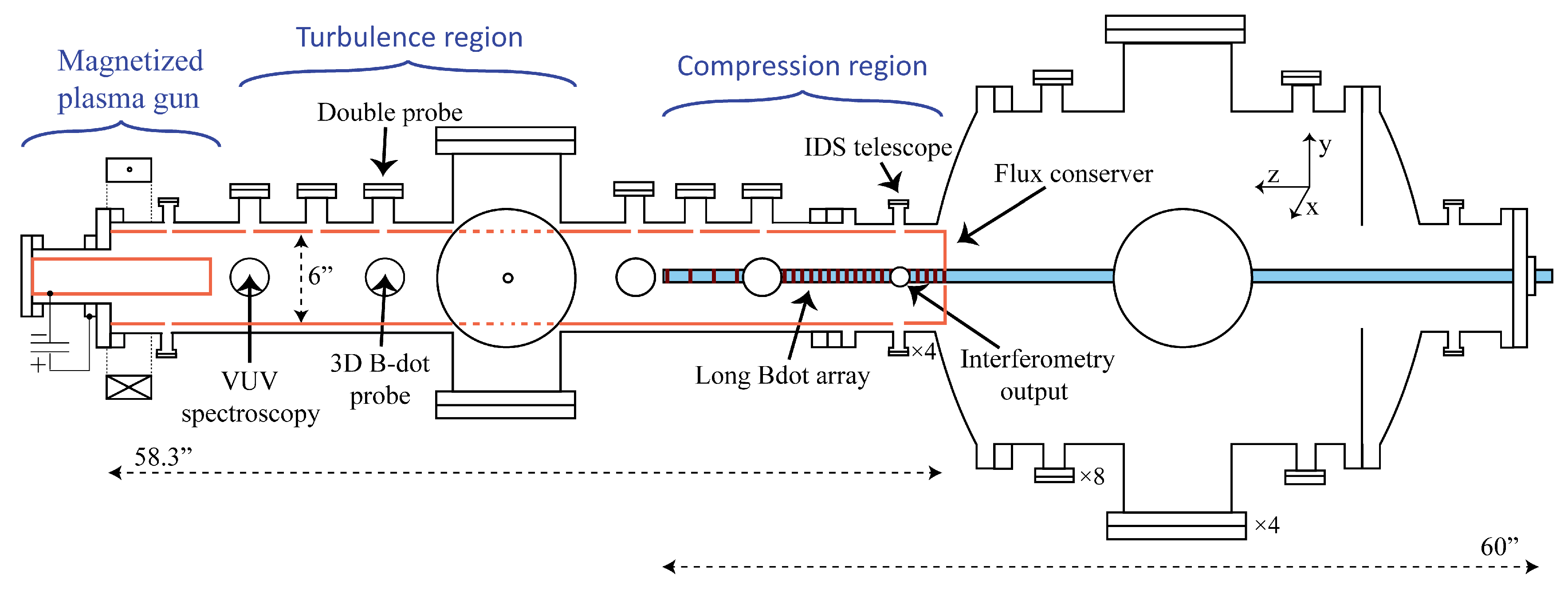
2. SSX Plasma Wind Tunnel

2.1. SSX Device

Over the past two decades, the Swarthmore Spheromak Experiment (SSX) has been used in many different configurations for the study of several interesting phenomena, such as magnetic reconnection [13] and self-organization [11,12], MHD turbulence [8], and magnetothermodynamics [14,15]. In the present configuration, the SSX device features a 1.5 m-long high-vacuum chamber in which we generate n e 10 15 cm 3 , T i 20 eV, B 0.5 T hydrogen plasmas (See Figure 1). The entire set-up is divided into three main sections: (i) plasma source region, (ii) turbulence region, and (iii) compression region. In the first region, a magnetized coaxial plasma gun is installed which generates fully ionized, magnetized plasma.
Plasma is accelerated to high velocity ( 50 km/s) by J × B force in the gun with discharge currents up to 100 kA, and are injected into a highly evacuated, field-free, cylindrical target volume. For these studies, the cylinder is highly elongated ( / r 20 ). The volume is bounded by a highly conducting copper shell ( r = 0.08 m, thickness 3 mm). The inner, plasma-facing surface of the flux conserver is coated with tungsten.
The plasma ejected out of the gun is tilt-unstable and relaxes to a twisted magnetic structure. We use the initial relaxation phase to study MHD turbulence, though this work focuses on the fully-formed plasma object. Parameters match those of earlier studies in which the magnetic structure of the object was confirmed by detailed measurements [11,12]. We use an axially-oriented B ˙ probe array to measure magnetic field structure in this study, and find that it is consistent with the previous observations. The plasma evolves to an equilibrium that is well described by a non-axisymmetric, force-free state (Taylor state) despite finite plasma pressure ( β 20 % ).
We used vacuum ultraviolet (VUV) spectroscopy as well as a swept double-Langmuir probe for T e measurements. The VUV spectroscope is installed 5 cm away from the gun (in the turbulence region) and is integrated over a diametric line of sight. In the same region at 25 cm away from the gun, a double Langmuir probe (at the center) and a co-located B ˙ probe (radially 1 cm away from the center) are installed to measure local T e , plasma density ( n e ), and three orthogonal components of the magnetic field (B). A time trace from these probes is shown in Figure 2.
Ion temperatures are measured at the far end of the flux conserver (124 cm away from the gun) using an ion Doppler spectroscopy (IDS) system with a 1 MHz cadence [16]. Since our hydrogen plasmas are close to full ionization, we measure emission from C I I I impurity ions. Light from the C I I I 229.687 nm line collected from the plasma along a chord is dispersed to 25th order on an echelle grating and is recorded using a 16-channel PMT. The time-resolved proton temperature and line-of-sight average velocity are inferred from the observed thermal broadening and Doppler shift of the emission line, respectively. The line-of-sight is across the flow direction and is located near the end wall of the flux conserver where the plasma stagnates. We measure a line-averaged plasma density at the same axial location using a HeNe laser interferometer (orthogonal sight line). A time trace of the measured average density is shown in Figure 3.

2.2. Taylor States

Relaxed “Taylor” states are minimum energy states of magnetohydrodynamics under the constraint of conserved global magnetic helicity. Taylor-state fields obey the force-free eigenvalue condition: × B = λ B [9,10]. The eigenvalue, λ , describes the pitch of the resulting helical state, and is related to the inductance of the plasma.
Ampere’s law shows that the current density and magnetic field are parallel (“force-free” indicates the lack of J × B forces):
λ B = × B = μ 0 J .
Integrating both sides over an appropriate surface gives:
λ B · d A = μ 0 J · d A λ Φ = μ 0 I ,
where Φ is the magnetic flux through the surface and I is the total current flowing through the surface. Since the inductance is defined by the ratio Φ / I , we have a simple model for the inductance of the relaxed plasma: L = μ 0 / λ . Plasma objects relaxing to Taylor states seek the minimum λ , which is equivalent to maximizing their inductance.
An upper bound on the lifetime of a force-free equilibrium can be estimated by calculating the L / R time for the decay of the plasma current. Roughly, the resistance is the resistivity η times some length, divided by some area. So, R has the units of η / or λ η , since the characteristic length scale of the Taylor state is defined by its eigenvalue. This suggests a compact formula for estimating the lifetime:
τ = L R = μ 0 λ 2 η .
This time scale can also be obtained directly from the induction equation with a simple application of Ohm’s Law:
d B d t = η μ 0 2 B + × v × B .
In the limit of negligible flow (appropriate for a quasi-static equilibrium), this reduces to:
d B d t = η μ 0 2 B η λ 2 μ 0 B ,
giving the same estimate for the timescale of the plasma decay. Using Spitzer resistivity and T e = 7 eV, we predict τ 30 μ s for our plasma. Note that all non-ohmic energy losses are neglected in this model.

2.3. Equilibration of Proton and Electron Temperatures
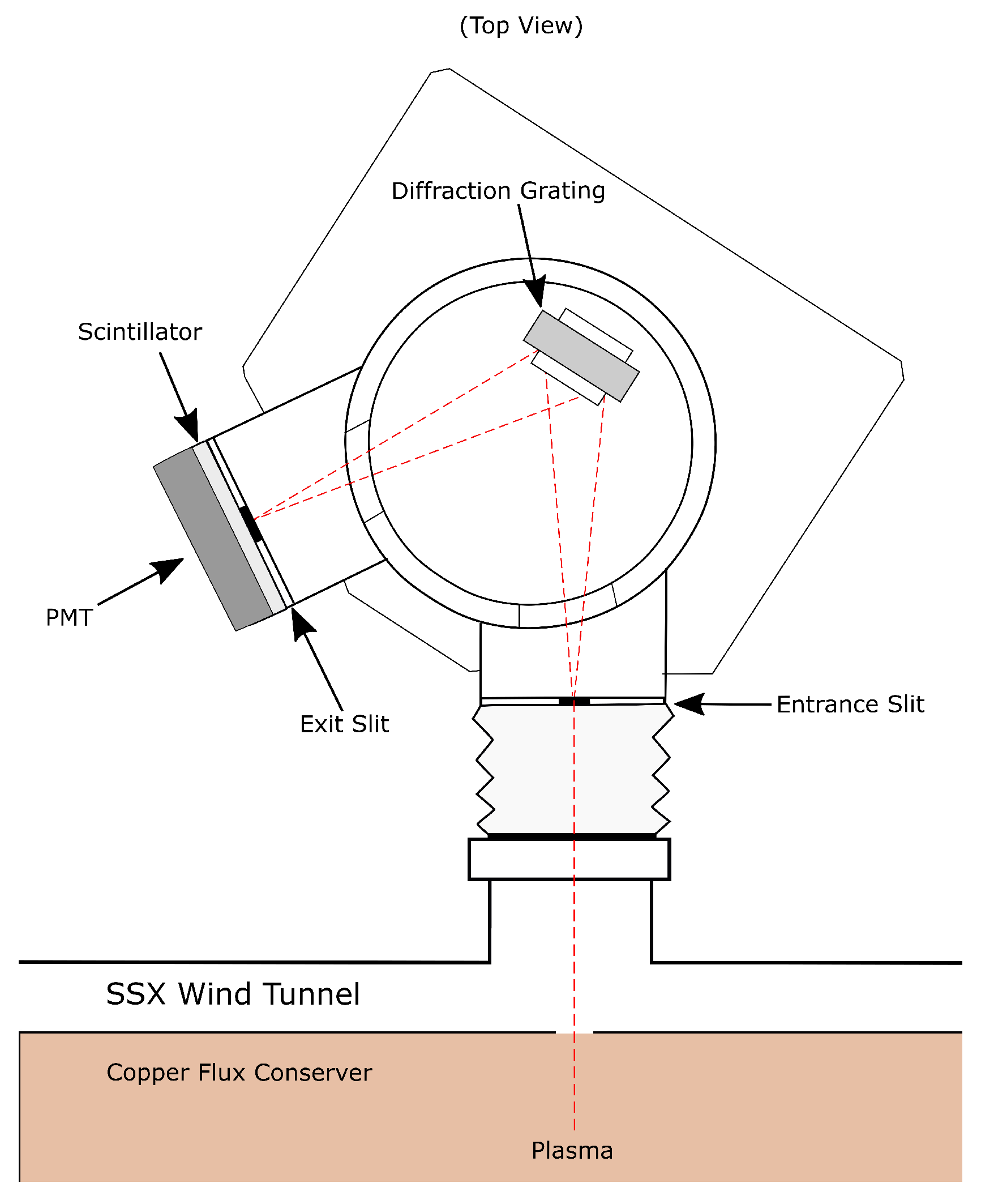
As is typical in compact toroids, T i > T e in the initial plasma formed by the coaxial gun. In order to gain insight into the limitations on the plasma lifetime, we hope to identify the dominant energy channels for dissipation after the equilibrium is formed. As a first step, we measure time-resolved electron and impurity ion temperatures and compare their behavior with a simple model.
We expect that over the lifetime of the plasma, the warm proton component will cool due to collisions with the electrons. This can be modeled with a simple Newton cooling-type equation:
d T p d t = ν p e ( T e T p ) ,
where T p is the proton temperature and T e is the electron temperature. The proton–electron equilibration rate [17] can be written as:
ν p e = 3.24 × 10 9 n e l n Λ ( T e + T i / 1836 ) 3 / 2 ,
where l n Λ is the Coulomb logarithm, temperatures are measured in eV, and densities in cm 3 . Since the impurity concentration in SSX plasma is very low (≲1%) and the electron temperatures are on the order of 10 eV, we assume that the effective charge in the bulk plasma is Z e f f = 1 .
The experimental results indicate a nearly constant electron temperature, consistent with high electron thermal conductivity. With this in mind, and assuming T e and T p are not too different, thermal equilibration times estimated using this formula are several μ s ( T e = 10 eV, n e 10 15 cm 3 , and l n Λ = 8.4 ).

3. VUV Spectroscopy

3.1. Background

The first vacuum ultraviolet (VUV) spectrograph was built by Schumann in 1893 [18]. In the decades since then, the accuracy and ability to measure radiation in the ultraviolet region (the range from 210 nm down to about 1 nm) has increased dramatically [18]. Given that both glass and air are opaque in this region, the measurements—including the transport, diffraction, and detection of UV photons—must be performed either under vacuum, or in a gas that is transparent in the ultraviolet region. Although spectroscopy has the disadvantage of making line-averaged rather than localized measurements, it is noninvasive and does not perturb the plasma.
In our experiment, the ultraviolet radiation emitted by the plasma is transmitted under vacuum to our VUV monochromator, where the photons strike a magnesium-fluoride coated diffraction grating, then pass into a a sodium salicylate scintillator which fluoresces at 420 nm. The 420 nm photons pass through a glass vacuum port and are detected by a photomultiplier tube (PMT), which produces a trace of the diffracted line intensity versus time [19].

3.2. SSX VUV System

We measured the electron temperature along a 0.16 m chord by taking the ratio of C I I I 97.7 nm ( 1 P 1 1 S 0 ) to C I V 155 nm ( 2 P 1 / 2.3 / 2 2 S 1 / 2 ) line intensities [20] using a McPherson 234 M8 0.2 m vacuum ultraviolet monochromator (see Figure 4). Both the entrance and exit slits of the monochromator are adjustable. The entrance slit controls the number of photons entering the monochromator, while the exit slit can be used to control the spectral resolution.
We used a 1200/mm grating so the dispersion of our 0.2 m monochromator was
Δ λ λ = s i n θ 1 / 1200 m m 200 m m = 4 n m / m m .
Resolution is dispersion times detector size, so
R = 4 n m / m m × 0.125 m m = 0.5 n m
if we use 125 μ m exit slits. This is the optimum resolution of our monochromator.
We previously developed a calibration curve for the VUV monochromator at visible wavelengths [20]. During SSX experiments, we are able to scan through the 97.7 nm and 155 nm lines to ensure we are at the center wavelength, and confirm the original calibration. The M g F 2 -coated aluminum grating (1200/mm) does not have flat efficiency over this wavelength range (Figure 5). The grating efficiency differs by a factor of 3 for the 97.7 nm and 155 nm lines.
The C I I I and C I V line intensities have different temperature dependences. Using the measured density of the plasma (Figure 3), we can reconstruct the electron temperature by using the measured ratio of C I I I 97.7 nm and C I V 155 nm line intensities. This data was calculated using a non-LTE excitation kinematics code (PrismSPECT) at several densities and temperatures and interpolated smoothly between calculated points [20] (Figure 6). The corrected photocurrents were smoothed over a 0.25 μ s window, and standard error was calculated. Then, the line ratio at each point in time was converted into an electron temperature, using Figure 6.
In Figure 7 we present the corrected photocurrent for both C I I I 97.7 nm and C I V 155 nm. Approximately 10 shots were averaged to obtain a good average with acceptable errors. In Figure 8, we present T e ( t ) for the data in Figure 7, using Figure 6 and a fixed density of 5 × 10 15 cm 3 (see Figure 3) to project the line ratio to a temperature as a function of time. Errors were propagated in the standard way.

4. Double Langmuir Probe

Local plasma density and electron temperature measurements were performed using a double Langmuir probe (DLP) [21]. A time series of ion saturation current from a DLP is a good proxy for electron density (see Figure 2). In the past, we used a double probe on the SSX MHD wind tunnel to measure radial profiles of electron density and temperature, as well as local density fluctuations [8].
A useful aspect of a double Langmuir probe with identical electrodes is that the I–V characteristic is symmetric. Since the entire circuit floats with the plasma, and if no potential difference is applied between the electrodes, the circuit will not extract any net current, that is, I ( V = 0 ) = 0 (provided the plasma is quiescent). Furthermore, in a double probe circuit, the maximum current is limited by the ion flux. Therefore, the I-V characteristic has the form [21]:
I ( V ) = I s a t tanh e V 2 T e ,
where the maximum current is given by:
I s a t = n e e A c s , i .
Here c s , i is the ion sound speed and is given by T e M i . Hence, the full expression can be written as:
I ( V ) = n e e A T e M i tanh e V 2 T e .
The SSX double Langmuir probe consists of two 1.5 mm diameter tungsten wires. The tungsten wires are installed in an alumina tube closed at the plasma-facing end and cut from the sides so that only a nearly planar area of the probes is exposed to the plasma. The exposed probe areas are 1.5 mm long and 0.8 mm wide. The probe separation is about 3 mm. Probe tips are oriented across the flow direction to prevent one probe tip from shadowing the other.
The probe tips are biased using a 360 μ F capacitor bank charged with an external power supply that is isolated during the plasma discharge to prevent any ground loops. The voltage droop is typically less than 10 % after a discharge, so the voltage between the probe tips is nearly constant. The dynamical voltage difference between the probe tips is monitored using a Tektronix isolated voltage probe during a shot. A high-bandwidth (100 MHz) current transformer (Tektronix TCP312A probe) reports the ion current flowing between the probe tips. Typical ion current magnitudes were ≤20 A, consistent with I = n e c s , i A , and calibrated with a HeNe laser interferometer [8,22].
The biasing voltage between the probe tips was scanned from −60 V to +60 V with a 5 V interval, and 10 shots of the wind tunnel were recorded at each biasing voltage. One such scan is shown in Figure 9 at 100 μ s. Electron temperature and density were extracted from the double probe data at each time step using Equation (3). The fit yielded T e = 9.7 eV with ≈12% error and n e = 1.7 × 10 14 cm 3 at 100 μ s. We suspect that the DLP was over-estimating T e (see Figure 8) but under-estimating density (see Figure 3) at 100 μ s. Nonetheless, we will continue to use it as a proxy for local density.

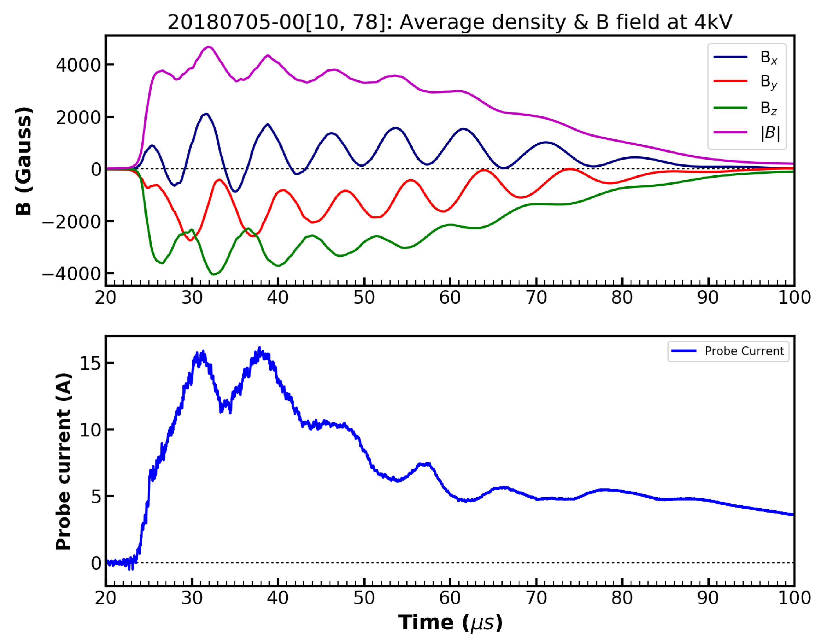
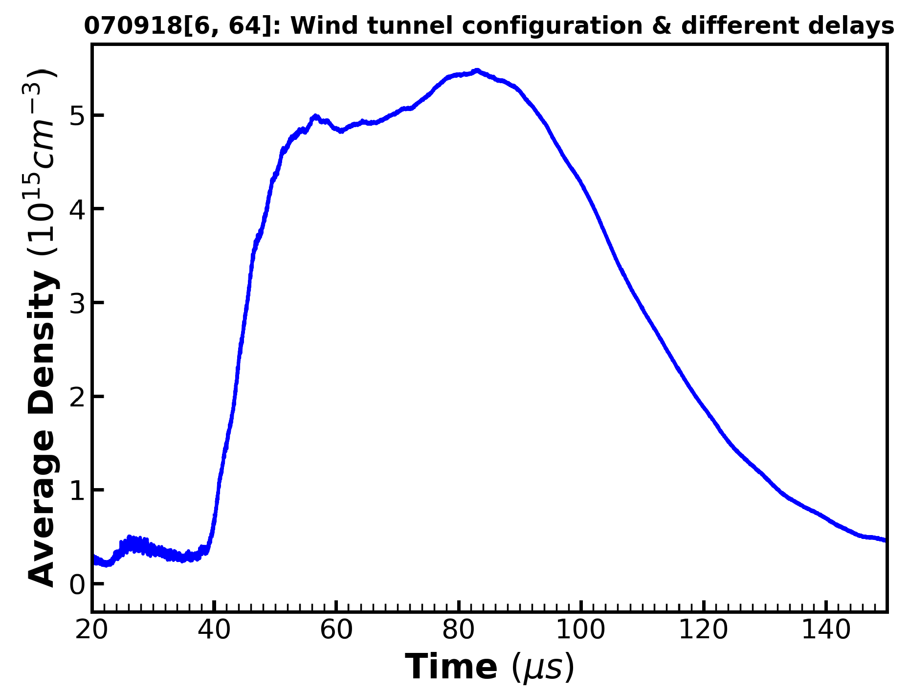
5. Experiment and Results

In Section 3.2 we found that our electron temperature was about 7 eV for most of the discharge. Using our model (Equation (1) ), we could calculate an e-folding lifetime of τ = μ 0 λ 2 η = 29 μ s. In Figure 10, we show the average magnetic field | B | as a function of time. If we extracted an e-folding time as the Taylor state began to decay, we found τ = 30 μ s. Later in time, the decay was faster ( τ = 14 μ s).
We found that the proton temperature in SSX was initially always higher than T e , consistent with expectations for a magnetized coaxial gun (Marshall gun). In Figure 11, we show the cooling of warm protons (measured downstream of the gun) and superpose our T e result. Although they were measured at different locations (124 cm away from the gun for the protons, 5 cm for the electrons), we did not expect gradients in T e along field lines. Since electron heat flux was approximately Q e 0.71 n k T e v and v 1 m/ μ s, the electrons were in local thermal equilibrium during the 100 μ s evolution of the experiment. From our model (Equation (2)), we calculated an e-folding cooling time of ∼1 μ s (using n e = 5 × 10 15 and 7 eV). Evidently, other effects were preventing the protons from cooling rapidly. We suspect that energy from the MHD cascade during turbulent relaxation ultimately put heat into the ion component [23].
The ion temperature dropped below the electron temperature after ∼65 μ s, but this does not preclude ion–electron collisions as the primary cooling channel for ions. The ohmic power dissipated during the decay of the magnetic fields preferentially heats electrons [24,25]. It is possible that the electron transport rate controls the evolution of the plasma late in time. If this is true, the steepening of the decay in the magnetic field after the time at which the protons cool below the electron temperature may be due to the exhaustion of the proton heat flux into the electrons. Protons continue to transfer heat to electrons, but at a reduced rate, while the electron temperature is maintained by the decay-induced current.

6. Discussion and Summary

High ion temperature is an obvious requirement for practical fusion energy, since fusion cross sections peak at temperatures over 10 keV. In addition, the Lawson criterion requires density, temperature, and confinement time such that n T τ 10 21 keV s m 3 . The agreement between our inductive/Spitzer decay model and the initial decay of the plasma suggests that the lifetime is indeed dependent on the electron temperature, and that it in turn needs to be high to enable success in MIF experiments. However, our results in Section 5 indicate that the ion cooling rate was slower than the electron–ion collision rate suggests. It is possible that improved MIF targets could be produced with higher ion temperatures and moderate electron temperatures. We do not yet have a model for what sets the electron temperature for the Taylor state equilibrium. An explanation of why it remains nearly constant throughout the evolution of the plasma could illuminate the contributions of various loss channels.
As we continue our experiments, we have increased our focus on the cleanliness of the vacuum. Figure 12 shows a typical visible spectrum of hydrogen plasma. We observe multiple hydrogen lines, as expected, in addition to an impurity line ( 501 nm). We use a meticulous process for cleaning the vacuum walls of the SSX involving baking the stainless steel vacuum chamber to 250 C and running a Helium glow discharge in the wind tunnel section. We hope to glean information about the importance of impurities for electron heating and cooling by improving the vacuum conditions.
In an effort to explore the confinement properties in more detail, we are currently simulating particle orbits in the Taylor state equilibrium fields. We solve the force-free equation for the lowest eigenvalue in our particular geometry and track particle orbits in the resulting field. Preliminary results seem to indicate that flux surfaces may form in parts of the Taylor state. More work is needed to map out the particle confinement in enough detail to inform the question of a static electron temperature.

Author Contributions

All authors have contributed to the manuscript. M.K. (the lead author, and SSX experiment operator) built and operated the double Langmuir probe and the magnetic probes, and analyzed the data obtained from the above-mentioned probes and ion Doppler spectroscopy & interferometry for carrying out the studies presented in this paper. K.G. (the second author) calibrated and operated the VUV spectrometer, and analyzed the obtained data. M.K. and K.G. drafted the manuscript and designed the figures. A.D.L. and M.R.B. (the SSX Principal Investigator) revised the draft and contributed to the writing.

Funding

This work was supported by the DOE Advanced Projects Research Agency (ARPA) ALPHA program project DE-AR0000564.

Acknowledgments

The authors wish to acknowledge the support and encouragement of ARPA program manager Patrick McGrath. Technical support from Steve Palmer and Paul Jacobs at Swarthmore for SSX is also gratefully acknowledged.

Conflicts of Interest

The authors declare no conflict of interest.

References

  1. Lindemuth, I.R.; Reinovsky, R.E.; Chrien, R.E.; Christian, J.M.; Ekdahl, C.A.; Goforth, J.H.; Haight, R.C.; Idzorek, G.; King, N.S.; Kirkpatrick, R.C.; et al. Target Plasma Formation for Magnetic Compression/ Magnetized Target Fusion. Phys. Rev. Lett. 1995, 75, 1953. [Google Scholar] [CrossRef] [PubMed]
  2. Binderbauer, M.W.; Guo, H.Y.; Tuszewski, M.; Putvinski, S.; Sevier, L.; Barnes, D.; Rostoker, N.; Anderson, M.G.; Andow, R.; Bonelli, L.; et al. Dynamic Formation of a Hot Field Reversed Configuration with Improved Confinement by Supersonic Merging of Two Colliding High β Compact Toroids. Phys. Rev. Lett. 2010, 105, 045003. [Google Scholar] [CrossRef] [PubMed]
  3. Degnan, J.H.; Amdahl, D.J.; Domonkos, M.; Lehr, F.M.; Grabowski, C.; Robinson, P.R.; Ruden, E.L.; White, W.M.; Wurden, G.A.; Intrator, T.P.; et al. Recent magneto-inertial fusion experiments on the field reversed configuration heating experiment. Nucl. Fusion 2013, 53, 093003. [Google Scholar] [CrossRef]
  4. Wurden, G.A.; Hsu, S.C.; Intrator, T.P.; Grabowski, T.C.; Degnan, J.H.; Domonkos, M.; Turchi, P.J.; Campbell, E.M.; Sinars, D.B.; Herrmann, M.C.; et al. Magneto-Inertial Fusion. J. Fusion Energy 2016, 35, 69–77. [Google Scholar] [CrossRef]
  5. Peacock, N.J.; Robinson, D.C.; Forrest, M.J.; Wilcock, P.D.; Sannikov, V.V. Measurement of the Electron Temperature by Thomson Scattering in Tokamak T3. Nature 1969, 224, 488. [Google Scholar] [CrossRef]
  6. Laberge, M. Experimental Results for an Acoustic Driver for MTF. J. Fusion Energy 2009, 28, 179–182. [Google Scholar] [CrossRef]
  7. Brown, M.R.; Schaffner, D.A. SSX MHD plasma wind tunnel. J. Plasma Phys. 2015, 81. [Google Scholar] [CrossRef]
  8. Brown, M.R.; Schaffner, D.A. Laboratory sources of turbulent plasma: A unique MHD plasma wind tunnel. Plasma Sour. Sci. Technol. 2014, 23, 063001. [Google Scholar] [CrossRef]
  9. Taylor, J.B. Relaxation of Toroidal Plasma and Generation of Reverse Magnetic Fields. Phys. Rev. Lett. 1974, 33, 1139. [Google Scholar] [CrossRef]
  10. Taylor, J.B. Relaxation and magnetic reconnection in plasmas. Rev. Mod. Phys. 1986, 58, 741. [Google Scholar] [CrossRef]
  11. Gray, T.; Brown, M.R.; Dandurand, D. Observation of a Relaxed Plasma State in a Quasi-Infinite Cylinder. Phys. Rev. Lett. 2013, 110, 085002. [Google Scholar] [CrossRef] [PubMed]
  12. Cothran, C.D.; Brown, M.R.; Gray, T.; Schaffer, M.J.; Marklin, G. Observation of a Helical Self-Organized State in a Compact Toroidal Plasma. Phys. Rev. Lett. 2009, 103, 215002. [Google Scholar] [CrossRef] [PubMed]
  13. Cothran, C.D.; Landreman, M.; Brown, M.R.; Matthaeus, W.H. Three-dimensional structure of magnetic reconnection in a laboratory plasma. Geophys. Res. Lett. 2003, 30, 1213. [Google Scholar] [CrossRef]
  14. Kaur, M.; Barbano, L.J.; Suen-Lewis, E.M.; Shrock, J.E.; Light, A.D.; Brown, M.R.; Schaffner, D.A. Measuring the equations of state in a relaxed magnetohydrodynamic plasma. Phys. Rev. E 2018, 97, 011202. [Google Scholar] [CrossRef] [PubMed] [Green Version]
  15. Kaur, M.; Barbano, L.; Suen-Lewis, E.; Shrock, J.; Light, A.; Schaffner, D.A.; Brown, M.R.; Woodruff, S.; Meyer, T. Magnetothermodynamics: Measurements of the thermodynamic properties in a relaxed magnetohydrodynamic plasma. J. Plasma Phys. 2018, 84, 905840114. [Google Scholar] [CrossRef]
  16. Cothran, C.D.; Fung, J.; Brown, M.R.; Schaffer, M.J. Fast, High Resolution Echelle Spectroscopy of a Laboratory Plasma. Rev. Sci. Instrum. 2006, 77, 063504. [Google Scholar] [CrossRef]
  17. Huba, J.D. NRL Plasma Formulary; Office of Naval Research: Arlington, VA, USA, 2013. [Google Scholar]
  18. Milazzo, G.; Cecchetti, G. Vacuum Ultraviolet Spectroscopy. Appl. Spectrosc. 1969, 23, 197–203. [Google Scholar] [CrossRef]
  19. Details at the McPherson. Available online: http://mcphersoninc.com/ (accessed on 4 May 2018).
  20. Chaplin, V.H.; Brown, M.R.; Cohen, D.H.; Gray, T.; Cothran, C.D. Spectroscopic Measurements of Temperature and Plasma Impurity Concentration during Magnetic Reconnection at the Swarthmore Spheromak Experiment. Phys. Plasmas 2009, 16, 042505. [Google Scholar] [CrossRef]
  21. Johnson, E.O.; Malter, L. A Floating Double Probe Method for Measurements in Gas Discharges. Phys. Rev. 1950, 80, 58. [Google Scholar] [CrossRef]
  22. Buchenauer, C.J.; Jacobson, A.R. Quadrature interferometer for plasma density measurements. Rev. Sci. Instrum. 1977, 48, 769–774. [Google Scholar] [CrossRef]
  23. Maruca, B.A.; Kasper, J.C.; Bale, S.D. What Are the Relative Roles of Heating and Cooling in Generating Solar Wind Temperature Anisotropies? Phys. Rev. Lett. 2011, 107, 201101. [Google Scholar] [CrossRef] [PubMed]
  24. Jarboe, T.R.; Barnes, C.W.; Henins, I.; Hoida, H.W.; Knox, S.O.; Linford, R.K.; Sherwood, A.R. The Ohmic heating of a spheromak to 100 eV. Phys. Fluids 1984, 27, 13–15. [Google Scholar] [CrossRef]
  25. Wysocki, F.J.; Fernández, J.C.; Henins, I.; Jarboe, T.R.; Marklin, G.J. Evidence for a Pressure-Driven Instability in the CTX Spheromak. Phys. Rev. Lett. 1988, 61, 2457. [Google Scholar] [CrossRef] [PubMed]
Figure 1. Schematic of the Swarthmore Spheromak Experiment (SSX) device in the wind tunnel configuration. The entire device is divided into three main sections: (i) plasma source region, (ii) turbulence studies region, and (iii) compression region. In the first region, a magnetized coaxial plasma gun is installed which generates fully ionized, magnetized plasma. In the turbulence region, vacuum ultraviolet (VUV) spectroscopy is installed 5 cm away from the source for T e measurements. In the same region at 25 cm away from the gun, a double Langmuir probe and a co-located B ˙ probe are installed to measure T e , n, and three orthogonal components of the magnetic field. In the compression region, a long B ˙ probe array is aligned axially to measure magnetic field structure and time of flight velocity. In addition, ion Doppler spectroscopy (IDS) and HeNe laser interferometry are used for measuring the ion temperature and plasma density, respectively, at a distance of 124 cm from the gun.
Plasma 01 00020 g001
Figure 2. Typical SSX wind tunnel data. (top) Magnetic field (three components and | B | ); (bottom) double Langmuir probe ion saturation current. Magnetic field data are a 69-shot ensemble average. Measurement was made at the location shown in Figure 1.
Plasma 01 00020 g002
Figure 3. Time trace of average electron density obtained from HeNe laser interferometry measured 124 cm away from the gun from 58 plasma shots.
Plasma 01 00020 g003
Figure 4. Schematic of the VUV monochromator. Radiation emitted by the plasma passes thought a hole in the copper flux conserver, then though a flange into the monochromator, all under vacuum. The diffraction grating selects and refocuses a narrow band of light centered at a selected wavelength. The photons strike a scintillator, which fluoresces and the signal is detected and amplified by the photomultiplier tube (PMT).
Plasma 01 00020 g004
Figure 5. Grating efficiency of McPherson 1200 grooves/mm A l + M g F 2 grating. We operated at 97 nm and 155 nm, where the grating efficiency differs by a factor of 3.
Plasma 01 00020 g005
Figure 6. Calibration curve. Intensity ratio of the 97.7 nm C I I I to the 155 nm C I V as a function of T e in electron volts, at two densities. Ratios were calculated using a non-LTE excitation kinematics code (PrismSpec) at several densities and temperatures and interpolated between [20].
Plasma 01 00020 g006
Figure 7. Typical photocurrent measured at (top) 97.7 nm and (bottom) 155 nm using VUV spectroscopy. The 97.7 nm line corresponds to C I I I transitions (14-shot average) and the 155 nm line corresponds to C I V transitions (8-shot average). Error bars reflect the standard error. We divided the 97 nm signal by the 155 nm signal to measure T e .
Plasma 01 00020 g007
Figure 8. Electron temperature. T e was measured by averaging the ratio between the intensities of CIII and CIV photons, and then converted to temperature using the calibration curve, assuming a density of 5 × 10 15 on Figure 6. Error bars were propagated from Figure 7.
Plasma 01 00020 g008
Figure 9. Typical I–V curve of a double probe obtained using ∼140 SSX shots. This data was taken at 100 μ s and averaged over a 10 μ s window. Data was fit to the tanh function Equation (3), and error in the temperature was ≈12%. The upper panel shows that at high bias voltages, secondary emission masked the probe characteristics. The lower panel is the data selected for the fit to obtain electron temperature.
Plasma 01 00020 g009
Figure 10. Time trace of average magnetic field | B | obtained from the small B ˙ probe, at 25 cm away from the gun, measuring three orthogonal components of the magnetic field. The average is obtained using 63 shots taken under similar conditions. The average magnetic field shows an e-folding time of 30 μ s (shown by the black straight line) at earlier time, whereas at later time, the e-folding time was around 14 μ s (shown by the blue straight line).
Plasma 01 00020 g010
Figure 11. Time trace of average ion temperature (measured using ion Doppler spectroscopy, 124 cm away from the gun) and electron temperature obtained from VUV spectroscopy measured 5 cm away from the gun.
Plasma 01 00020 g011
Figure 12. Visible spectrum produced by our Ocean Optics Spectrometer, with the strongest lines labeled with the most likely atomic source. Multiple hydrogen lines are present—including H α at 656 nm, H β at 486 nm, and H γ at 434 nm. In addition to these lines, one more line is present around 501 nm, which indicates that our plasma was contaminated by some impurities.
Plasma 01 00020 g012

