
Determination of Highly Transient Electric Field in Water Using the Kerr Effect with Picosecond Resolution


Institute of Plasma Physics of the Czech Academy of Sciences, U Slovanky 2525/1a, 182 00 Prague, Czech Republic
*
Authors to whom correspondence should be addressed.
Plasma 2024, 7(2), 316-328; https://doi.org/10.3390/plasma7020018
Submission received: 20 March 2024
/
Revised: 12 April 2024
/
Accepted: 17 April 2024
/
Published: 22 April 2024
Abstract
:This study utilizes the Kerr effect in the analysis of a pulsed electric field (intensity ~108 V/m, limited by the liquid dielectric strength) in deionized water at the sub-nanosecond time scale. The results provide information about voltage waveforms at the field-producing anode (160 kV peak, du/dt > 70 kV/ns). The analysis is based on detecting the phase shifts between measured and reference pulsed laser beams (pulse width, 35 ps; wavelength, 532 nm) using a Mach–Zehnder interferometer. The signal-to-noise ratio of the detected phase shift is maximized by an appropriate geometry of the field-producing anode, which creates a correctly oriented strong electric field along the interaction path and simultaneously does not electrically load the feeding transmission line. The described method has a spatial resolution of ~1 μm, and its time resolution is determined by the laser pulse duration.
1. Introduction
Electric discharges in liquids are intensively studied from the point of view of the fundamental processes leading to plasma generation in a liquid environment and because of their application potential in various areas [1,2]. One category of plasma sources is based on using nanosecond high-voltage (HV) pulses together with electrode geometries, enabling the generation of ultra-high electric fields that can disrupt the H-bonded structure of liquid water [3]. Under such extreme conditions, elongated nanocavities are supposed to form, in which the conditions are suitable for the avalanche multiplication of charged species with the subsequent formation of a highly non-equilibrium plasma [4,5].
In our recent study [6], we showed that a nanosecond discharge in carefully degassed and deionized water developed in two distinct phases. The initial (so-called dark) phase was characterized by a significant disturbance of the refractive index of water near the high-voltage electrode and precedes the following (so-called luminous) phase characterized by a weak emission continuum in the visible–NIR spectral range. We further demonstrated that after observing the first dark discharge structures (evidencing local refractive index changes), approximately 600–800 ps (depending on the high-voltage amplitude) was required to detect the first photons, thus revealing the onset of the luminous phase. While the initial changes in refractive index are thought to be due to the formation of nanovoids in the electrostricted polar liquid, the observation of the visible–NIR photons is likely due to the multiplication and acceleration of energetic electrons inside the nanovoids, which lose energy through bremsstrahlung. The potential association of nanovoid formation with the local value of the electric field strength thus appears to be a rather important point (along with other points such as the detection of the nanovoids themselves) that needs to be resolved to prove the electrostriction-based concept of the discharge initiation mechanism. To verify and understand the essence of such discharges, it is necessary to use state-of-the-art diagnostics that provide specific information about driving processes with ultra-high spatio-temporal resolution.
It is necessary to analyze pulsed electric fields in water at the sub-nanosecond time scale to understand their physical properties. The measurement of in situ electric fields implementing the Kerr effect has been utilized for various high-voltage power supplies. Pulsed electric fields were analyzed by Novac [7,8], who used Malus’ law to determine the Kerr constant of water. Minamitani et al. [9] utilized a Mach–Zehnder interferometer to determine the spatial and temporal variation in the electric field applied in pin-to-plane electrode geometry in water. Zahn et al. [10,11] performed the two-dimensional mapping of electric field structures using the Kerr effect. They investigated electric field structures during the breakdown from various electrode geometries immersed in the dielectric liquid. Sarkisov et al. [12] utilized the Kerr effect during the breakdown of water, and they determined the electric field at the tip of the streamer head propagating in the water. They have reported that the measured strength of the electric field at the tip of the streamer is six times higher than that of the applied interelectrode electric field. Similar experiments were performed and described in [13,14,15], in some cases with strong electric fields (5 GV/m), leading to saturation of the liquid polarization. In the case of insulating dielectric liquids, kerrograms were successfully used to analyze the distribution of the injected space charge [16,17].
In this work, we utilized a diagnostic approach based on picosecond laser interferometry and the Kerr effect. Waveforms of the electric field were then compared with the data from an HV capacitive probe.
2. Experimental Setup and Methods
2.1. Experimental Device and Electrical Measurements
The present experiments employ a diagnostic discharge reactor, which was described in more detail in previous works [3,4,6,18]; the device is illustrated in Figure 1. The reactor consists of a stainless-steel body equipped with a coaxial HV interface, a capacitive probe sensor, optical windows, and a working liquid inlet and outlet. A significant difference between the present and previous experiments lies in the shape of the HV electrode. Here, we use a small metal plate as the HV electrode, while in the previous experiments, we used a needle electrode. The plate HV electrode is attached directly to the inner conductor of the coaxial line. The discharge chamber was filled with pre-degassed DI water with a conductivity of ~1.1 μS/cm at 22 °C. In-reactor degassing can be performed if there is a gas bubble adhering to the HV electrode. The HV pulse power generator FPG 150-01 NM6 (FID Technology GmbH, Burbach, Germany) produces positive HV pulses of ~5.5 ns full width at half maximum (FWHM). The HV pulses are fed into the reactor using a 2.8 m long HV coaxial cable, which is unmatched at the opened end. A built-in capacitive probe (CP) (designed by our department) provides a coupling capacitance between the probe electrode and the inner conductor of the cable (approximately 5 × 10⁻¹⁵ F). It is used to monitor HV waveforms near the plate anode (amplitude between 110 and 175 kV). The probe is shunted by a capacitance of 14 pF and loaded with a 93 Ω line, which gives a time constant of 1.3 ns. This means that at the nanosecond time scale, the above-mentioned voltage signal sensed by the probe is significantly influenced by the impulse response of the whole circuit. Therefore, the data recorded by the oscilloscope must be numerically deconvolved to obtain the original waveform.
2.2. Time-Resolved Interferometry
Figure 2 shows a block diagram of the setup used for picosecond laser interferometry with simultaneous detection of the signal from the capacitive probe (CP). The source of the laser pulse is the Katana 05 (Onefive, NKT Photonics, Regensdorf, Switzerland) system (pulse duration, 35 ps; energy, 6.4 nJ; wavelength, 532 nm). The laser beam is first polarized by a polarizer (P), and then it is split by the first beam splitter (BS1) into two perpendicular beams (PB and RB). The probing laser beam (PB) is sent to the measurement chamber (ChM) using a mirror (M1). The analyzer (A) placed in the path of the PB passes only light with polarization selected by the polarizer (P). The reference beam (RB) passes through a delay chamber (ChD), which serves as a phase correction. The electrode area in ChM is magnified by an objective lens (L2), and the same lens (L1) must also be placed in the path of the beam RB to produce correct interferograms at the CCD after merging the beams using the second beam splitter (BS2). Perturbations in the refractive index near the plate anode caused by the Kerr effect are registered as shifts of fringes in interferogram images captured by the camera Canon 760D, 24 Mpx) (Canon, Tokyo, Japan) [4]. Typical interferograms are depicted in Figure 1, where image (c) captures the region of interest without the electric field, and image (d) captures it with the maximum electric field allowed by the dielectric strength of the liquid (i.e., without any discharge event). A digital pulse/delay generator BNC, Model 575 (Berkeley Nucleonics Corp., San Rafael, CA, USA) serves as a trigger and delay source for the synchronization of the HV pulser (FID) with the Katana 05 laser system. The pulse monitor output of the FID produces an input trigger signal for the BNC generator, which produces an input trigger for the Katana 05 laser with the required HV-to-laser pulse delay. However, this synchronization method is affected by jitter on the order of several ns. Therefore, a fast photomultiplier PMT210 (Photek, St Leonards on Sea, UK) detects the part of the laser pulse passing through the BS2, and its output signal is used to monitor the time position of the laser pulse relative to the course of the HV voltage pulse, which is obtained from the CP. Typical CP and PMT waveforms are plotted in Figure 3. The entire experiment is based on multiple acquisitions of interferograms together with the corresponding oscilloscopic records (CP and PMT waveforms) via the DSOX6004A digital oscilloscope (Keysight Technologies, Santa Rosa, CA, USA). The acquisitions are then sorted according to the delay between the CP and PMT waveforms to create a time sequence of interferograms following the evolution of the electric field and are then evaluated.
2.3. Evaluation
The electric field detection in this work is based on the DC Kerr effect defined by the following relationship [19]:
where and are the indices of refraction for light polarized parallel and perpendicular to the direction of the applied electric field E, respectively; is the laser light wavelength in vacuum; and B is the Kerr constant. Values of the Kerr constant were taken from [19] (4.17 × 10⁻¹⁴ m/V2 at 514.5 nm) and [20] (3.21 × 10⁻¹⁴ m/V2 at 546 nm); then, the value at 532 nm was calculated by linear interpolation. This approximation is possible because values of the constant found in different sources are considerably inconsistent anyway [7]. Equation (1) can be solved for the phase shift ϕ between laser beams of parallel and perpendicular polarizations with respect to the direction of the electric field [19], as follows:
where L is the total length of the laser beam path in the area with an electric field.
The shape of the electrode generating electric field is chosen to maximize ϕ for the best possible signal-to-noise ratio. According to Equation (2), this is possible not only by increasing E, which is limited by the liquid dielectric strength and the permittivity saturation [21], but also by increasing L. However, the electrode dimensions are also limited by the electrode self-capacitance, which loads the transmission line, and so it can significantly influence voltage waveforms at the line end. Therefore, electrode geometry was chosen according to Figure 4. In this case, the length of the integration path slightly exceeds 3 mm (which is smaller than the diameter of the inner wire of the cable), and the upper edge is rounded with a radius of 0.25 mm (see also Figure 1c). Such a large radius keeps the electric field just below the critical value at which a discharge could occur in the liquid. The plot in Figure 4 shows the electric field distribution in the y–z plane together with calculated by Equation (1).
This enables us to estimate the phase shift produced by two main areas: just above and near the plate electrode. This is depicted in Figure 5, where the distribution of the electric field lines is also shown with red arrows. As the phase shift depends on E2, the value of the integral in Equation (2) is mainly determined by the field above the electrode and in its close vicinity.
The interaction of a laser beam with a nonlinear medium can be described by the third-order (nonlinear) part of the polarization at a given laser frequency ω [22]. The part of the nonlinear polarization that influences the propagation of the beam is generally calculated using the following equation:
where E(0) is the static electric field, E(ω) is the electric field of the probing laser radiation, χ(3) is the third-order part of the nonlinear susceptibility tensor, ε0 represents the vacuum permittivity, and the factor of 3 is a result of intrinsic symmetries of the tensor in an isotropic medium [22,23]. Although the analyzed electric field is rapidly changing, the bandwidth of its driving voltage pulse falls to the noise level at ~500 MHz (Figure 6). The bandwidth is 6 orders lower than the laser frequency (5.64 × 10¹⁴ Hz) and is safely outside the water dielectric dispersion area and the loss spectrum [24].
For the chosen directions of the electric field and laser polarizations, there are two third-order components of the polarization vector, Px and Py, which are related to the index of refraction n via the susceptibility tensor χ(3):
Here, χ(ef) is an “effective” susceptibility. As n and χ(ef) are field-dependent, they can be written as power series in the following manner:
where second-order terms χ(2), and thus n(2), are omitted in an isotropic medium [22]. This gives the relation between the third-order terms,
and specifically (—z-axis laser polarization and —x-axis laser polarization),
Now, the terms and must be the same in an isotropic medium. Therefore, they vanish in the difference, and finally,
Equation (12) indicates that only the Ez component (see Figure 5) affects the detected phase shift. That means that the proximity of the lateral grounded wall (coaxial line shielding) does not affect the measurements.
The captured interferograms evidence fringe deviation caused by imperfections in the adjustment of the objective lenses and brightness gradient (Figure 7a). These deviations are reproducible in all interferograms captured with the same setup and are, therefore, easily corrected. Figure 7b shows the fringe shift when a strong electric field surrounds the electrode. The fringe shift is evaluated at the apex of the electrode by comparing the fringe position there with its counterpart far from the electrode, where the electric field is negligible. There is a clearly blurred interference pattern aside from the electrode, whose explanation is out of the scope of this study. However, it seems that it has something to do with the rotation of the laser beam polarization [25], which occurs when the beam polarization is neither parallel nor perpendicular to the static electric field. Therefore, in this experiment, the interferometer is set up such that the fringes in the presence of electric field always shift toward the electrode. This ensures that the examined fringe near the electrode apex does not lead across the empty area, and therefore, it can always be paired up with a fringe to the far left of the electrode. Furthermore, due to the electrode symmetry, the electric field at the apex always aims just in the z-direction. Polarizing the laser in the z- or x-direction means that the polarization direction is always either parallel or perpendicular to the electric field in the axis of symmetry, i.e., at the electrode apex.
3. Results and Discussion
The amplitude of the applied voltage at the given pulse width (~5.5 ns FWHM) is limited to roughly 160 kV. Higher amplitudes lead to an almost 100% certainty of triggering a discharge in the liquid. The captured images shown in Figure 8 indicate that the breakdown does not happen during the laser illumination, as the shape of the fringes is apparently uninfluenced by the presence of the plasma filaments. As the filaments are expected to be conductive, they should redistribute the electric field from the electrode surface to their tips. Thus, the fringes should be bent mainly around the tips, which is not the case here. Nevertheless, an analysis of these interferograms is prevented by the imprint of the plasma-induced emission. By inspecting the shape of the fringes (with or without discharge filaments present), we can determine the limit of the HV amplitude below which the formation of luminous filaments does not occur, and thus, there is insufficient formation of the discharge precursors—the nanovoids.
The breakdown threshold can certainly be increased not only by increasing the main electrode radius but also by better polishing the metal surface at the microscale level.
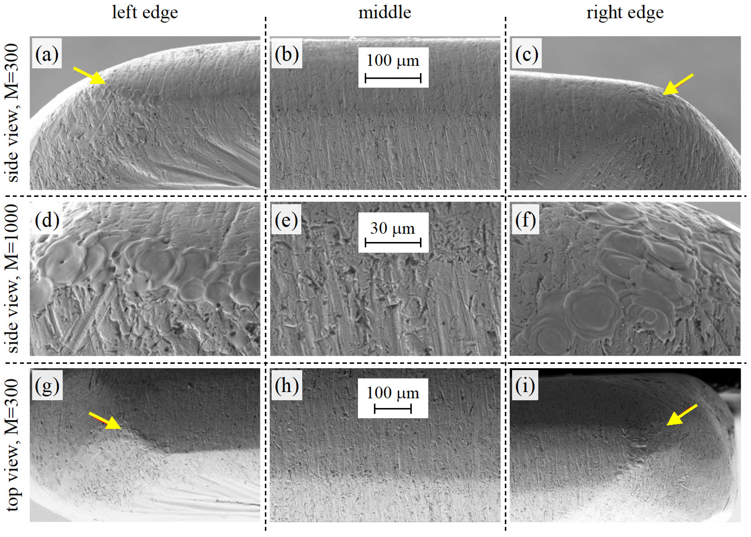
SEM observations of the electrode tip (Figure 9) revealed that in the central area, the tip morphology was intact, and the surface displayed marks (microgrooves) resulting from the original surface preparation and tip shaping by manual grinding. In contrast, at the electrode tip edges, where a secondary rim was formed due to the rounding of the sides of the electrode, a chain of closely packed circular features was observed on top of the original surface. These features had a characteristic diameter between 15 and 25 μm and a smooth surface with wrinkled circumference, indicating local melting of the surface during the discharges followed by shrinking of the molten material. The presence of distinguishable boundaries between the circular features also indicates that they were formed individually during separate pulses. The position of the circular features along the secondary rim with a smaller radius shows that their formation was limited to the area of the greatest electrical potential facilitating plasma (channel) formation. A simulation using the COMSOL Multiphysics software package (version 4.4) shows that it is necessary to deliver energy > 5 × 10⁻⁴ J into the area with a diameter of 20 μm during the voltage pulse (5.5 ns FWHM) to melt the surface of the metal. The corresponding power density is >159 GW/m2.
Figure 10 shows a short series of selected interferograms illustrating the degree of fringe shift at two voltage amplitudes (128 and 160 kV), and both perpendicular (horizontal) and parallel (vertical) laser polarizations with respect to the electric field at the electrode apex (vertical only). For reasons mentioned in Section 2.3, the interferometer is set up in such a way that the fringes always shift downwards, which would otherwise not be the case. The fringe width is adjusted to be much smaller than the electrode apex radius, which enables precise “sampling” of the area.
The evaluated results are plotted in Figure 11. The phase shifts are taken from an area at the anode axis of symmetry, about 20 μm above the anode apex. This distance is much smaller than the apex radius (250 μm). The upper plots correspond to a voltage amplitude of 128 kV, and the bottom plots correspond to an amplitude of 160 kV. The values of the phase shifts (Figure 11a,c) are the opposite of the corresponding laser polarizations, so their absolute values add up after subtraction. The electric field waveforms determined from the phase shifts and the voltage waveforms gained from the signal provided by the capacitive probe are plotted in (Figure 11b,d). It can be clearly seen that the electric field is proportional to the electrode voltage, i.e., only the third-order nonlinearity plays a role here. If there is a decrease in the Kerr constant due to dielectric saturation of the liquid [7,21], it is probably insignificant in an electric field up to 120 MV/m with respect to the achieved measurement error. There is significant noise at low levels of the electric field waveform, and this is the result of noise produced by the CCD in the used camera (noticeable in Figure 7 and Figure 10), which produces an absolute uncertainty of ~1 px in the interferograms. This produces a serious absolute error, especially when the fringe width only measures several px and the fringe shift is very small. Nevertheless, the error is relatively small in a strong electric field (from 2 to 3 ns), where the fringe shift is large. A method utilizing the Hilbert transform [26,27] would likely be more suitable for the phase determination in the interferograms.
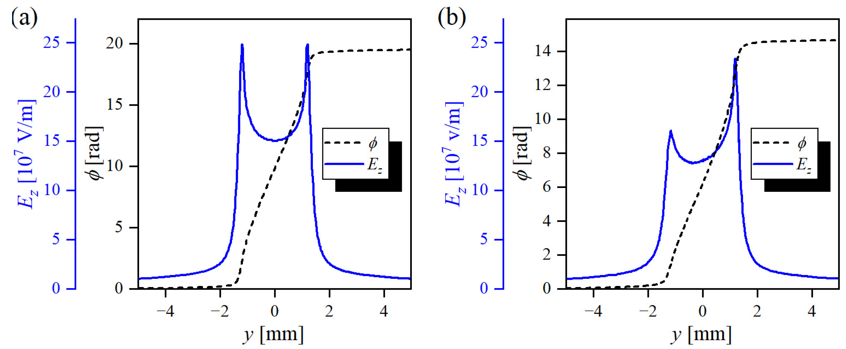
The electric field along the plate anode is not homogeneous (see the plot in Figure 4), and the apparatus detects average <ϕ>, which is proportional to <E2> (Equation (2)). A comparison of the measurements with simulation is performed with an electrode voltage of 160 kV. Figure 12a shows results when the path of the laser beam is perfectly aligned with the electrode apex. In this case, the Ez field component is symmetric around y = 0, and the resulting phase shift calculated by Equation (2) is 19.5 rad, i.e., significantly larger than the one measured at the same voltage (<14.5 rad). The average electric field producing the calculated phase shift results from Equation (2), as follows:
where y1 and y2 delimit the area along the integration path and Ez considerably contributes to the phase shift. In this case, Equation (13) gives E = 157 MV/m, which is also much larger than the measured value (<125 MV/m). There can be several reasons for this discrepancy. First, the real value of the Kerr constant is different from that used in data processing. Second, any imperfections in the electrode shape (hand-made electrode) might lead to a weaker electric field in the experiment. Third, the laser beam might be slightly misaligned. Figure 12b shows Ez along a path, which is elevated at one side of the electrode in the z-direction by 0.25 mm. This type of misalignment might be possible. In this work, we were unable to check the electrode position in the experimental chamber with better precision. The calculated phase shift and electric field are then much closer to the measured values, 14.7 rad and 136 MV/m.
Therefore, this setup is suitable for direct field measurements only if the electrode shape is improved in such a way that the electric field along the electrode apex is homogenized and the path of the probing laser beam is properly aligned with the electrode apex. Furthermore, the exact value of the Kerr constant at 532 nm is not known. Nevertheless, even the described setup can be calibrated by a known signal provided by the capacitive probe. The optical method can then be utilized in cases where the capacitive probe cannot work properly, e.g., when the diagnosed signal is of a very high voltage and large wideband. In that case, it is necessary to place the probe far from the conductor, which limits the probe’s ability to detect wideband signals, as it averages the electric field produced by a long section of the line conductor. This is the area where the described method is excellent. Its time resolution is determined only by the laser pulse duration.
4. Conclusions
In this work, we developed and tested interferometric diagnostics that can be used to systematically investigate the conditions required to produce a nanosecond high-voltage discharge in polar liquids with very high spatio-temporal resolution. In the case of discharge systems based on high-voltage pulses with a rise time of a few nanoseconds and applied to highly curved electrodes, the liquid near the electrode surface was affected by an extremely high electric field, and the initiation of the discharge could be controlled by electrostriction (i.e., by the production of nanoruptures or nanovoids in the liquid).
In this work, it was shown that it is possible to use picosecond laser interferometry to detect phase shifts caused by the Kerr effect and employ it in the analysis of pulsed sub-nanosecond electric fields around properly shaped electrodes immersed in DI water. The analyzed amplitudes of electric fields were of the order of 108 V/m. The maximum rate of increase in the driving voltage was du/dt > 70 kV/ns, and its spectrum fell to a noise level at ~500 MHz. Although the field-producing anode was small enough to not capacitively load the feeding transmission line, a significant phase shift, i.e., signal-to-noise ratio, was detected by the interferometer.
The method was tested for two different voltage amplitudes. In both cases, the electric field was proportional to the electrode voltage, i.e., only the third-order nonlinearity played a role here. As the time resolution of the interferometer is limited only by the laser pulse duration, the method can be utilized in cases where a large voltage amplitude and du/dt prevent the use of capacitive probes. This approach is suitable for a systematic investigation, based on the analysis of interferograms with associated images and oscilloscope recordings, to quantify the threshold conditions necessary to observe discharge initiation (for a given anode curvature and water conductivity). Corresponding experiments are ongoing.
Author Contributions
Conceptualization, P.H., V.P. and M.Š.; Methodology, P.H.; Validation, P.H., V.P., G.A. and M.Š.; Formal analysis, P.H. and G.A.; Investigation, P.H., V.P. and R.M.; Data curation, P.H., V.P. and R.M.; Writing—original draft, P.H.; Writing—review and editing, P.H., V.P., G.A., R.M. and M.Š.; Project administration, M.Š.; Funding acquisition, M.Š. All authors have read and agreed to the published version of the manuscript.
Funding
This research was funded by The Czech Science Foundation, grant number GA24-10903S.
Institutional Review Board Statement
Not applicable.
Informed Consent Statement
Not applicable.
Data Availability Statement
The raw data supporting the conclusions of this article will be made available by the authors upon request.
Conflicts of Interest
The authors declare no conflicts of interest. The funders had no role in the design of the study; in the collection, analyses, or interpretation of data; in the writing of the manuscript; or in the decision to publish the results.
References
- Adamovich, I.; Agarwal, S.; Ahedo, E.; Alves, L.L.; Baalrud, S.; Babaeva, N.; Bogaerts, A.; Bourdon, A.; Bruggeman, P.J.; Canal, C.; et al. The 2022 Plasma Roadmap: Low temperature plasma science and technology. J. Phys. D Appl. Phys. 2022, 55, 373001. [Google Scholar] [CrossRef]
- Joshi, R.P.; Kolb, J.F.; Xiao, S.; Schoenbach, K.H. Aspects of Plasma in Water: Streamer Physics and Applications. Plasma Process. Polym. 2009, 6, 763–777. [Google Scholar] [CrossRef]
- Šimek, M.; Hoffer, P.; Tungli, J.; Prukner, V.; Schmidt, J.; Bílek, P.; Bonaventura, Z. Investigation of the initial phases of nanosecond discharges in liquid water. Plasma Sources Sci. Technol. 2020, 29, 064001. [Google Scholar] [CrossRef]
- Hoffer, P.; Prukner, V.; Schmidt, J.; Šimek, M. Shockwaves evolving on nanosecond timescales around individual micro-discharge filaments in deionised water. J. Phys. D Appl. Phys. 2021, 54, 285202. [Google Scholar] [CrossRef]
- Hoffer, P.; Bílek, P.; Prukner, V.; Bonaventura, Z.; Šimek, M. Dynamics of macro- and micro-bubbles induced by nanosecond discharge in liquid water. Plasma Sources Sci. Technol. 2022, 31, 015005. [Google Scholar] [CrossRef]
- Šimek, M.; Hoffer, P.; Prukner, V.; Schmidt, J. Disentangling dark and luminous phases of nanosecond discharges developing in liquid water. Plasma Sources Sci. Technol. 2020, 29, 095001. [Google Scholar] [CrossRef]
- Novac, B.M.; Banakhr, F.A.; Smith, I.R.; Pecastaing, L.; Ruscassie, R.; De Ferron, A.S.; Pignolet, P. Determination of the Kerr Constant of Water at 658 nm for Pulsed Intense Electric Fields. IEEE Trans. Plasma Sci. 2012, 40, 2480–2490. [Google Scholar] [CrossRef]
- Novac, B.M.; Ruscassie, R.; Wang, M.; De Ferron, A.S.; Pecastaing, L.; Smith, I.R.; Yin, J. Temperature Dependence of Kerr Constant for Water at 658 nm and for Pulsed Intense Electric Fields. IEEE Trans. Plasma Sci. 2016, 44, 963–967. [Google Scholar] [CrossRef]
- Minmitani, S.K.Y.; Minamitani, Y.; Kono, S.; Goan, B.; Kolb, J.; Xiao, S.; Bickes, C.; Lu, X.; Laroussi, M.; Joshi, R.; et al. Nanosecond interferometric measurements of the electric field distribution in pulse charged water gaps. In Proceedings of the Conference Record of the Twenty-Sixth International Power Modulator Symposium, 2004 and 2004 High-Voltage Workshop, San Francisco, CA, USA, 23–26 May 2004; IEEE: Piscataway, NJ, USA, 2004; pp. 516–519. [Google Scholar] [CrossRef]
- Zahn, M.; Takada, T. High voltage electric field and space-charge distributions in highly purified water. J. Appl. Phys. 1983, 54, 4762–4775. [Google Scholar] [CrossRef]
- Zahn, M.; Takada, T.; Voldman, S. Kerr electro-optic field mapping measurements in water using parallel cylindrical electrodes. J. Appl. Phys. 1983, 54, 4749–4761. [Google Scholar] [CrossRef]
- Sarkisov, G.S.; Zameroski, N.D.; Woodworth, J.R. Observation of electric field enhancement in a water streamer using Kerr effect. J. Appl. Phys. 2006, 99, 083304. [Google Scholar] [CrossRef]
- Nakamura, S.; Minamitani, Y.; Handa, T.; Katsuki, S.; Namihira, T.; Akiyama, H. Optical Measurements of the Electric Field of Pulsed Streamer Discharge in Water. In Proceedings of the 2008 IEEE International Power Modulators and High Voltage Conference (IPMC), Las Vegas, NV, USA, 27–31 May 2008; IEEE: Piscataway, NJ, USA, 2008; pp. 312–315. [Google Scholar] [CrossRef]
- Yassinskiy, V.B.; Kuznetsova, Y.A.; Korobeynikov, S.M.; Vagin, D.V. Simulation of Electrooptical Measurements of Prebreakdown Electric Fields in Water—Part I: Electric Field Near Anode Streamer. IEEE Trans. Plasma Sci. 2022, 50, 1262–1268. [Google Scholar] [CrossRef]
- Yassinskiy, V.B.; Kuznetsova, Y.A.; Korobeynikov, S.M.; Vagin, D.V.; Ridel, A.V. Simulation of Electrooptical Measurements of Prebreakdown Electric Fields in Polar Liquids Near Cathode Streamer. IEEE Trans. Plasma Sci. 2023, 51, 3103–3110. [Google Scholar] [CrossRef]
- Ihori, H.; Nakao, H.; Fujii, M. Time Series Measurement of Electric Field and Electrical Space Charge Distributions in a Dielectric Liquid. Jpn. J. Appl. Phys. 2012, 51, 080204. [Google Scholar] [CrossRef]
- Shi, J.; Yang, Q.; Sima, W.; Liao, L.; Huang, S.; Zahn, M. Space charge dynamics investigation based on Kerr electro-optic measurements and processing of CCD images. IEEE Trans. Dielectr. Electr. Insul. 2013, 20, 601–611. [Google Scholar] [CrossRef]
- Prukner, V.; Schmidt, J.; Hoffer, P.; Šimek, M. Demonstration of Dynamics of Nanosecond Discharge in Liquid Water Using Four-Channel Time-Resolved ICCD Microscopy. Plasma 2021, 4, 183–200. [Google Scholar] [CrossRef]
- Hebner, R.E.; Sojka, R.J.; Cassidy, E.C. Kerr Coefficients of Nitrobenzene and Water; National Bureau of Standards: Washington, DC, USA, 1974. [Google Scholar] [CrossRef]
- Orttung, W.H.; Mayers, J.A. The Kerr Constant of Water. J. Phys. Chem. 1963, 67, 1905–1910. [Google Scholar] [CrossRef]
- Danielewicz-Ferchmin, I.; Ferchmin, A.R. Static permittivity of water revisited: ε in the electric field above 108V m−1and in the temperature range 273 ≤ T ≤ 373 K. Phys. Chem. Chem. Phys. 2004, 6, 1332–1339. [Google Scholar] [CrossRef]
- Boyd, R.W. Nonlinear Optics; Elsevier Science: San Diego, CA, USA, 2003. [Google Scholar]
- Rottwitt, K.; Tidemand-Lichtenberg, P. Nonlinear Optics; Taylor & Francis Group: Boca Raton, FL, USA, 2015. [Google Scholar]
- Buchner, R.; Barthel, J.; Stauber, J. The dielectric relaxation of water between 0 °C and 35 °C. Chem. Phys. Lett. 1999, 306, 57–63. [Google Scholar] [CrossRef]
- Carlson, B.E.; Inan, U.S. A novel technique for remote sensing of thunderstorm electric fields via the Kerr effect and sky polarization. Geophys. Res. Lett. 2008, 35, L22806. [Google Scholar] [CrossRef]
- Pavliček, P.; Michálek, V. White-light interferometry—Envelope detection by Hilbert transform and influence of noise. Opt. Lasers Eng. 2012, 50, 1063–1068. [Google Scholar] [CrossRef]
- Onodera, R.; Watanabe, H.; Ishii, Y. Interferometric Phase-Measurement Using a One-Dimensional Discrete Hilbert Transform. Opt. Rev. 2005, 12, 29–36. [Google Scholar] [CrossRef]
Figure 1.
Simplified sketch of (a) the reactor chamber composed of a grounded stainless-steel body, windows for optical diagnostics, and a water inlet/outlet, and (b) the coax-based HV electrode (plate anode). Images (c,d) show examples of interferograms near the plate anode (visible as the dark silhouette) captured at zero voltage (c) and at 160 kV (d).
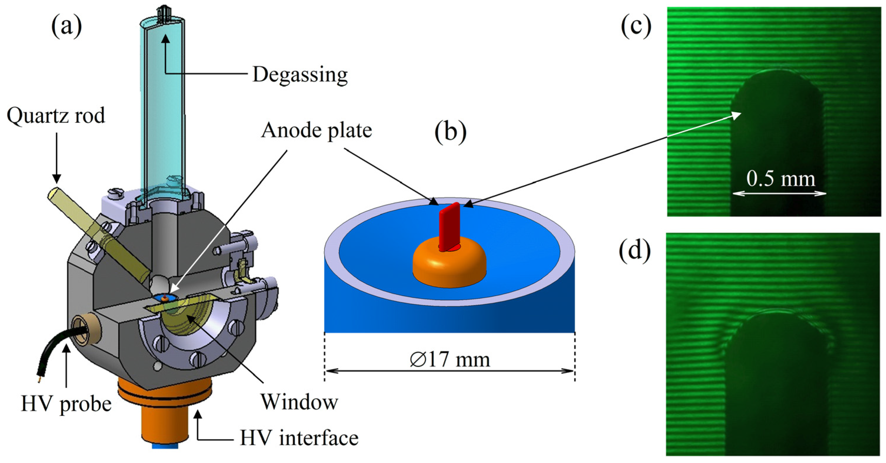
Figure 2.
Block scheme of the interferometric (Mach–Zehnder) setup: P—polarizer; A—analyzer; M1 and M2—mirrors; RB—reference beam; PB—probing beam; ChD—delay chamber; ChM—measurements chamber with the plate anode; BS1 and BS2—beam splitters; PMT—photomultiplier; L1 and L2—objective lenses; FID—high-voltage pulsed source; CP—signal from the capacitive probe.

Figure 3.
Typical waveforms of voltage acquired by the capacitive probe and the photomultiplier detecting the laser pulse.
Figure 3.
Typical waveforms of voltage acquired by the capacitive probe and the photomultiplier detecting the laser pulse.
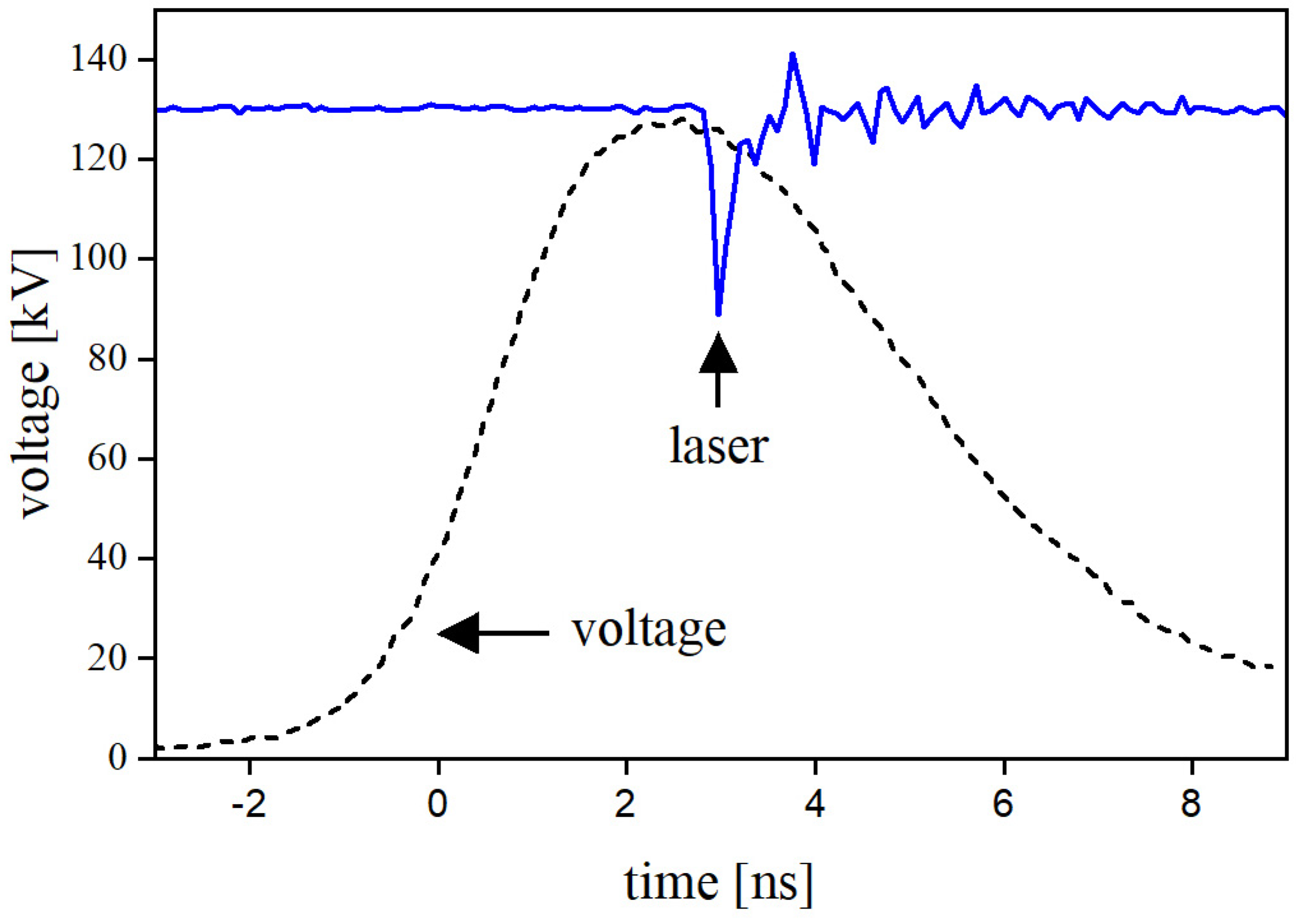
Figure 4.
Orientation of axes with respect to the plate anode (a) and z–component of electric field in the y–z plane calculated at a voltage of 150 kV and corresponding ∆n determined by Equation (1) (b). The position of the electrode apex corresponds to z = 0, and vertical axes of symmetry correspond to x = 0 and y = 0.
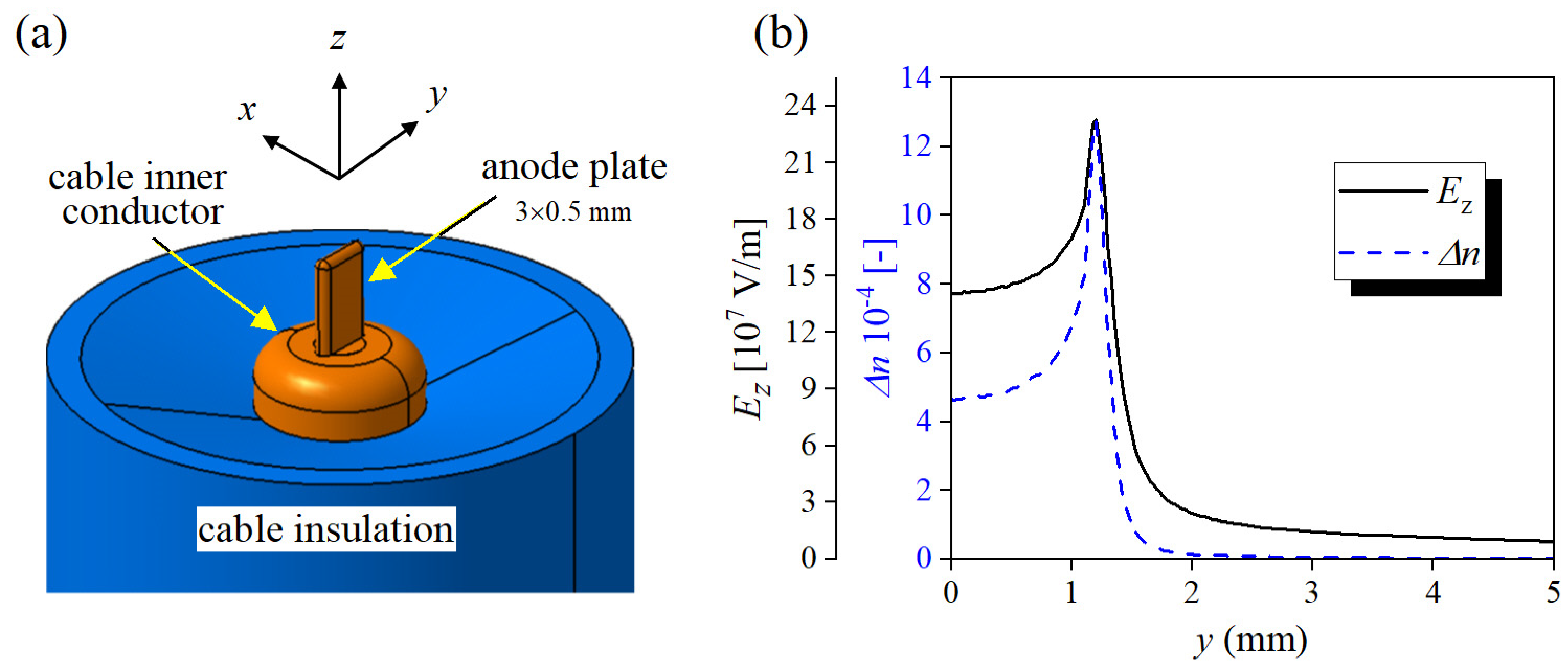
Figure 5.
Estimation of contribution to the total phase shift of the probing beam at a voltage of 150 kV in the areas where the electric field is appreciable. Distribution of electric field around the anode plate in the y–z plane is indicated by the red arrows.
Figure 5.
Estimation of contribution to the total phase shift of the probing beam at a voltage of 150 kV in the areas where the electric field is appreciable. Distribution of electric field around the anode plate in the y–z plane is indicated by the red arrows.
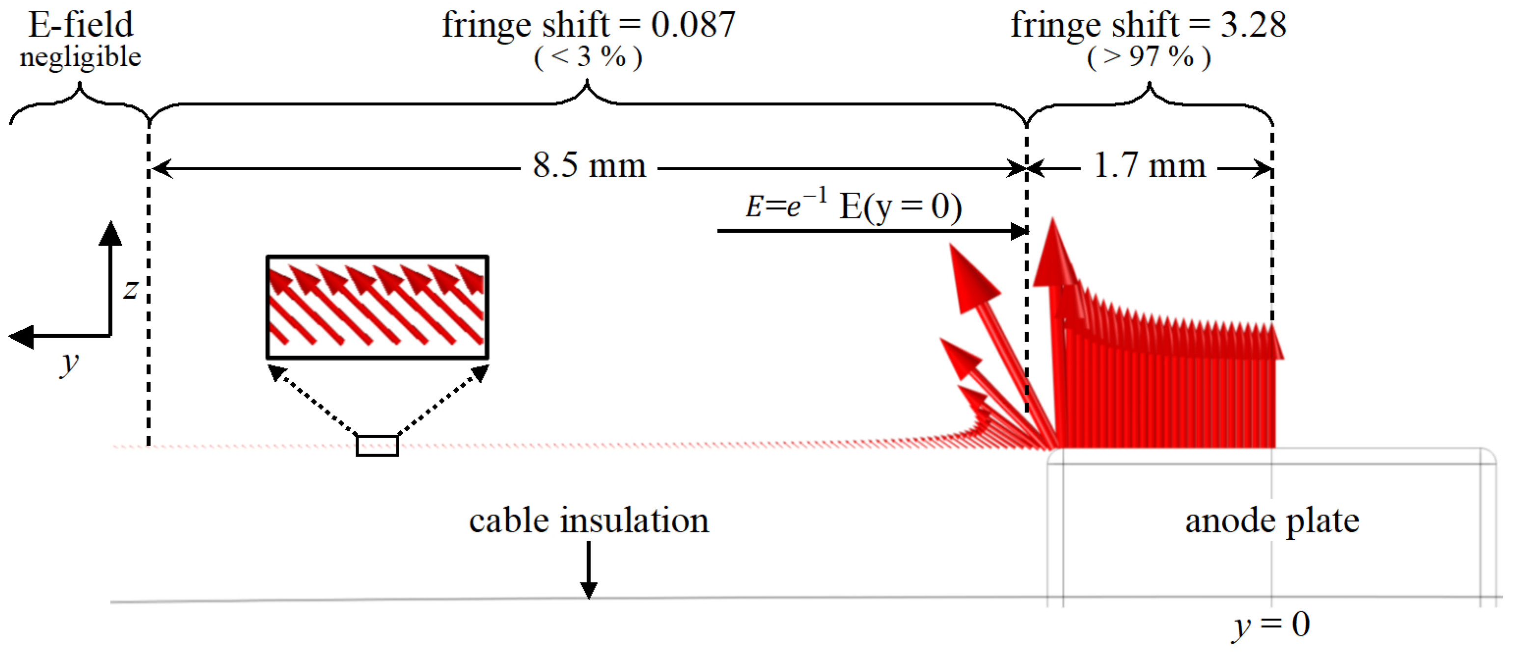
Figure 6.
Spectrum of the voltage pulse generated by the FID.

Figure 7.
Description of fringe pattern in a typical interferogram: fringe deviation at zero field due to optical system distortion (a) and fringe pattern destruction and shift due to electric field (time delay from the voltage pulse onset and voltage are 3 ns/154 kV) (b). The anode plate edge is outlined for better visibility. Vertical laser polarization.

Figure 8.
Examples of (a) single-corner discharge and (b) two-corner discharge. Peak electrode voltage is ~175 kV and time delay from the voltage pulse onset and laser is approximately 3 ns.
Figure 8.
Examples of (a) single-corner discharge and (b) two-corner discharge. Peak electrode voltage is ~175 kV and time delay from the voltage pulse onset and laser is approximately 3 ns.
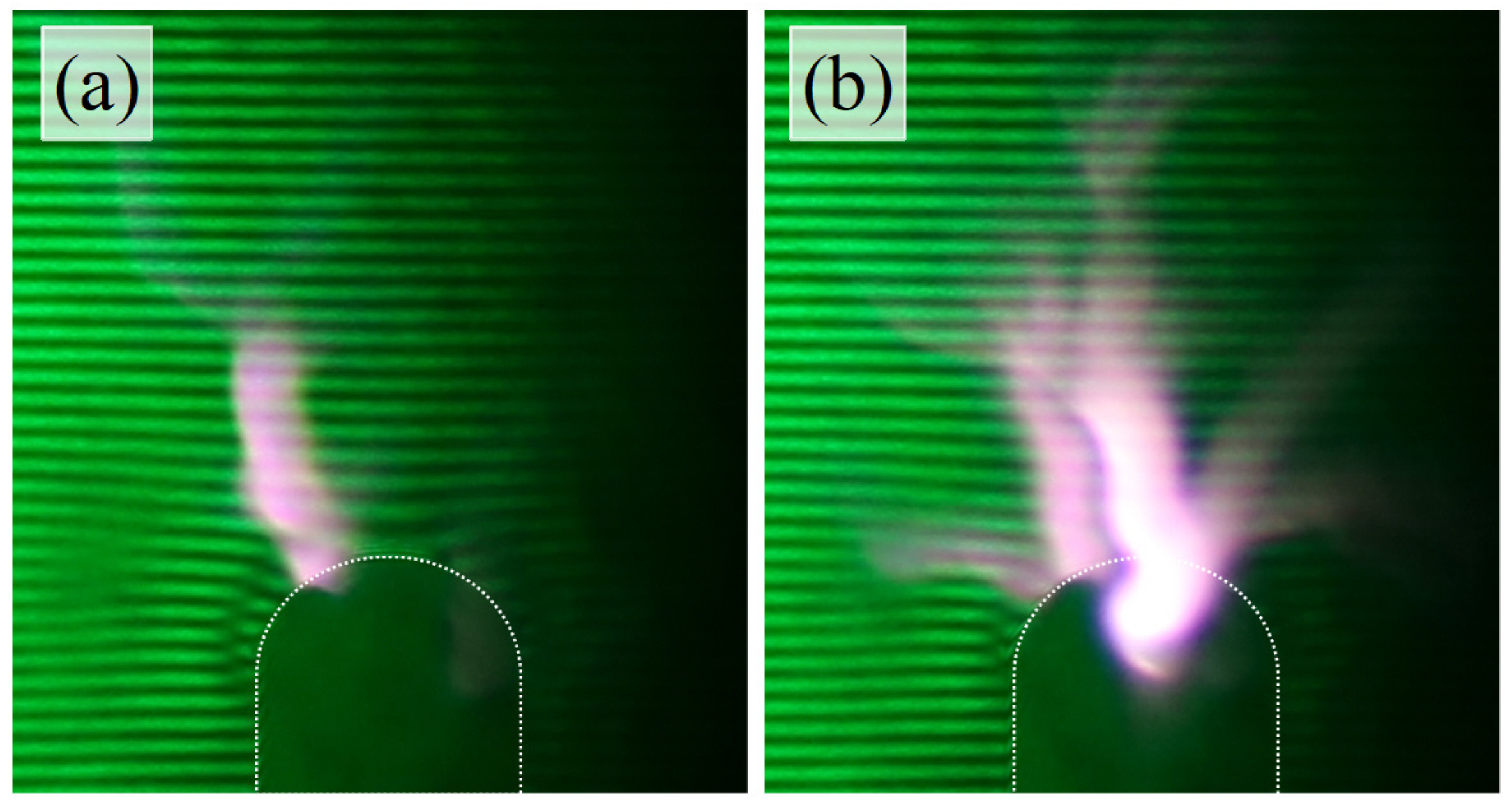
Figure 9.
Morphology of the electrode tip in the central area and edges. Macroscopic views (a–c,g–i) and detail (d–f). Yellow arrows in (a,c,g,i) point to the path on which the discharge was evidently preferentially formed.
Figure 9.
Morphology of the electrode tip in the central area and edges. Macroscopic views (a–c,g–i) and detail (d–f). Yellow arrows in (a,c,g,i) point to the path on which the discharge was evidently preferentially formed.

Figure 10.
Series of interferograms demonstrating fringe distortion at different voltages and laser polarizations. The images do not preserve the original aspect ratio (larger horizontal scale) for better fringe shift visibility. The interferometer is set up such that the fringes always shift in the presence of electric field towards the electrode at the axis of symmetry.
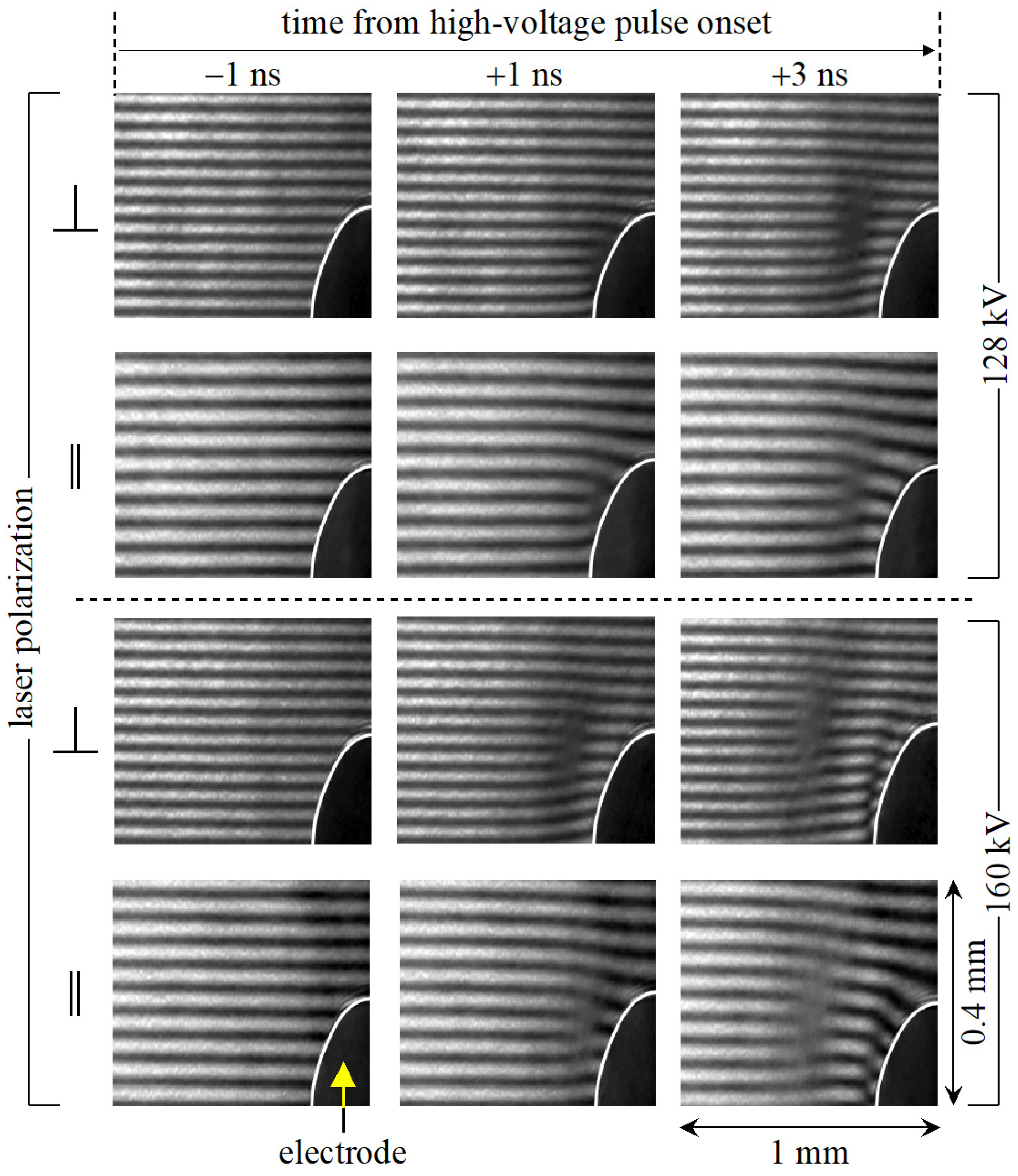
Figure 11.
Time dependence of phase shift in both laser polarizations (a,c) and corresponding reconstructed electric field waveforms together with the voltage waveforms gained from the HV probe (b,d). The voltage amplitude was 128 kV (a,b) and 160 kV (c,d).
Figure 11.
Time dependence of phase shift in both laser polarizations (a,c) and corresponding reconstructed electric field waveforms together with the voltage waveforms gained from the HV probe (b,d). The voltage amplitude was 128 kV (a,b) and 160 kV (c,d).

Figure 12.
Numerical simulations of the z-component of the electric field (full blue line) with the calculated rise in the phase shift (dashed black line) due to the Kerr effect along the path (of the laser beam) perfectly aligned with the y-axis (a), and along the path that slightly leaned in the z-direction causing apparent field distortion (b). The electrode voltage in the simulation is 160 kV.
Disclaimer/Publisher’s Note: The statements, opinions and data contained in all publications are solely those of the individual author(s) and contributor(s) and not of MDPI and/or the editor(s). MDPI and/or the editor(s) disclaim responsibility for any injury to people or property resulting from any ideas, methods, instructions or products referred to in the content. |
© 2024 by the authors. Licensee MDPI, Basel, Switzerland. This article is an open access article distributed under the terms and conditions of the Creative Commons Attribution (CC BY) license (https://creativecommons.org/licenses/by/4.0/).
Share and Cite
MDPI and ACS Style
Hoffer, P.; Prukner, V.; Arora, G.; Mušálek, R.; Šimek, M. Determination of Highly Transient Electric Field in Water Using the Kerr Effect with Picosecond Resolution. Plasma 2024, 7, 316-328. https://doi.org/10.3390/plasma7020018
AMA Style
Hoffer P, Prukner V, Arora G, Mušálek R, Šimek M. Determination of Highly Transient Electric Field in Water Using the Kerr Effect with Picosecond Resolution. Plasma. 2024; 7(2):316-328. https://doi.org/10.3390/plasma7020018
Chicago/Turabian StyleHoffer, Petr, Václav Prukner, Garima Arora, Radek Mušálek, and Milan Šimek. 2024. "Determination of Highly Transient Electric Field in Water Using the Kerr Effect with Picosecond Resolution" Plasma 7, no. 2: 316-328. https://doi.org/10.3390/plasma7020018