Improved Modelling of a Nonlinear Parametrically Excited System with Electromagnetic Excitation

Abstract

In this work, the nonlinear behaviour of a parametrically excited system with electromagnetic excitation is accurately modelled, predicted and experimentally investigated. The equations of motion include both the electromechanical coupling factor and the electromechanical damping. Unlike previous studies where only linear time-varying stiffness due to electromagnetic forces was presented, in this paper the effect of the induced current is studied. As a consequence, nonlinear parameters such as electromechanical damping, cubic stiffness and cubic parametric stiffness have been included in the model. These parameters are also observed experimentally by controlling the direct current (DC) and alternating current (AC) passed through the electromagnets. In fact, the proposed apparatus allows to control both linear and nonlinear stiffnesses and the independent effect of each parameter on the response is presented. In particular the effect of the cubic parametric stiffness on the parametric resonance amplitudes and the influence of cubic stiffness on the frequency bandwidth of the parametric resonance are shown. This model improves the prediction of parametric resonance, frequency bandwidth, and the response amplitude of parametrically excited systems and it may lead to refined design of electromagnetic actuators, filters, amplifiers, vibration energy harvesters, and magnetic bearings.

1. Introduction

Parametrically Excited (PE) systems, where system parameters vary periodically with an independent variable (time) can be found in electrical and mechanical systems [1,2]. Parametric resonance is caused by time-varying system parameters. One of the first documents in observing a PE system was released by Faraday in 1831 [3]. He observed parametric excitation in a vertically oscillating cylinder on the surface of a fluid which had half the frequency of the excitation. Lord Rayleigh in 1883 [4] devised an experiment to show the PE system behaviour. The experiment was based on a taut string attached to a tuning fork. When the tuning fork vibrated vertically the fundamental vibration frequency in string was observed to be half the tuning fork frequency. A playground swing-set is a simple example of parametric excitation in a physical system. The swing is like a pendulum, whose moment of inertia changes with time in a periodic manner. The frequency of this change is called parametric frequency. The user of the swing will squat to increase the swing height without being pushed. If the frequency of the periodic oscillation of the user is equal to twice the frequency of the periodic oscillation from the swing, the amplitude will increase progressively. This large movement happens at Parametric Resonance (PR). PR occur near the drive frequencies of $\frac{2{\omega }_{\mathrm{n}}}{m}$, where ${\omega }_{\mathrm{n}}$ is the system’s natural frequency and m is an integer greater than 1. Due to the high amplitude of responses as a result of parametric resonance, parametrically excited systems have been used to amplify external harmonic signals in electrical engineering applications.

Nonlinear tuning techniques have been exploited to generate parametric resonance in single frequency bandpass filters and vibration energy harvesters [5]. Desired frequency response characteristics are achieved by introducing the linear and cubic nonlinear stiffness. A higher frequency bandwidth and controllable stop-band rejection can be achieved by controlling the nonlinearity in a Nonlinear Parametrically Excited (NPE) system. Rhoads et al. [6] introduced electrostatically driven microelectromechanical systems, which were used to design a bandpass filter. However, in order to overcome the damping force and achieve parametric resonance the alternating current had to be considerably increased, so greater input energy was needed.

Various geometries have been chosen to design NPE oscillators, such as spring mass structures [7], cantilever beams [8], and torsional spring oscillators [9]. The axially driven cantilever beam is extensively used due to its simple geometry, well known analytical model, and ease of fabrication. The axial load on the cantilever beam produces parametric excitation, which results in time-dependent coefficients in the governing differential equation of motion. The stiffness of the beam is influenced by an axial force, and the time-varying axial load generates a parametric excitation [10]. By setting the parametric excitation at different frequencies, amplification [11] or suppression [2] can be observed. The effective nonlinearity in the axially driven cantilever beam due to curvature and inertia is studied in [12]. For a beam, geometric and inertia nonlinearities are a function of the geometry of the beam, material properties, boundary conditions, curvature, and mode shapes. By altering one or a combination of these parameters, the effective nonlinearity of the beam can be changed, achieving the desired bend in the frequency response. These nonlinearities are exploited in the design of PE harvesters [13]. As well as geometry variation, parametric resonance can be obtained using different methods of actuation, such as piezoelectric [14], electrostatic [6], and electromagnetic [15]. Electromagnetic micro-transducers have been used in distinct applications in recent years [16]. A PE cantilever beam with an electromagnetic device was introduced by Chen and Yeh [17,18]. A further study on a Linear Parametrically Excited (LPE) cantilever beam with an electromagnetic system was carried out by Han et al. [19]. In this system, the amplitude and frequency of the time-varying stiffness were accurately controlled by the current flowing through the coil of the electromagnetic device. They showed that, by exciting the cantilever beam with a time-varying force, the nonlinearity induced by the geometric imperfection of the beam and the coupling effects between the excitation mechanism and the beam were effectively avoided [18]. Therefore, they introduced a LPE system where the strong stiffness nonlinearities present in the electromagnetic system were not considered. Several techniques have been introduced in the literature [20] to identify the relationship between the applied electromagnetic force and the resulting displacement in an electromagnetically actuated cantilever beam. Since the elastic force acting on the magnets attached to the cantilever beam is created through magnetic repulsion, the relation between the beam displacement and the resulting elastic restoring force is nonlinear. The nonlinear parameters can be estimated by curve-fitting through data recorded by a force gauge attached to the magnets [20]. A polynomial interpolation through the experimental points provides a mathematical expression; however, this method is limited due to the physical connection of the force gauge.

In this paper, a cantilever beam is investigated. Time-varying stiffness and nonlinear stiffness are applied by an electromagnetic system. The effects of nonlinear damping, time-varying stiffness and nonlinear stiffness are demonstrated independently, which are the main contributions of this paper. A novel approach is presented to calculate the nonlinear electromagnetic forces. The analytical expression obtained for cubic parametric stiffness and cubic stiffness allow us to identify system parameters to increase the amplitude of the response or the frequency bandwidth. The electromechanical coupling factor between the pair of coils and magnets, and the induced current generated by the moving magnets and coils, are included in the model of the NPE system. The induced current generates nonlinear damping, which affects the amplitude of the response. This has been neglected in previous studies, and its importance is highlighted in this paper.

This paper is arranged as follows: the next section introduces the equation of motion describing the NPE system with electromagnets as well as the experimental set-up. The mathematical explanation of the electromechanical system is presented in Section 2.2. The effect of direct and alternating current on changing the damping, resonance frequency, and stiffness is described in Section 2.3, which informs the mathematical model of the NPE system as explained in Section 2. A parametric study is carried out and the behavior of the system response is illustrated in Section 3. The effect of damping, time-varying stiffness, and nonlinearities on the response of the NPE system are carried out experimentally and analytically in Section 3.2 and Section 3.3.

2. Theory

In this study, SDOF equation of motion of a NPE system is considered:

$$\begin{array}{c}\ddot{z}+2{\omega }_{\mathrm{n}}{\zeta }_{\mathrm{m}}\dot{z}+2{\omega }_{\mathrm{n}}{\zeta }_{\mathrm{es},\mathrm{app}}{z}^2\dot{z}+{\omega }_{\mathrm{n}}^2{\delta }_{\mathrm{es},\mathrm{app}}{z}^2\dot{z}+{\omega }_{\mathrm{n}}^2{\gamma }_{\mathrm{es},\mathrm{app}}{z}^4\dot{z}+\\ {\omega }_{\mathrm{n}}^2\left(1+\delta cos(\mathsf{\Omega }t)\right)z+{\omega }_{\mathrm{n}}^2\left(\alpha +\gamma cos(\mathsf{\Omega }t)\right)z^3=0,\end{array}$$

(1)

where the nonlinear damping, linear time-varying forces, and nonlinear forces applied from the electromagnets. The system parameters are derived analytically in Section 2.3. In Equation (2), z is the displacement of the mass, ${\zeta }_{\mathrm{m}}$ is the linear damping factor, ${\zeta }_{\mathrm{es},\mathrm{app}}$, ${\delta }_{\mathrm{es},\mathrm{app}}$ and ${\gamma }_{\mathrm{es},\mathrm{app}}$ are the nonlinear damping coefficients, $\mathsf{\Omega }$ is the parametric frequency, ${\omega }_{\mathrm{n}}$ is the natural frequency, $\delta$ is the normalized time-varying stiffness, $\alpha$ is the cubic stiffness, and $\gamma$ is the cubic parametric stiffness.

Equation (1) is normalized by time scaling $\tau =\mathsf{\Omega }t$ and expressed with derivatives with respect to $\tau$ instead of t. Normalization in this way results in following equation of motion:

$$\begin{array}{c}{z}^{″}+\frac{2\epsilon {\zeta }_{\mathrm{m}}{\omega }_{\mathrm{n}}}{\mathsf{\Omega }}{z}^{\prime }+\frac{2\epsilon {\zeta }_{\mathrm{es},\mathrm{app}}{\omega }_{\mathrm{n}}}{\mathsf{\Omega }}{z}^2{z}^{\prime }+\frac{{\omega }_{\mathrm{n}}^2}{\mathsf{\Omega }}\left(\epsilon {\delta }_{\mathrm{es},\mathrm{app}}\right)z^2{z}^{\prime }+\frac{{\omega }_{\mathrm{n}}^2}{\mathsf{\Omega }}\left(\epsilon {\gamma }_{\mathrm{es},\mathrm{app}}\right)z^4{z}^{\prime }+\\ \frac{{\omega }_{\mathrm{n}}^2}{{\mathsf{\Omega }}^2}\left(1+\epsilon \delta cos\left(\tau \right)\right)z+\frac{{\omega }_{\mathrm{n}}^2}{{\mathsf{\Omega }}^2}\left(\epsilon \alpha +\epsilon \gamma cos\left(\tau \right)\right)z^3=0.\end{array}$$

(2)

The prime ${(.)}^{\prime }$ is used to present a quantity differentiated with respect to $\tau$. $\epsilon$ times the system parameter denotes terms that have a low order of magnitude.

The method of averaging [21] is an approximation method, used here to find the solutions of Equation (1). The parametric frequency $\mathsf{\Omega }$ is varied around a reference frequency ${\mathsf{\Omega }}_0$ thus

$$\mathsf{\Omega }={\mathsf{\Omega }}_0\left(1-\epsilon \mathsf{\Delta }\right),$$

(3)

where $\mathsf{\Delta }$ is the detuning parameter. The solution of Equation (2) for $\epsilon =0$ is a linear combination of $cos(\tau )$ and $sin(\tau )$:

$$z\left(\tau \right)=acos\left(\kappa \tau +\phi \right),$$

(4)

where a and $\phi$ are the constant amplitude and phase respectively, which can be determined from initial conditions. The frequency ratio

$$\kappa =\frac{{\omega }_{\mathrm{n}}}{{\mathsf{\Omega }}_0}$$

(5)

is used here for simplification. When $\epsilon \ne 0$, based on the method of Lagrange [21], we assume that the solution can still be written in the format of Equation (4), with time-varying amplitude a and phase $\phi$. Consequently, the solution of Equation (2) is

$$z\left(\tau \right)=a\left(\tau \right)cos\left(\mathsf{\Phi }\left(\tau \right)\right),$$

(6)

where $\mathsf{\Phi }\left(\tau \right)=\kappa \tau +\phi \left(\tau \right)$, and

$$z^{\prime }\left(\tau \right)=a^{\prime }\left(\tau \right)cos\left(\mathsf{\Phi }\left(\tau \right)\right)-a\left(\tau \right)(\kappa +{\phi }^{\prime }\left(\tau \right))sin\left(\mathsf{\Phi }\left(\tau \right)\right).$$

(7)

Substituting Equations (6) and (7) into Equation (2) results in an equation which can be solved for $a^{\prime }\left(\tau \right)$ and ${\phi }^{\prime }\left(\tau \right)$. $a^{\prime }\left(\tau \right)$ and ${\phi }^{\prime }\left(\tau \right)$ are then averaged over one period $T=\frac{2\pi }{\mathsf{\Omega }}$ under the assumption that $a\left(\tau \right)$ and $\phi \left(\tau \right)$ change slowly. The resulting averaged equation can be integrated with respect to $\tau$ to find $a\left(\tau \right)$ and $\phi \left(\tau \right)$ for a given $\kappa$ and reference frequency ${\mathsf{\Omega }}_0$. The steady-state behavior of the system can be recovered from the set of $a^{\prime }\left(\tau \right)$ and ${\phi }^{\prime }\left(\tau \right)$ by setting $(a^{\prime },{\phi }^{\prime })=(0,0)$ and solving for steady-state values of a and $\phi$. Thus, the resulting solution is an approximation of the original solution. For non-zero $\epsilon$, the solutions can be found from:

$$a^{\prime }(\tau )=\frac{\epsilon \gamma a^3}{16}sin\left(2\phi \right)-\frac{\epsilon {\zeta }_{\mathrm{m}}{\omega }_{\mathrm{n}}a}{\mathsf{\Omega }}+\frac{\epsilon \delta a}{8}sin\left(2\phi \right)-\frac{\epsilon {\zeta }_{\mathrm{es},\mathrm{app}}{\omega }_{\mathrm{n}}{a}^3}{4\mathsf{\Omega }}-\frac{\epsilon {\gamma }_{\mathrm{es},\mathrm{app}}{a}^4\mathsf{\Omega }}{256}+\mathcal{O}({\epsilon }^2),$$

(8)

$$\begin{array}{c}{\phi }^{\prime }(\tau )=\frac{\epsilon \mathsf{\Delta }}{2}+\frac{\epsilon \gamma a^2}{8}cos\left(2\phi \right)+\frac{3\epsilon \alpha a^2}{16}+\frac{\epsilon \delta }{8}cos\left(2\phi \right)-\frac{\epsilon {\delta }_{\mathrm{es},\mathrm{app}}{a}^2\mathsf{\Omega }}{32}sin(2\phi )-\\ \frac{5\epsilon {\gamma }_{\mathrm{es},\mathrm{app}}{a}^4\mathsf{\Omega }}{256}sin(2\phi )+\mathcal{O}({\epsilon }^2).\end{array}$$

(9)

2.1. Apparatus

The electromagnetic system in Figure 1a is used to produce the time-varying stiffness desired in the experimental model. The electromagnetic set-up was adopted and modified based on the work of F. Dohnal [2,22]. In this set-up controlling direct and alternating input current carried by the coils gives the possibility of changing system’s parameters such as the damping coefficient, linear and nonlinear stiffness. The cantilever beam is at equilibrium when the two coils carry the same direct current, and the magnets are positioned at the same distance h from the center of coils. The mutual electromagnetic forces acting between the coils and magnets cause the electromagnetic device to act as a nonlinear spring. If the magnets and coils are repulsive, the attached beam returns to its equilibrium position when the beam is perturbed. In this case, the stiffness produced by the electromagnetic device is positive. In this paper, only repulsive forces and consequently positive stiffness are considered. In Figure 1a position of the electromagnets is chosen to approximate the system as a SDOF model. In this position, the first and second modes are apart to maintain the SDOF model approximation. The first and the second natural frequencies are mentioned in

Table 1. Mechanical properties and dimensions.

Property	Value	Units
Radius of the Neodymium (N42) disc magnets	$0.015$	$\mathrm{m}$
Residual magnetic flux density of the permanent magnet ($B_{\mathrm{r}}$)	$1.1$	T
Permeability (${\mu }_0$)	$4\pi {10}^{-7}$	$\mathrm{N}{\mathrm{A}}^{-2}$
Inner radius of the coil type L71-3,30 from Mundorf ($r_1$)	$0.0085$	$\mathrm{m}$
Outer radius of the coil ($r_2$)	$0.0225$	$\mathrm{m}$
Mean radius of the coil ($r_{\mathrm{c}}$)	$0.0135$	$\mathrm{m}$
Number of turns of in coil (N)	485	-
Length of wire in one rotation ($l_{\mathrm{w}}$)	0.078	$\mathrm{m}$
Diameter of the coil ($D_{\mathrm{w}}$)	0.00071	$\mathrm{m}$
Height of the coil with shield ($h_{\mathrm{coil}}$)	0.02	$\mathrm{m}$
Coordinate for coil ($z_1$)	0.007	$\mathrm{m}$
Coordinate for coil ($z_2$)	−0.007	$\mathrm{m}$
Measured electrical resistance of the coil and extra wiring ($R_{\mathrm{coil}}$)	1.91	Ohm
Resistor (R)	0.1	Ohm
Width of the beam ($b_{\mathrm{b}}$)	$0.01$	$\mathrm{m}$
Thickness of the beam ($t_{\mathrm{b}}$)	$0.002$	$\mathrm{m}$
Total physical mass (the effective mass of the beam and magnets) ($m_{\mathrm{t}}$)	$0.104$	$\mathrm{kg}$
Static stiffness of the beam with magnets and coils when $I_{\mathrm{c}}=0$ ($k_{\mathrm{b}}$)	32.84	${\mathrm{Nm}}^{-1}$
Measured first natural frequency of the beam with magnets and coils when $I_{\mathrm{c}}=0$ (${\omega }_{\mathrm{n}},\exp$)	17.76	$\mathrm{rad}{\mathrm{s}}^{-1}$
Measured second natural frequency of the beam with magnets and coils when $I_{\mathrm{c}}=0$	202	$\mathrm{rad}{\mathrm{s}}^{-1}$
Mechanical damping coefficient of the beam with magnets and coils when $I_{\mathrm{c}}=0$ ($c_{\mathrm{m}}$)	0.011	${\mathrm{Nsm}}^{-1}$

. The ratio between the second mode and the first mode is considered to be greater than 4 in order to reduce the effect of higher modes on the response [23]. The influence of higher modes on the response amplitude when the current is generated in the coils have not been considered in this paper.

To generate the electromagnetic force, two electromagnetic configurations are considered, coils connected in series and in parallel with opposing connection. Connecting the coils in series increases the internal resistance, which reduces the electrical damping. Reducing the total damping lowers the transition curves and changes the stability threshold of the PE system [24]. However, the parallel opposing connection has an increased electrical damping due to circulating current. To reduce electrical damping, the series configuration is used in this study. The schematics of the experimental set-up and the parameters for the electromagnetic system and the beam are provided in Figure 1b and Table 1, respectively.

2.2. Mathematical Model

The experimental set-up is modelled mathematically as a mechanical system coupled to an electric circuit. Figure 2 shows the coupled mechanical and electromagnetic systems, where the coils in the electromagnetic system are in the series opposing connection. The coils are identical, and each coil is modelled with a resistance and an inductance.

The equations governing the motion of the mechanical is:

$$m_{\mathrm{t}}\ddot{z}+c_{\mathrm{m}}\dot{z}+k_{\mathrm{b}}z+F_{\mathrm{e}}(z)+F_{\mathrm{emf}}(z)=0,$$

(10)

where the overdot represents a derivative with respect to time, t. The variable z represents the displacement of the system mass $m_{\mathrm{t}}$ (the effective mass of the beam with the attached magnets), the linear viscous damping coefficient $c_{\mathrm{m}}$ is equivalent to the linear viscous damping coefficient of the beam, $k_{\mathrm{b}}$ is chosen equal to the static stiffness of the cantilever beam, and $F_{\mathrm{e}}(z)$ is the electromagnetic force generated as a result of coils carrying current (explained in detail in the next section). $F_{\mathrm{emf}}(z)$ is the electromagnetic force induced by the interaction of oscillating magnet and coils. The voltage equation of the electric circuit is:

$$V=2L_{\mathrm{coil}}{\dot{I}}_{\mathrm{c}}+\left(R+2R_{\mathrm{coil}}\right)I_{\mathrm{c}}+V_{\mathrm{emf}},$$

(11)

$L_{\mathrm{coil}}$ and $R_{\mathrm{coil}}$ are the inductance and the internal resistance of the coil, respectively. The inductance of the coil $L_{\mathrm{coil}}$ is estimated based on [25] as $0.64$ mH. The maximum reactance due to inductance for the maximum frequency used in this study is $15$ Hz and hence reactance $Z_{\mathrm{coil}}=2\pi f(2\times 0.64\times {10}^{-3})=0.12$ Ohm, where f is the frequency. This reactance is less than 4 percent of the total resistance of the coil and hence $L_{\mathrm{coil}}$ is considered negligible. In Equation (11) $I_{\mathrm{c}}$ is the current generated by the power supply

$$I_{\mathrm{c}}=I_{\mathrm{DC}}+I_{\mathrm{AC}}cos(\mathsf{\Omega }t),$$

(12)

where $I_{\mathrm{DC}}$ is the direct current and $\mathsf{\Omega }$ is the frequency of the alternating current, $I_{\mathrm{AC}}$. In Equation (11) $V_{\mathrm{emf}}$ is the induced voltage from the moving magnets along the axis of the coils, which cause induced current $i_{\mathrm{es}}$ to flow in coils. Hence, the total current flow in coils is

$$I=I_{\mathrm{c}}+i_{\mathrm{es}}.$$

(13)

2.3. Parameter Identification

The parameters of Equation (10) are identified in this section. $F_{\mathrm{e}}(z)$ and $F_{\mathrm{emf}}(z)$ are presented analytically based on system parameters. Magnetic field $B_{\mathrm{z}}$ generated by the two pairs of coils can be obtained from the Biot-Savart law,

$$B_{\mathrm{z}}(z)=-\frac{{\mu }_0{r}_{\mathrm{c}}^{2}IN}{2{({(h+z)}^2+r_{\mathrm{c}}^2)}^{\frac{3}{2}}}-\frac{{\mu }_0{r}_{\mathrm{c}}^{2}IN}{2{({(z-h)}^2+r_{\mathrm{c}}^2)}^{\frac{3}{2}}},$$

(14)

h is the distance between the center of coil and the equilibrium position, and other parameters are defined in Table 1. Equation (14) is differentiated to find the electromagnetic force $F_{\mathrm{e}}$. Using the Taylor expansion about $z=0$, the force applied to the cantilever beam can be expressed as

$$F_{\mathrm{e}}(z)=H_{1}Iz+H_{2}I{z}^3+\mathcal{O}(z^5),$$

(15)

where $H_1$ and $H_2$ are

$$H_1=\frac{3}{2}\mu {\mu }_0{r}_c^{2}N\left(\frac{-2}{{\left(h^2+{r_{\mathrm{c}}}^2\right)}^{\frac{5}{2}}}+\frac{10h^2}{{\left(h^2+{r_{\mathrm{c}}}^2\right)}^{\frac{7}{2}}}\right),$$

(16)

$$H_2=\frac{3}{2}\mu {\mu }_0{r}_c^{2}N\left(\frac{5}{{\left(r_{\mathrm{c}}^2+h^2\right)}^{\frac{7}{2}}}-\frac{70h^2}{{\left(r_{\mathrm{c}}^2+h^2\right)}^{\frac{9}{2}}}+\frac{105h^4}{{\left(r_{\mathrm{c}}^2+h^2\right)}^{\frac{11}{2}}}\right).$$

(17)

The difference between the exact $F_e$ and the third-order polynomial approximation increases with absolute z. For the configuration $h=0.035$ m, $\left|z\right|\le 0.015$ m, which corresponds to a relative error of $8.3\%$. A higher-order approximation using a fifth-order polynomial expansion reduces the error to $0.42\%$. These percentage errors decrease greatly with decreasing absolute z. The former error is acceptable for this study. When h is increased to $h=0.035$ m, then $\left|z\right|\le 0.025$, and the relative error for the third-order approximation increases to $22\%$, and for the fifth-order approximation increases to $10\%$. While this error is greater than the error for the case with lower z, the approximation still demonstrates agreement with the experimental results which is shown in Section 3.1, particularly when z is far from maximum.

Based on Lenz’s law, the force $F_{\mathrm{emf}}(z)$ in Equation (10) is proportional to the induced current in coils $i_{\mathrm{es}}$,

$$F_{\mathrm{emf}}=k_{\mathrm{t}}(z)i_{\mathrm{es}},$$

(18)

where $k_{\mathrm{t}}(z)$ is electromechanical coupling factor. Analytical expression of $k_{\mathrm{t}}(z)$ is found from calculating the magnetic field based on [26]. The magnetic field generated by the moving magnet can be approximated as [26]

$$\mathbf{B}=\frac{V_{\mathrm{m}}{B}_{\mathrm{r}}}{4\pi }\left(\frac{3r(h-z){\widehat{\mathbf{e}}}_{\mathbf{r}}-\left(r^2-2(h-z)\right){\widehat{\mathbf{e}}}_{\mathbf{z}}}{{\left(r^2+{(h-z)}^2\right)}^{\frac{5}{2}}}\right),$$

(19)

where $V_{\mathrm{m}}$ is the volume of the magnet, $B_{\mathrm{r}}$ is the residual magnetic flux density, ${\widehat{\mathbf{e}}}_{\mathbf{r}}$ is a unit vector pointing in the positive r direction and ${\widehat{\mathbf{e}}}_{\mathbf{z}}$ is a unit vector pointing in the positive z direction (see Figure 3). When the magnet is moved along the axis of the coil, an electric potential across the coils is generated

$$V_{\mathrm{emf}}=\frac{\mathrm{d}}{\mathrm{d}t}\underset{A}{\int }\mathbf{B}\mathrm{d}A=k_{\mathrm{t}}(z)\dot{z},$$

(20)

where A indicates the area enclosed by the wire loop. The quantity $k_{\mathrm{t}}$ is the nonlinear electromechanical coupling, which for two coils in series and a magnet is

$$\begin{array}{c}\hfill k_{\mathrm{t}}(z)=\frac{3\varsigma V_{\mathrm{m}}{B}_{\mathrm{r}}}{2(r_2-r_1)(z_2-z_1)}\left(\sum _{n,m=1}^2{(-1)}^{n+m}{z}_{\mathrm{nm}}\right),\end{array}$$

(21a)

$$z_{\mathrm{nm}}=ln(r_{\mathrm{n}}+z_{\mathrm{nm}}^{\prime })-\frac{r_{\mathrm{n}}}{z_{\mathrm{nm}}^{\prime }}-ln(r_{\mathrm{n}}+z_{\mathrm{nm}}^{″})+\frac{r_{\mathrm{n}}}{z_{\mathrm{nm}}^{″}},$$

(21b)

$$z_{\mathrm{nm}}^{\prime }=\sqrt{r_{\mathrm{n}}^2+{\left(z_{\mathrm{m}}-(z+h)\right)}^2},$$

(21c)

$$z_{\mathrm{nm}}^{\prime \prime }=\sqrt{r_{\mathrm{n}}^2+{\left(z_{\mathrm{m}}-(-z+h)\right)}^2},$$

(21d)

where $D_{\mathrm{w}}$ is the coil diameter, $l_{\mathrm{w}}$ is the length of the wire in one rotation, N is the number of turns in each coil, $h_{\mathrm{coil}}$ is the height of the coil, and $r_1$ and $r_2$ are the inner and outer radius of the coil respectively. Please note that assumptions for the nonlinear coupling coefficient may not be valid for all coil configurations, and careful consideration is needed when the electromagnetic system geometry is varied.

The change of electromechanical coupling with respect to z is considered linear $k_t(z)=k_{\mathrm{t},\mathrm{app}}z+\mathcal{O}(z^2)$, where $k_{\mathrm{t},\mathrm{app}}={\left.\frac{\partial k_{\mathrm{t}}(z)}{\partial z}\right|}_{z=0}$. The first term of the $k_{\mathrm{t}}$ expansion ($k_{\mathrm{t},\mathrm{app}}z$) has a unity order of magnitude. This order of magnitude is found by first using Equation (21) to determine ${\left.\frac{\partial k_{\mathrm{t}}(z)}{\partial z}\right|}_{z=0}$, then the product ${\left.\frac{\partial k_{\mathrm{t}}(z)}{\partial z}\right|}_{z=0}z$ is maximized to determine the order of magnitude for z values mentioned in this paper. The second term of the $k_{\mathrm{t}}$ expansion, $({\partial }^2{k}_{\mathrm{t}}/\partial z^2)z^2/2$, has an order of magnitude of ${10}^{-10}$. We conclude that the higher order terms do not significantly affect the $k_{\mathrm{t}}$ approximation for the z values considered in this study.

By considering the approximated electromechanical coupling factor the approximated induced current obtained from Equation (20) is

$$i_{\mathrm{es},\mathrm{app}}=\frac{k_{\mathrm{t},\mathrm{app}}}{2R_{\mathrm{coil}}+R}\dot{z}.$$

(22)

Equation (1) is found by normalizing Equation (10) by $m_{\mathrm{t}}$. In Equation (1) the mechanical damping ratio ${\zeta }_{\mathrm{m}}=\frac{c_{\mathrm{m}}}{2m_{\mathrm{t}}{\omega }_{\mathrm{n}}}$, and ${\zeta }_{\mathrm{es},\mathrm{app}}$ is the electrical damping applied from the electromagnetic system. The dissipative feedback force due to the electromagnetic system can be calculated from substituting Equation (20) into Equation (18). The electrical damping ratio is

$${\zeta }_{\mathrm{es},\mathrm{app}}=\frac{k_{\mathrm{t},\mathrm{app}}^2}{2m_{\mathrm{t}}{\omega }_{\mathrm{n}}\left(2R_{\mathrm{coil}}+R\right)},$$

(23)

where first natural frequency of the cantilever beam with the electromagnetic system ${\omega }_{\mathrm{n}}$ is estimated using the Rayleigh Energy Method. The nonlinear parameters ${\delta }_{\mathrm{es},\mathrm{app}}$ and ${\gamma }_{\mathrm{es},\mathrm{app}}$ are equal to

$${\delta }_{\mathrm{es},\mathrm{app}}=\frac{H_1{i}_{\mathrm{es},\mathrm{app}}}{k_1},$$

(24)

$${\gamma }_{\mathrm{es},\mathrm{app}}=\frac{H_2{i}_{\mathrm{es},\mathrm{app}}}{k_1}.$$

(25)

In Equation (1), normalized parametric stiffness $\delta$, normalized cubic stiffness $\alpha$, and normalized cubic parametric stiffness $\gamma$ are included from electromagnetic forces. The nonlinear terms ${\delta }_{\mathrm{es},\mathrm{app}}$ and ${\gamma }_{\mathrm{es},\mathrm{app}}$ are determined from the effect of induced current. The normalized time-varying stiffness $\delta$ is equal to

$$\delta =\frac{H_1{I}_{\mathrm{AC}}}{k_1},$$

(26)

where $k_1=k_{\mathrm{b}}+I_{\mathrm{DC}}{H}_1$ is the total linear stiffness. The normalised cubic stiffness $\alpha$ is

$$\alpha =\frac{H_2{I}_{\mathrm{DC}}}{k_1}.$$

(27)

The cubic stiffness is strongly affected by the direct current and the parameters of the electromagnetic system, such the distance between the coils, the number of turns in each coil, and the mean radius of the coil. The normalized cubic parametric stiffness is

$$\gamma =\frac{H_2{I}_{\mathrm{AC}}}{k_1}.$$

(28)

For simplicity, expressions involving the quantities $\delta$, $\alpha$ and $\gamma$ will not explicitly state their dependency on current.

3. Free Response of the NPE System

The free response of the NPE system is examined to study the stability and amplitude of the periodic solutions, which depend on the time-varying stiffness and the nonlinear damping and stiffness. If the time-varying stiffness exceeds the stability threshold, the amplitude of the response increases. By reducing the damping, the stability threshold can be reduced. The stability threshold at the parametric resonance can be found from Equations (8) and (9) when nonlinear terms are zero, or by solving Equation (2) using the harmonic balance method [27]. The stability threshold is found to be ${\delta }_{\mathrm{th}}=4{\zeta }_{\mathrm{m}}$. The transition curve for a LPE system is plotted from the analytical calculation in Figure 4a.

Figure 4b shows the amplitude-frequency plot for the cantilever beam excited with linear time-varying and nonlinear forces from the electromagnetic system. The curve describes the cantilever beam displacement a as a function of parametric frequency $\mathsf{\Omega }$ normalized by the linear natural frequency ${\omega }_{\mathrm{n}}$. There are several distinct characteristics for the amplitude-frequency curves of the NPE system (Figure 4b) when compared to the equivalent linear system. Firstly, the response peak bends over to the right, which is the characteristic of nonlinear behavior with restoring forces of the hardening type. Also, for certain values of parametric frequency $\mathsf{\Omega }$, there are multiple solutions.

3.1. Experimental Results

The experimental apparatus and system parameters are presented in Figure 1b and Table 1, with initial displacement $z(0)=z_0=0.01$ m and velocity $\dot{z}(0)=0$. A relay switch, switch 2 in Figure 1b, is used to hold the cantilever beam tip 0.01 m away from the equilibrium position. The relay switch releases the cantilever beam when triggered, and starts the current flow in the coils at the same time.

The system parameters are chosen to express the effect of parametric excitation and stiffness nonlinearity. The direct current for the test in Figure 4b is $I_{\mathrm{DC}}=0.48$ A, and the input alternating current $I_{\mathrm{AC}}=0.06$ A. This direct current is selected to generate a strong cubic stiffness. The alternating current is chosen large enough to generate time-varying stiffness $\delta$, higher than the stability threshold. The induced current is measured while the beam is moving. The linear natural frequency ${\omega }_{\mathrm{n}}=37.11\mathrm{rad}{\mathrm{s}}^{-1}$, and the damping ratio ${\zeta }_{\mathrm{m}}=0.001$, are measured when $I_{\mathrm{c}}=0.48$ A. The system parameters are calculated using Equations (23) to (28) as $\delta =0.093$, $\alpha =1055.86{\mathrm{m}}^{-2}$, $\gamma =131.98{\mathrm{m}}^{-2}$, ${\delta }_{\mathrm{es},\mathrm{app}}=28.82$, and ${\gamma }_{\mathrm{es},\mathrm{app}}=40897.67$.

Point A in Figure 4b is a periodic response. Displacement of the beam (Figure 5a) is found by measuring the velocity with a vibrometer. The velocity signal is filtered with a high-pass filter with a cutoff frequency of $0.1$ Hz. The beam displacement is found by integrating the velocity numerically. Total current in the coils, $I=I_{\mathrm{c}}+i_{\mathrm{es}}$, is plotted in Figure 5b. Frequencies $\mathsf{\Omega }$, $\frac{\mathsf{\Omega }}{2}$, and $\frac{3\mathsf{\Omega }}{2}$ can be seen in the power spectrum density (PSD) plot of the displacement signal (Figure 5c. The PSD plot of the displacement and current signals show that parametric resonance has influenced displacement, so the peak at $\frac{\mathsf{\Omega }}{2}$ has appeared (Figure 5c,d). Direct excitation at $\mathsf{\Omega }$ arises from the misalignment of the magnets; although the set-up was designed to reduce the effect of direct excitation on the response. The PSD plot of the current shows a peak at parametric frequency $\mathsf{\Omega }$ (Figure 5d). The phase portrait plot in Figure 5e shows that point A corresponds to a periodic solution. The Poincaré map in Figure 5f shows two points, indicating two frequencies in the solution that have a ratio of one half. These two points show the displacement and velocity signals contain frequencies of $\frac{\mathsf{\Omega }}{2}$ and $\mathsf{\Omega }$.

After point A in Figure 4b, the amplitude of the response increases smoothly until it jumps to the lower stable branch (trivial solution $a=0$), and stays at rest. During sweep down the amplitude of the response is approximately zero until this solution becomes unstable, at which point it jumps to the higher branch. The frequency at which the jump of free responses of a nonlinear parametrically system occurs depends on the time-varying stiffness and damping as well as the nonlinearities. This experimental approach holds for a single set of initial conditions. As such, it is not appropriate for mapping all possible responses, and so it cannot be used to determine the basins of attraction for each branch.

3.2. Effects of Cubic Parametric Stiffness and Nonlinear Damping

Previous theoretical studies show that, when the time-varying stiffness $\delta$ is greater than instability threshold, the amplitude of the response increases [24]. However, the effect of cubic parametric stiffness on the amplitude of the response has not been studied analytically and experimentally. The analytical amplitude-frequency plot for a NPE system with and without cubic parametric stiffness is presented in Figure 6a. The amplitude of the response is higher for the NPE system with positive cubic parametric stiffness.

Experimental results are shown in Figure 6a. Equations (26) and (28) show that time-varying stiffness $\delta$ and cubic parametric stiffness $\gamma$ are controlled by current $I_{\mathrm{AC}}$ simultaneously, and that when $I_{\mathrm{AC}}\ne 0$, $\gamma \ne 0$ and $\delta \ne 0$. Due to these relations, experimental results for $\delta \ne 0$ and $\gamma =0$ cannot be achieved. For the experimental test, $\delta$ and $\gamma$ are calculated when $I_{\mathrm{DC}}=0.5$ A, and $I_{\mathrm{AC}}=0.2$ A. In Figure 6a a better match between the experimental and analytical results is achieved when non-zero cubic parametric stiffness $\gamma$ is included in the model. Results obtained from several experiments determine that the cubic parametric stiffness is negligible when the altering current is very small or the coils are very close to each other.

Figure 6b shows amplitude-frequency relations for NPE systems with and without nonlinear damping coefficients. The analytical results in this figure show that the response amplitude is reduced for a NPE system with nonlinear damping, and more accurately describes experimental observations. Since the nonlinear damping coefficients are function of induced current, it is not possible to remove this effect experimentally and show the results without the nonlinear damping coefficients.

3.3. The Effects of Cubic Stiffness

The cubic stiffness $\alpha$ present in the NPE system reduces the amplitude of the response relative to the amplitude of the response of the equivalent LPE system at parametric resonance. At different positions between the coils and magnets, a strong cubic stiffness can reduce the jump-down frequencies and the amplitudes of displacement at these frequencies. The cubic stiffness generated by the electromagnetic system increases when the direct current in the coils increases. Also, from the physical derivation, Equation (27), the cubic stiffness $\alpha$ is a function of coil distance h, the radius of the coil, and the number of turns in the coil. To investigate the changes in the cubic stiffness, h is altered between experiments. The maximum ratio between $\alpha$ and $\delta$ can be seen in Figure 7 for a given current.

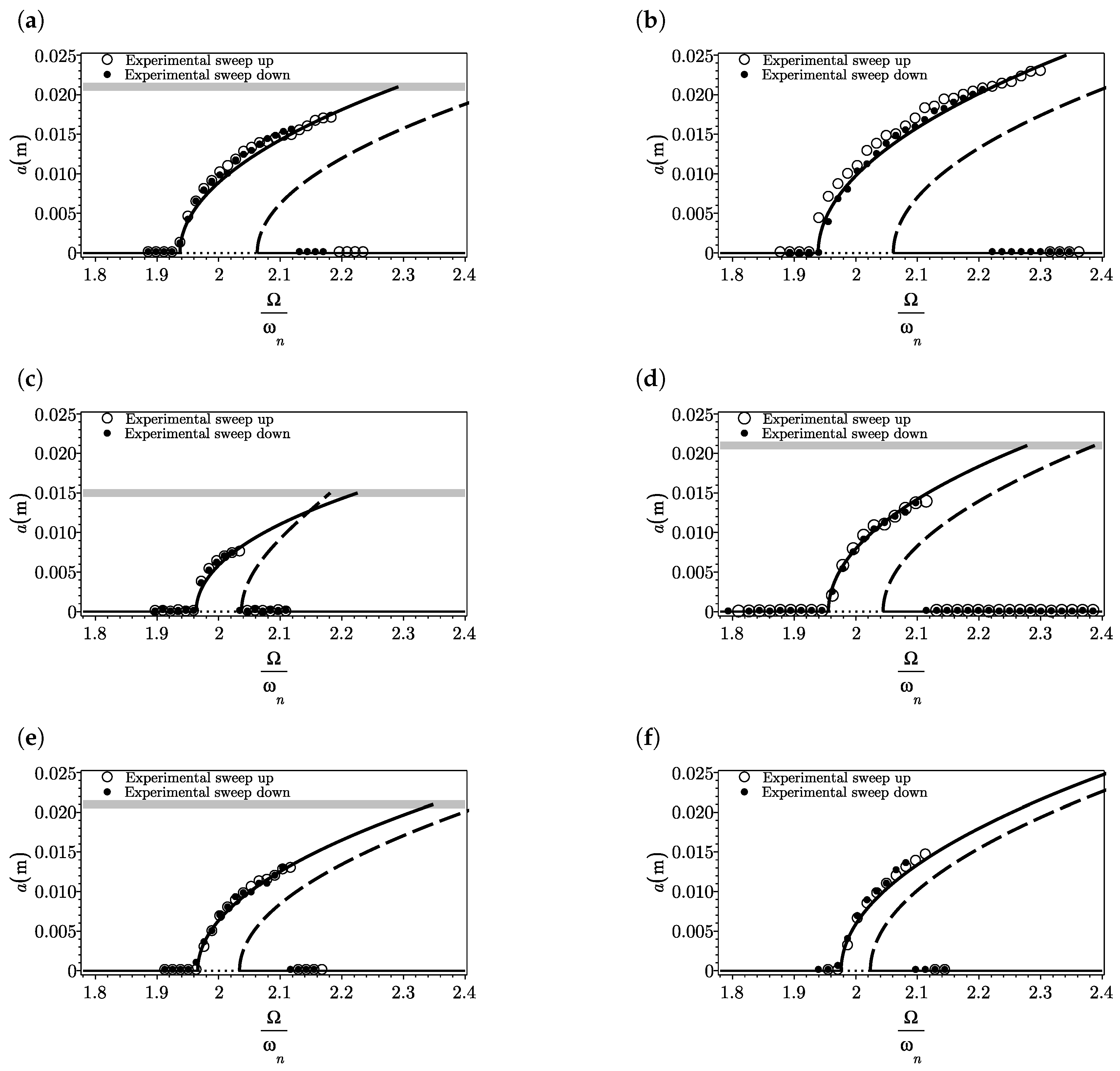
Figure 7 shows the theoretical $\frac{\alpha }{\delta }$ ratio for two direct and alternating currents in the coils. In each graph, two experimental cases are shown by the label ⨂ for two coil spacings h, when the $\frac{\alpha }{\delta }$ ratio is varied. To examine the robustness of the analysis the effect of cubic stiffness nonlinearity and parametric stiffness on response amplitude is tested at several positions.

Table 3. System parameters for experimental tests.

Tests	Measured Parameters					Calculated Parameters from Equations (23)–(28)
	h (m)	$I_{\mathrm{DC}}$ (A)	$I_{\mathrm{AC}}$ (A)	${\zeta }_{\mathrm{m}}$	${\omega }_{\mathrm{n}}$ ($\mathrm{rad}{\mathrm{s}}^{-1}$)	${\zeta }_{\mathrm{es},\mathrm{app}}$	${\delta }_{\mathrm{es},\mathrm{app}}$	${\gamma }_{\mathrm{es},\mathrm{app}}$	$\delta$	$\alpha$$({\mathrm{m}}^{-2})$	$\gamma$$({\mathrm{m}}^{-2})$
Figure 8a	0.03	0.92	0.14	0.001	48.60	146	17.44	24,761.7	0.129	1203.19	183.1
Figure 8b	0.035	0.97	0.155	0.001	40.12	60.16	8.93	11,188.82	0.122	956.40	152.82
Figure 8c	0.025	0.50	0.055	0.001	50.3	430.26	56.33	83,508.47	0.093	1262.17	138.83
Figure 8d	0.03	0.48	0.06	0.001	37.11	191.26	28.82	40,897.67	0.092	1055.86	131.98
Figure 8e	0.03	0.98	0.08	0.001	49.23	144.17	16.55	23,497.5	0.069	1214.5	99.14
Figure 8f	0.035	0.96	0.06	0.001	39.81	60.64	9	11,277.63	0.047	954.05	59.62

presents the system parameters for cases marked in Figure 7. From the result shown in Figure 7a, the $\frac{\alpha }{\delta }$ ratio at position $h=0.03\mathrm{m}$ is larger than that at position $h=0.035\mathrm{m}$. The amplitude-frequency plot for the two points marked in Figure 7a shows that, where the $\frac{\alpha }{\delta }$ is lower, the amplitude of the upper stable branch is higher. The jump frequency is lower when the cubic stiffness is greater. The amplitude-frequency plot is shown in Figure 8a for position $h=0.03\mathrm{m}$, and in Figure 8b for position $h=0.035\mathrm{m}$.

The cubic stiffness is maximized at coil spacing $h=0.025\mathrm{m}$ (Figure 7b). The amplitude-frequency curve at this coil spacing (Figure 8c) is compared with the amplitude-frequency at $h=0.03\mathrm{m}$ (Figure 8d). For all frequencies, the response amplitude for the case with higher cubic stiffness (Figure 8c) is smaller than the case with weaker cubic stiffness (Figure 8d).

Comparing the amplitude-frequency (Figure 8e,f) for the two coil spacings marked in Figure 7c shows that the amplitude of the response is greater at coil spacing $h=0.035\mathrm{m}$ for all frequencies, despite the slightly greater $\frac{\alpha }{\delta }$ ratio. The difference between the $\frac{\alpha }{\delta }$ ratio at a greater coil spacing has to be larger than at a closer coil spacing to significantly affect the amplitude of the response.

4. Conclusions

A nonlinear parametrically excited system has been analyzed, where the time-varying stiffness and nonlinear parameters were controlled by an electromagnetic subsystem. The experimental model, introduced in Section 2.1, was chosen because the parameters that define the system mathematically can be controlled independently. A mathematical model of this system was presented in Section 2, and was solved using the method of averaging. This model augments the models used in the literature by accounting for the cubic stiffness, cubic parametric stiffness, and nonlinear damping due to the induced current. This mathematical model was validated through experimental tests in Section 3.1.

Experiments determined that the system response is amplified at greater time-varying stiffness and cubic parametric stiffness due to parametric resonance. The nonlinear damping was included to model the effect of induced current in the electromagnets. Increasing the cubic stiffness attenuated the response and reduced the frequency bandwidth of the NPE system. The mathematical model accurately modelled the dynamics of the system for different coil spacings. Some small discrepancies between the analytical and experimental results remained, possibly due to the inclination angle between the magnets and the coils. This paper demonstrates that the effects of the nonlinear parameters are crucial for designing devices that can be modelled as nonlinear parametrically excited single degree of freedom systems, such as electromagnetic actuators, high pass filters, and amplifiers. The experimental results demonstrate that the augmentations made to the mathematical model are essential for describing the nonlinear behavior in these systems.

References

- Chivukula, V.B.; Rhoads, J.F. Microelectromechanical bandpass filters based on cyclic coupling architectures. J. Sound Vib. 2010, 329, 4313–4332. [Google Scholar] [CrossRef]
- Dohnal, F. Experimental studies on damping by parametric excitation using electromagnets. Proc. Inst. Mech. Eng. Part C J. Mech. Eng. Sci. 2012, 226, 2015–2027. [Google Scholar] [CrossRef]
- Faraday, M. On a peculiar class of acoustical figures; and on certain forms assumed by groups of particles upon vibrating elastic surfaces. Philos. Trans. R. Soc. Lond. 1831, 121, 299–340. [Google Scholar] [CrossRef]
- Rayleigh, F.L. On maintained vibrations. Lond. Edinb. Dublin Philos. Mag. J. Sci. 1883, 15, 229–235. [Google Scholar] [CrossRef]
- Zaghari, B.; Rustighi, E.; Ghandchi Tehrani, M. An experimentally validated parametrically excited vibration energy harvester with time-varying stiffness. In SPIE Smart Structures and Materials + Nondestructive Evaluation and Health Monitoring; International Society for Optics and Photonics: Bellingham, WA, USA, 2015; pp. 1–13. [Google Scholar]
- Rhoads, J.F.; Shaw, S.W.; Turner, K.L.; Baskaran, R. Tunable microelectromechanical filters that exploit parametric resonance. J. Vib. Acoust. 2005, 127, 423–430. [Google Scholar] [CrossRef]
- Welte, J.; Kniffka, T.J.; Ecker, H. Parametric excitation in a two degree of freedom MEMS system. Shock Vib. 2013, 20, 1113–1124. [Google Scholar] [CrossRef]
- Ghandchi Tehrani, M.; Kalkowski, M.K. Active control of parametrically excited systems. J. Intell. Mater. Syst. Struct. 2015, 27, 1218–1230. [Google Scholar] [CrossRef] [Green Version]
- Baskaran, R.; Turner, K. Mechanical domain non-degenerate parametric resonance in torsional mode micro electro mechanical oscillator. TRANSDUCERS 2003. In Proceedings of the 12th International Conference on Solid-State Sensors, Actuators and Microsystems, Boston, MA, USA, 8–12 June 2003; Volume 1, pp. 863–866. [Google Scholar]
- Abou-Rayan, A.M.; Nayfeh, A.H.; Mook, D.T.; Nayfeh, M.A. Nonlinear response of a parametrically excited buckled beam. Nonlinear Dyn. 1993, 4, 499–525. [Google Scholar] [CrossRef]
- Daqaq, M.F.; Bode, D. Exploring the parametric amplification phenomenon for energy harvesting. Proc. Inst. Mech. Eng. 2011, 225, 456–466. [Google Scholar] [CrossRef]
- Nayfeh, A.H.; Pai, P.F. Non-linear non-planar parametric responses of an inextensional beam. Int. J. Non-Linear Mech. 1989, 24, 139–158. [Google Scholar] [CrossRef]
- Daqaq, M.F.; Stabler, C.; Qaroush, Y.; Seuaciuc-Osorio, T. Investigation of Power Harvesting via Parametric Excitations. J. Intell. Mater. Syst. Struct. 2009, 20, 545–557. [Google Scholar] [CrossRef]
- Ghaderi, P.; Dick, A.J. Parametric resonance based piezoelectric micro-scale resonators: modeling and theoretical analysis. J. Comput. Nonlinear Dyn. 2013, 8, 011004. [Google Scholar] [CrossRef]
- Dolev, A.; Bucher, I. Tuneable, non-degenerated, nonlinear, parametrically-excited amplifier. J. Sound Vib. 2016, 361, 176–189. [Google Scholar] [CrossRef]
- Cugat, O.; Delamare, J.; Reyne, G. Magnetic micro-actuators and systems (MAGMAS). Trans. Magn. 2003, 39, 3607–3612. [Google Scholar] [CrossRef]
- Chen, C.C.; Yeh, M.K. Parametric instability of a beam under electromagnetic excitation. J. Sound Vib. 2001, 240, 747–764. [Google Scholar] [CrossRef]
- Yeh, M.K.; Kuo, Y.T. Dynamic instability of composite beams under parametric excitation. Compos. Sci. Technol. 2004, 64, 1885–1893. [Google Scholar] [CrossRef]
- Han, Q.; Jianjun, W.; Qihan, L. Experimental study on dynamic characteristics of linear parametrically excited system. Mech. Syst. Signal Process. 2011, 25, 1585–1597. [Google Scholar] [CrossRef]
- Kremer, D.; Liu, K. A nonlinear energy sink with an energy harvester: Transient responses. J. Sound Vib. 2014, 333, 4859–4880. [Google Scholar] [CrossRef]
- Verhulst, F. Nonlinear Differential Equations and Dynamical Systems; Springer Science & Business Media: Berlin/Heidelberg, Germany, 1996. [Google Scholar]
- Dohnal, F.; Mace, B.R. Amplification of damping of a cantilever beam by parametric excitation. In Proceedings of the CD MOVIC 2008, Munich, Germany, 15–18 September 2008. [Google Scholar]
- Zaghari, B. Dynamic Analysis of a Nonlinear Parametrically Excited System Using Electromagnets. PhD Thesis, University of Southampton, Southampton, UK, 2016. [Google Scholar]
- Nayfeh, A.H.; Mook, D.T. Nonlinear Oscillations; John Wiley & Sons: Hoboken, NJ, USA, 2008. [Google Scholar]
- Wheeler, H.A. Simple inductance formulas for radio coils. Proc. Inst. Radio Eng. 1928, 16, 1398–1400. [Google Scholar] [CrossRef]
- Sneller, A.J.; Mann, B.P. On the nonlinear electromagnetic coupling between a coil and an oscillating magnet. J. Phys. D Appl. Phys. 2010, 43, 295005. [Google Scholar] [CrossRef] [Green Version]
- Wei-Chau, X. Dynamic Stability of Structures; Cambridge University Press: Cambridge, UK, 2006. [Google Scholar]
Figure 1.
(a) Cantilever beam with a pair of identical magnets and a pair of identical coils on a wooden support. (b) Schematic model of the experimental set-up. A programmable power supply is used to generate controllable current from controlling input voltage. The vertical movement of the beam (in the direction perpendicular to both the x and z axes is minimized by precisely locating the beam between the axis of the two coils. This position is adjusted by entering the attractive mode, and then returning to the repulsion mode once the centered state is reached.
Figure 2.
(a) Schematic of the NPE oscillator. (b) Circuit diagram. Controllable power supply to generate current is connected to a resistor R and the coils.
Figure 3.
Diagram showing a pair of coils along with moving magnet in the center.
Figure 4.
(a) The analytical transition curve for a LPE system. (b) Analytical and experimental amplitude-frequency plot for a NPE system. Stable branches are indicated by solid lines, and unstable branches by dashed lines. The unstable trivial branch is shown by dotted line. The distance between the coils limits the maximum displacement of the beam to , shown by the grey line.
Figure 5.
Experimental results for point A in Figure 4b. (a) Measured displacement at the cantilever beam tip. (b) Current measured across the coils in series connection. (c) Power spectrum density (PSD) of the displacement signal. is at . (d) Power spectrum density of the current. (e) Phase portrait plot. (f) Poincaré map.
Figure 6.
Analytical and experimental amplitude-frequency plots. (a) Comparing solutions when and . (b) Comparing solutions of Equation (1) when , , and and when they are zero (indicated in grey). System parameters are presented in Table 2.
Figure 7.
The ratio between the cubic stiffness , and time-varying stiffness for different positions and input currents. (a) with high DC current, and high AC current. (b) with low DC current and low AC current. (c) with high DC current but low AC current. The ⨂ labels show positions, which are chosen to compare two cases in each individual graph with the current specified. The comparison is based on the amplitude-frequency plots shown in Figure 8. The “8a–f” annotations in the plots correspond to Figure 8a to f.
Figure 8.
Experimental and analytical amplitude-frequency plot. The system parameters are shown in Table 3. Stable branches are indicated by solid lines, and unstable branches by dashed lines. The unstable trivial solutions are shown by dotted lines.