

Modelling and Control of Longitudinal Vibrations in a Radio Frequency Cavity

School of Mechatronic Systems Engineering, Simon Fraser University, Surrey, BC V3T 0A3, Canada
*
Author to whom correspondence should be addressed.
Vibration 2024, 7(1), 129-145; https://doi.org/10.3390/vibration7010007
Submission received: 30 November 2023
/
Revised: 23 January 2024
/
Accepted: 24 January 2024
/
Published: 31 January 2024
Abstract
:Radio frequency (RF) cavities hold a crucial role in Electron Linear Accelerators, serving to provide precisely controlled accelerating fields. However, the susceptibility of these cavities to microphonic interference necessitates the development of effective controllers to mitigate vibration due to interference and disturbances. This paper undertakes an investigation into the modeling of RF cavities, treating them as cylindrical beams. To this end, a pseudo-rigid body model is employed to represent the translational vibration of the beam under various boundary conditions. The model is systematically analyzed using ANSYS software (from Ansys, Inc., Canonsburg, PA, USA, 2022). The study further delves into the controllability and observability of the proposed model, laying the foundation for the subsequent design of an observer-based controller geared towards suppressing longitudinal vibrations. The paper presents the design considerations and methodology for the controller. The performance of the proposed controller is evaluated via comprehensive simulations, providing valuable insights into its effectiveness in mitigating microphonic interference and enhancing the stability of RF cavities in Electron Linear Accelerators.
1. Introduction
Microphonic interference, primarily induced by environmental mechanical vibrations, can significantly affect the operational efficiency of superconducting radio frequency (RF) cavities within electron linear accelerators (e-LINACs). This phenomenon holds particular relevance to the ongoing construction of the Advanced Rare IsotopE Laboratory (ARIEL)(Vancouver, Canada) accelerator at TRIUMF(TRIUMF is Canada’s particle accelerator centre in Vancouver), which is Canada’s renowned particle accelerator center, as well as to other e-LINACs used around the world [1]. In an e-LINAC, the process accelerating electrons involve raising their energy levels up to 50 MeV while traversing a linear beam-line. This acceleration is achieved by utilizing RF cavity resonators, which propel charged particles forward by subjecting them to an oscillating electric field, commonly referred to as the accelerating field [2]. To deliver a high-quality beam, the bunched particles should receive the same amount of energy from the multi-cell RF cavities; therefore, the phase of the accelerating field should be precisely controlled. Well-tuned cavities assure good field stability; however, microphonic interference can create deformations in the cavity shape that can lead to shifts in the resonance frequency [3]. However, various studies to suppress mechanical vibrations have been conducted in the world’s accelerator labs [4,5,6,7,8]. Analytic solutions for RF fields in an RF structure have not been available, except for simple geometries. Also, an analytical model of mechanical vibration in a multi-cell cavity has not been available due to the complexity involved in creating such a model.
Further limitations in attempting to measure and control vibrations in TRIUMF’s nine-cell niobium cavity come from its boundary conditions. The cavity is suspended within a Helium bath with restricted access available only from the two ends. A structure without such boundary conditions would allow for the placement of sensors and actuators on individual cavities to measure and control vibrations [9,10,11,12]. In the case of the cavity at TRIUMF, we must contend with restricted ability to apply force to the cavity at both ends. Flexible structures are commonly used in a wide variety of engineering applications such as beams, rods, cables, plates, and cylindrical shells. These systems can be modeled by discrete mass and stiffness components and analyzed as multi-degree-of-freedom systems. Expressions for the natural frequencies and mode shapes can be derived for the classical homogeneous boundary conditions [13,14]. Various researchers have conducted studies on the free vibration of beams with uniform and non-uniform cross sections [15,16,17,18,19,20,21,22]. However, obtaining precise analytical solutions for the free vibrations of beams with varying mass and stiffness governed by differential equations is challenging. Exact solutions for rod vibrations are limited to specific beam shapes and boundary conditions. Thus, our objective is to create an appropriate working model to conduct free vibration analysis and then design a controller to control active vibration and noise. As such, the contribution of this paper is developing an observer-based controller that relies on the measurement of endpoint positions and tests it using an ANSYS model.
In this paper, we propose a novel approach to examine the flexural free vibrations of uniform beams, building upon previous research conducted by various scholars [23,24,25,26,27,28,29]. The organization of this paper is as follows. In Section 2, a model is presented for longitudinal flexural dynamics of a nine-cell cavity, such as that used in the e-LINAC as TRIUMF. This model incorporates a pseudo-rigid body framework to effectively capture the effects of microphonics and mechanical vibrations on the bending and stretching behavior of the cavity’s flexible structure. Subsequently, we derive the equation of motion for the developed model by employing the Lagrangian method. In Section 3, a comprehensive analysis of the cavity’s free vibrations is presented, employing a flexural uniform beam configuration with boundary conditions. Section 4 presents the design and introduction of an observer-based controller to mitigate the longitudinal vibrations within the cavity. In Section 5, the controller’s efficacy is demonstrated via rigorous simulations, showcasing its ability to effectively suppress undesired vibrations and enhance the overall performance of the system.
2. Longitudinal Flexural Dynamic Modeling
In our research, flexure and vibration are considered to be longitudinal, and lateral structural flexibility is neglected because the lateral vibration is not consequential to our specific noise cancellation needs (see Figure 1). The first step is obtaining the model’s Partial Differential Equation (PDE).
Considering the small element of the cavity, applied forces on the element, , and the element’s displacement, , is a function of the spatial and temporal coordinates (see Figure 1). Neglecting the higher order of deviations, the net force on the element with the width can be represented as
where denotes the partial derivation. According to (1) and Newton’s second law, the net force on an element is given as
where is the mass density, and denotes the beam cross section. Also, according to Hook’s law, the strain of an element along the x direction is calculated as
where denotes strain, and E is Young’s modulus. Calculating the derivative of (3) gives
Inserting (2) into (4) results in the wave equation as
The obtained wave equation must be satisfied over the entire beam domain, subject to the boundary and initial conditions. To solve (5), the variable separation method is used, i.e.,
where is the mode shape function, and is the temporal function, respectively, and they are independent. Inserting (6) into (5) gives the following equation
In order to satisfy this equation, both sides of (7) must be equal to a constant, e.g., , and give the following equation from the temporal function and for the spatial equation
The solution of (9) will provide proper mode shapes to be used in the Lagrangian method for obtaining the dynamic equation of the flexural beam. However, considering a beam with a non-uniform cross section makes (9) difficult to solve, and since the aim of the research is focused on vibration control, the authors assume a constant cross section for the beam. Thus, the longitudinal motion of the beam with an invariable cross section (i.e., A(x) = constant) is governed from (9) and is given as
where , which is the speed of the wave propagation in the tube. The general solution of differential (10) is therefore
To determine the integration variables and , various boundary conditions are applied and are presented in the following:
- (a)
- Free–Free Boundary ConditionThe boundary conditions are assumed to be free–free, i.e., at both ends of the beam, and the force is zero. Thus, the frequency and the mode shape function for this boundary condition can be defined as
- (b)
- Free–Fixed Boundary ConditionAssumes that the beam is fixed at one end and free at the other end. The frequency and mode shape, in this case, have been obtained as
- (c)
- Free-Ends-Fixed Middle Boundary ConditionAssumes that the beam is free at both ends but fixed in the middle. The dynamic is symmetric about the midpoint . For this type of boundary condition, the frequency and mode shapes are determined as
To sum up these three boundary conditions, Table 1 shows a summary of the frequency and mode shapes for these three boundary conditions.
3. Free Vibration Analysis
3.1. Energy Method
It is common to study the dynamics of flexible beam systems based on the Lagrangian equation. Equations of Motion can be written based on the Lagrangian equation, and boundary conditions are necessary to find the solution. The kinetic energy of a beam based on (6) is given as
where T represents the transpose operator. According to (18), the mass matrix, M, is given as
The potential energy is obtained according to (6) and is given as
The stiffness matrix, K, is given as
The Lagrangian equation results in the differential equations that describe the equations of motion of the system
where u is the input for the system.
3.2. Virtual Work
Considering as a generalized force, applying force u at x = 0, the virtual work can be calculated as
Applying virtual work in the boundary conditions, as presented, Section 2 results in a different input vector, b, according to the mode shapes.
Therefore, the equation of motion for this beam system will become the following
This model captures the dynamics of the system with sufficient accuracy by defining mass, stiffness, and also the input vector.
- (a)
- Free–FreeFor this boundary condition with a uniform cross-section dynamic, the mode shape function can be defined as (13). So, the generalized force function will be
- (b)
- Fixed–FreeFor this boundary condition, the mode shape function is defined in Equation (15), and the input vector is
- (c)
- Ends Free–Middle FixedIn this condition, the output of the system is a displacement function at point x = 0, and it is defined aswhere
3.3. Transfer Function of the System
To find the transfer function of the system, the first step is to write the system equation, Equation (25), in the Laplace domain
The output of the system from (29) in the Laplace domain is
Simplifying the system equation in the Laplace domain, the transfer function of the system is
Calculating the transfer function for the free–free ends boundary condition with the input vector, the transfer function results in the following:
In this method, if we assume that the beam is a uniform cross section, then M and K are diagonal matrices.
4. Controller Design
In this section, we present an overview of the controller design for active vibration and noise control systems. The control objective is to design the proper boundary control for suppressing the longitudinal vibration of the flexural dynamic.
4.1. Controllability
Lemma 1.
The system in (25) is controllable if mass and stiffness matrices (M and K) are symmetric, diagonal, and positive definite, and we assume that the boundary condition is either fixed–free or free–midway fixed.
Proof.
To prove the controllability of the system, considering the original system (25) and taking all the mentioned assumptions into consideration, we can therefore prove that the controllability matrix is full rank or rank() = 2n. The state space model of the system in (25) is
where , the A matrix, and the B matrix are
and the controllability matrix of the system is
To prove the controllability of the system, we should prove that the controllability matrix is full rank or = 2n. In order to calculate the rank of , we find the columns of the controllability matrix
Considering (40), in general, we are unable to demonstrate that is full rank, which means the system is not fully controllable (for all of its natural frequencies). In order to develop a controller, we typically first divide the system into controllable and non-controllable matrices. The controller is then designed to suppress vibrations in the controllable modes. However, for this specific dynamic and special boundary condition, assuming the mass and stiffness matrices as diagonal matrices, we can prove that is full rank and the system is controllable. The controllability Gramian of the system is defined as
□
Assuming that the mass matrix is symmetric, diagonal, and homogeneous, and the boundary condition is either fixed–free or halfway–fixed, we can write
where is a constant that relates to our matrix. This requires rewriting the controllability Gramian as follows
To prove that this specific dynamic is controllable, we need to prove that another equivalent system is controllable. Assuming a new system’s pair as () where and and the controllability matrix for this newly defined system is
, then it is full rank. Therefore, the newly defined system is controllable. On the other hand, the controllability Gramian of the new system is defined as
Considering , the relation between these two system Gramians is .
4.2. Lyapunov-Based Controller
Theorem 1.
The system introduced in (25) is asymptotically stable using the following controller
where γ is a positive gain and is replaced with an observer designed in section (observer design) as follows
where the matrix is
and the input to the observer-based controller is
Proof.
Defining the Lyapunov function of the system as , the derivative of this specified Lyapunov function candidate ( should be negative definite or negative semi-definite; thus,
If the input is defined as the multiplication of a negative value and the input b matrix and a derivative of the delta function
where is a positive gain, then the derivative of the Lyapunov function is
Therefore, the first derivative of the Lyapunov function is negative semi-definite, and the system is asymptotically stable. □
4.3. Observability
In this section, we show the system observability through a lemma, and then we proceed to design an observer-based controller.
Lemma 2.
The system in (54) is observable if K and M (stiffness and mass matrices, respectively) are symmetric positive definite matrices and the boundary condition is considered as fixed–free or free–mid fixed.
Proof.
Recalling the original system in (35), we can rewrite the system as
where
and the observability matrix of this system is
To prove the observability of the system, we should have = 2n that is full rank. The observability Gramian for our system is defined as
The system is observable if, and only if, is non-singular for any
We consider K and M as the symmetric positive definite matrix. To prove that Gramian is non-singular for all t, we must first consider defining a new pair as follows (), where and . This pair is observable; that is , where is the observability matrix for the new pair. To show this, we must obtain for the new pair
so (40) is also valid here and we can apply the same logic. The first two columns of are independent, so all other blocks of matrices are independent, and has a rank of 2n, so is observable. In other words, according to our definition, we have
We can write the observability Gramian for the newly defined pair as
Therefore, the Gramian matrix for the new pair becomes equal to the Gramian matrix of our original system pairs. When is full rank, and two Gramians are equal, therefore, is also full rank. This proves that the new defined pair is observable and so is our system □
4.4. Observer Design
The design of an observer to estimate the states of the system in order to design a controller is defined as follows.
Recalling the system output y from (29), the estimated output of the system is defined as
l is the observer gain vector defined as
where each and is an observer gain vector. The observer equation is
The new system’s equation with the observer will become the following
where
The estimation error of the states is written as
Therefore, the observer error system can be defined as
Using MATLAB (from Mathworks, Inc., Natick, MA, USA, 2022) to find mass and stiffness matrices numerically, it can be proven that the system is observable. Therefore, we can place eigenvalues of (67) in the LHP (left-half plane) as our observer pole placement and design our observer.
4.5. Observer-Based Controller Transfer Function
To find the overall transfer function of the system, the system needs to be considered as an equation
where y is input to the controller, and the observer gain vector is
Our observer-based controller system can be written in matrix form, defined as follows
where
The transfer function of the observer-based controller is
To calculate the transfer function of this observer-based controller, we need to find the determinant of the matrix.
This determinant is greater than zero; therefore, is invertible, and the transfer function can be calculated. Figure 2 illustrates the block diagram of the observer-based controller, in which the input u and output y are fed to the observer described by (71) with the control input specified by (72).
5. Experiment and Simulation Studies
In our experiment on the nine-cell Niobium cavities (manufactured and fabricated in PAVAC and TRIUMF, Vancouver, Canada) at TRIUMF, shown in Figure 3, we measured the vibration signal or phase noise from the cavity using a Spectrum Analyzer (Keysight Technologies, Santa Rosa, CA, USA).
As can be seen in Figure 4, some of the noise frequencies that we measured that caused the microphonics’ effect on the cavity’s signal are 20.332, 40.698 Hz, 46.077 Hz, 60.012 Hz, 124.664 Hz, 137.843 Hz, and 300.088 Hz. Given the limited availability of Niobium superconducting radio frequency cavities, or the limited time available to conduct experiments on existing cavities, it is challenging to experimentally develop a control system for them. The most straightforward and reliable way to design a controller for such a system is through simulation studies.
In order to simulate the nine-cell cavity at TRIUMF’s e-LINAC, we consider the superconducting cavity with its specific environment, that is, the cavity inside the injector cryomodule (EINJ), cooled down to 2 K. Considering this special setup of the cavity, in order to control the vibration of the cavity, we have some limitations in that we cannot attach any sensor or actuator attached to the body of the cavity because it is placed inside the Helium bath.
In our simulation studies, we utilize ANSYS from Ansys, Inc., USA, 2022, MATLAB (from Mathworks, Inc., USA, 2022), and SIMULINK software (from Mathworks, Inc., Natick, MA, USA, 2022). We use ANSYS for modeling, MATLAB for modeling and control designing, and we use SIMULINK to simulate the result of our proposed controller. In ANSYS Mechanical software, we import the actual geometry of the nine-cell cavity, and via finite element analysis, we find the eigenvalues of the system to calculate the Mass matrix and the Stiffness matrix.
5.1. Model Verification Using ANSYS Mechanical Analysis
Although, the actual structure of the cavity is more complicated and has both longitudinal and transverse vibration, in this study, we simplified the cavity structure as a uniform beam to focus our analysis and solution on only one dimension of the structure’s longitudinal vibration.
In this section, we use ANSYS software to perform modal analysis on the actual structure. In our modeling, it was helpful that we utilized finite element analysis using the ANSYS Mechanical interface. In this mechanical analysis, we set the model as TRIUMF’s nine-cell cavity structure, and the material has been set as Niobium. In the dynamic analysis for different boundary conditions, solving the modal analysis will result in different frequency solutions.
5.1.1. Free–Free Ends Model in ANSYS
Assume the cavity has two free ends and no fixed support. In general, for a free boundary condition dynamic, at least one zero natural frequency appears. The first six natural frequencies for this structure are shown in Table 2, Column 1. The first three modes in this Free dynamic are zero. The modes that affect the cavity in the x-direction are the modes that we are interested in controlling by adding external forces to both ends of the model. As an example of the Free–Free boundary condition’s natural frequency, a comparison between the original model and the displacement for the first mode in the x-direction is shown in Figure 5.
5.1.2. Midway–Fixed and Both-Ends-Free Models in ANSYS
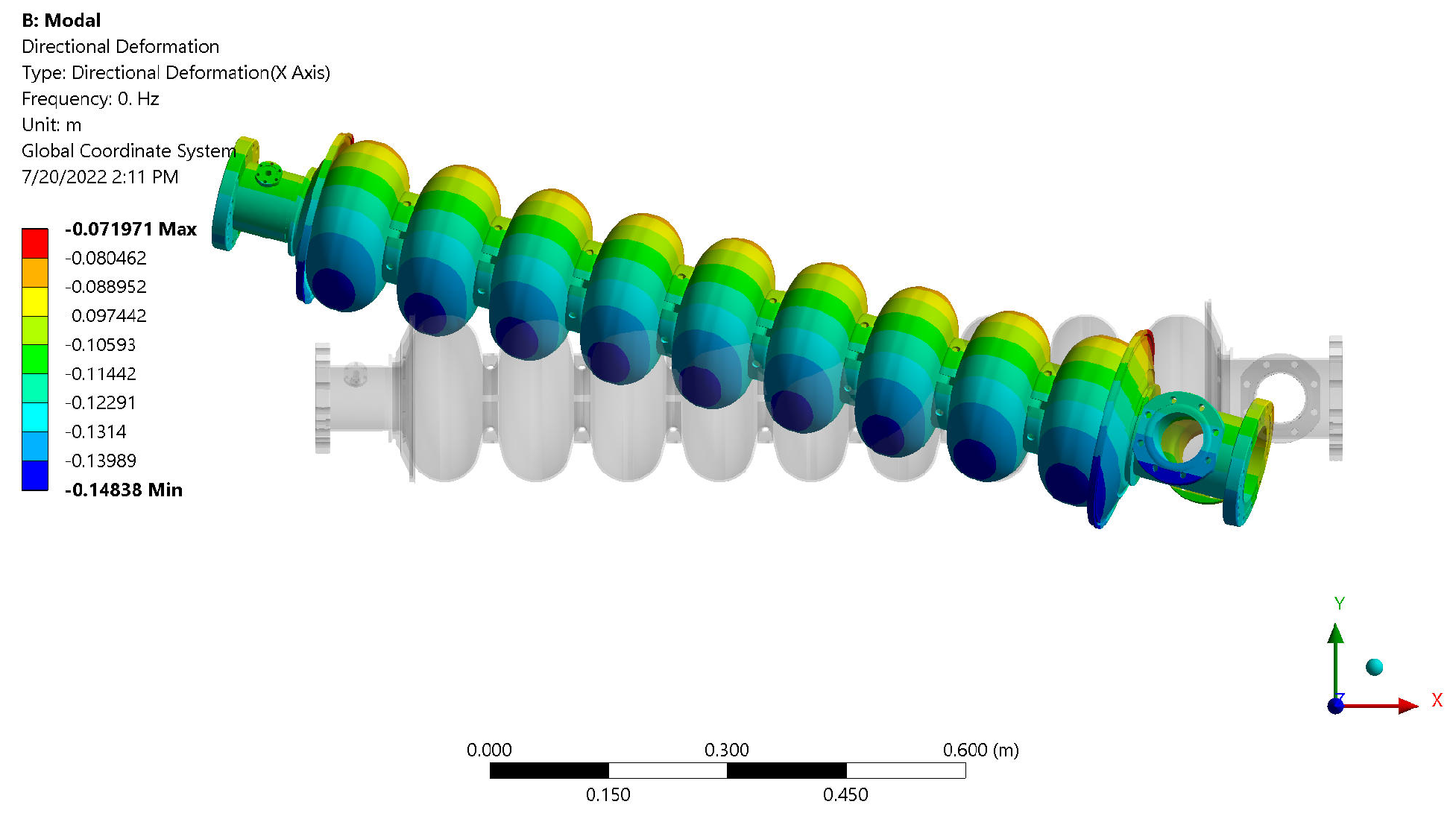
Assume the cavity is free at both ends but fixed in the middle. The cavity is symmetric about the midpoint . The force that the actuator should apply is assumed to be equally applied at both ends . By considering such a system, the only vibration that is controllable with the help of an actuator would be in the x direction; for example, the sixth mode is 140.107 Hz (see Table 2, Column 4). In Figure 6, the displacement for the sixth mode of vibration for this boundary condition is shown.
5.1.3. Fixed–Free Ends Model in ANSYS
Assume one end is free and the other end has fixed support. Therefore, at , there is no force, and we need to calculate the force value at to suppress the vibration and control the displacement. In this boundary condition, the values of the natural frequencies are half compared to the one that has two free ends (See Table 2, Column 5). As an example of this boundary condition, the displacement for the fifth mode of vibration is shown in Figure 7.
5.1.4. Fixed–Fixed Ends Model in ANSYS
Assume we have the cavity with two ends having fixed support. Therefore, six dominant frequencies for this cavity are presented in Table 2, Column 5. The modes that affect the cavity in the x-direction are the modes that we are interested in controlling by adding actuators to the ends of the model. In our ANSYS simulation, we observed that the mode that has the most displacement in the x direction in the fixed ends’ boundary condition is the fifth mode (see Figure 8).
5.2. Active Vibration Control Design in MATLAB
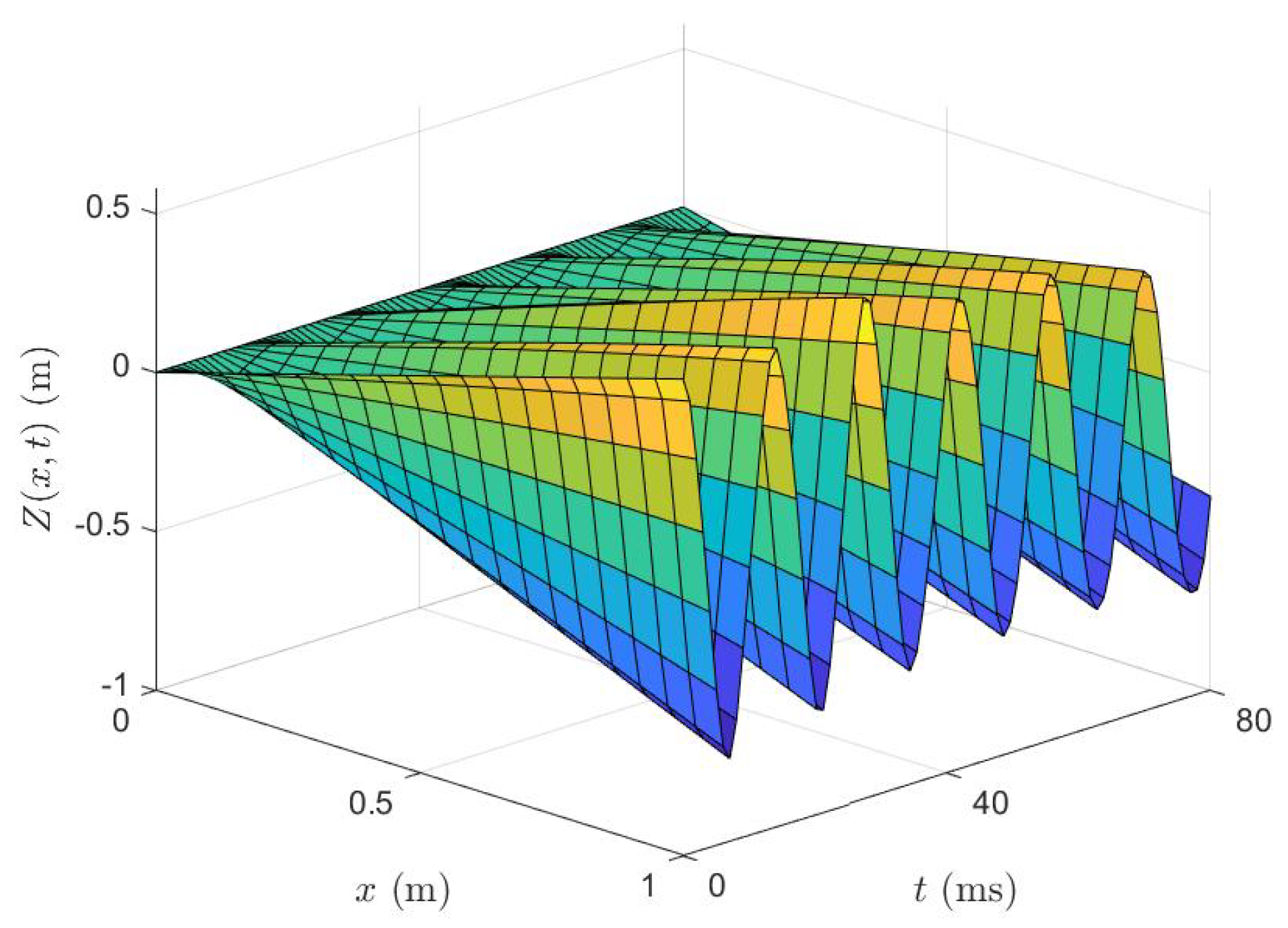
Our main focus in the cavity’s active vibration control is canceling the low-frequency longitudinal vibrations. Therefore, we just consider those first eigenvalues that are related to the longitudinal displacement of the cavity to build up the mass and stiffness matrices. After obtaining the reduced order mass and stiffness matrices of the cavity’s dynamic, we build a mathematical model for this simplified nine-cell cavity in MATLAB. The displacement of the endpoint in this simplified cavity without any control is shown in Figure 9.
In designing our controller, we are constrained by the superconducting cavity inside a 2 K Helium bath, meaning we only have access to both ends of the cavity to apply the actuator’s forces as our control signal. In this study, we developed an observer-based algorithm to cancel out the microphonic noises caused by the mechanical vibration activity. The control algorithm has been derived via a Lyapunov-based analysis. In the proposed observer-based controller, we considered the boundary condition resulting from the special situation that there is no access to the body of the cavity for placing the sensors and the actuators. The control design process consists of the use of a pure simulation environment based on MATLAB/SIMULINK, where the mathematical model includes a cavity model, an observer-based control system, and control strategies, considering the constraint in placing the actuator’s force.
In MATLAB, we design our proposed observer-based controller for this model, and in SIMULINK, we present the simulation results to evaluate the performance of the algorithms in canceling the microphonics. By applying the input signal to our model and closing the system’s loop through our proposed observer-based controller, we control the displacement function at the endpoint of our structure. Therefore, vibration in the endpoints of our structure has been suppressed for those specific frequencies that we designed our controller for (see Figure 10).
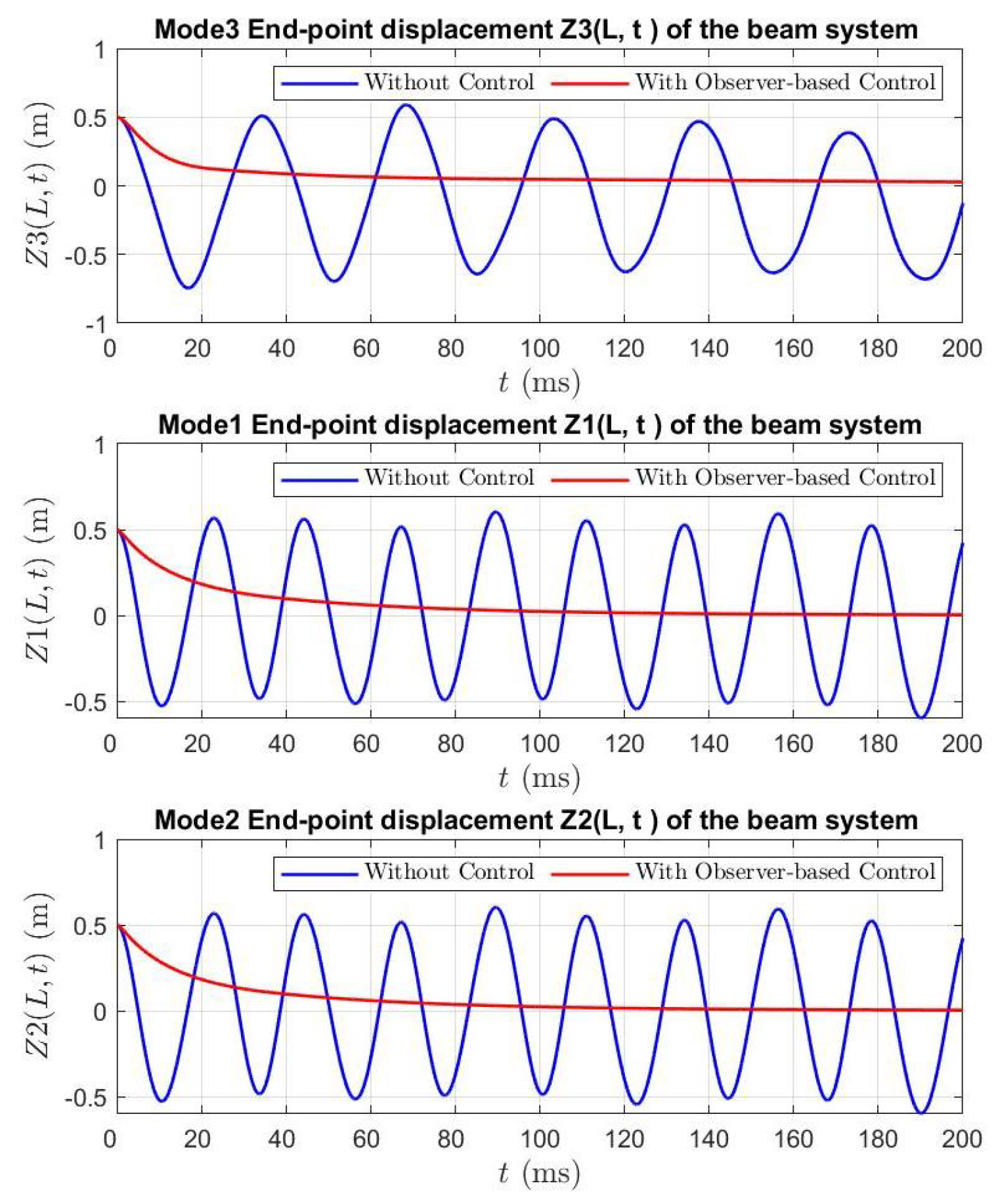
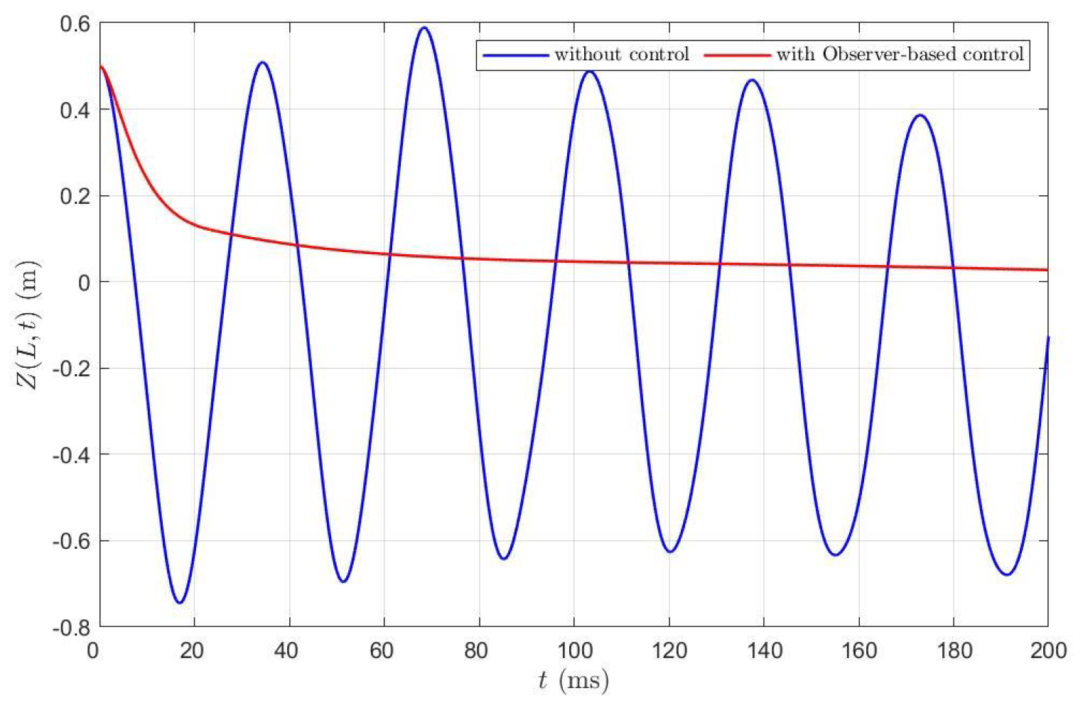
The control input signal is shown in Figure 11. In Figure 12, the displacement function for one of the modes without and with our controller is shown. The result shows that our proposed controller can suppress that vibration at the endpoint of the cavity’s model. Our proposed Lyapunov-based observer controller has been applied for three modes of vibration, and as has been shown in Figure 13, the controller cancels out those three modes of vibration for our simplified cavity model.
6. Conclusions
The flexural dynamics of a simplified nine-cell cavity modeled as a uniform cylindrical beam was studied in this paper, based on which a Lyapunov-based controller was developed for suppressing vibrations. A simulation study was conducted using ANSYS modal analysis to analyze the influence of boundary conditions on the natural frequency. By comparing the first six natural frequencies of the model under each boundary condition, it was observed that the absence of any fixed support results in specific natural frequencies being zero. When comparing the fixed-free, midway-fixed, and both-ends-free natural frequencies with those of the actual cavity model, the midway-fixed, both-ends-free modes closely matched the natural frequencies of the nine-cell cavity. The controllability and observability of the system were further investigated, leading to the development of an observer-based controller tailored for the system. The controller was simulated using MATLAB/SIMULINK and the results demonstrated the successful control of specific desired modes and the suppression of structural vibration.
Author Contributions
Conceptualization, M.K. and M.M.; methodology, M.K., M.M. and J.T.K.; software, M.K. and J.T.K.; validation, M.K., J.T.K. and M.M.; formal analysis, M.K., J.T.K. and M.M.; investigation, M.K. and M.M.; resources, M.M.; writing, M.K. and J.T.K.; writing—review and editing, M.M. and J.T.K.; visualization, M.K.; supervision, M.M. and J.T.K.; project administration, M.M. All authors have read and agreed to the published version of the manuscript.
Funding
This research was funded by Simon Fraser University and partially by TRIUMF Canada Particle Accelerator Centre.
Institutional Review Board Statement
Not applicable.
Informed Consent Statement
Not applicable.
Data Availability Statement
The data presented in this study are available upon request from the corresponding author. However, the data are not publicly accessible, in accordance with the policy of the Motion and Power Electronics Control Laboratory at Simon Fraser University, where the research was conducted.
Conflicts of Interest
The authors declare no conflicts of interest.
References
- Dilling, J.; Krücken, R.; Merminga, L. ISAC and ARIEL: The TRIUMF Radioactive Beam Facilities and the Scientific Program; Springer: Berlin/Heidelberg, Germany, 2014. [Google Scholar]
- Wangler, T.P. RF Linear Accelerators; John Wiley & Sons: Hoboken, NJ, USA, 2008. [Google Scholar]
- Kolb, P.U. The TRIUMF n.ine-c.ell SRF c.avity for ARIEL. Ph.D. Thesis, University of British Columbia, Columbia, UK, 2016. [Google Scholar]
- Arnold, A. Simulation und Messung der Hochfrequenzeigenschaften Einer Supraleitenden Photo-Elektronenquelle. Ph.D. Thesis, Universiät Rostock, Fakultät für Informatik und Elektrotechnik, Rostock, Germany, 2012. [Google Scholar]
- Marziali, A. Microphonics in Superconducting Linear Accelerators and Wavelength Shifting in Free Electron Lasers. Ph.D. Thesis, Stanford University, Stanford, CA, USA, 1995. [Google Scholar]
- Schilcher, T. Vector Sum Control of Pulsed Accelerating Fields in Lorentz Force Detuned Superconducting Cavities; Technical Report; DESY: Hamburg, Germany, 1998. [Google Scholar]
- Keikha, M.; Moallem, M.; Zhu, G.; Fong, K. Microphonic Noise Cancellation in Super-Conducting Cavity. In Proceedings of the IECON 2019-45th Annual Conference of the IEEE Industrial Electronics Society, Lisbon, Portugal, 14–17 October 2019; Volume 1, pp. 449–454. [Google Scholar]
- Keikha, M.; Kahnamouei, J.T.; Moallem, M. Radio Frequency Cavity’s Analytical Model and Control Design. Vibration 2023, 6, 319–342. [Google Scholar] [CrossRef]
- Alnuaimi, M.; BuAbdulla, A.; Silva, T.; Altamimi, S.; Lee, D.W.; Al Teneiji, M. Active Vibration Control of Piezoelectric Beam Using the PID Controller. In Proceedings of the ASME International Mechanical Engineering Congress and Exposition, Virtual, 1–5 November 2021; American Society of Mechanical Engineers: New York, NY, USA, 2021; Volume 85628, p. V07BT07A060. [Google Scholar]
- Shah, U.H.; Hong, K.S. Active vibration control of a flexible rod moving in water: Application to nuclear refueling machines. Automatica 2018, 93, 231–243. [Google Scholar] [CrossRef]
- Pham, P.T.; Nguyen, Q.C.; Hong, K.S. Vibration control of an axially moving beam attached to a translating base. In Proceedings of the 2021 International Symposium of Asian Control Association on Intelligent Robotics and Industrial Automation (IRIA), Goa, India, 20–22 September 2021; pp. 370–375. [Google Scholar]
- Pham, P.T.; Kim, G.H.; Nguyen, Q.C.; Hong, K.S. Control of a non-uniform flexible beam: Identification of first two modes. Int. J. Control Autom. Syst. 2021, 19, 3698–3707. [Google Scholar] [CrossRef]
- Koplow, M.A.; Bhattacharyya, A.; Mann, B.P. Closed form solutions for the dynamic response of Euler–Bernoulli beams with step changes in cross section. J. Sound Vib. 2006, 295, 214–225. [Google Scholar] [CrossRef]
- Kumar, B.; Sujith, R. Exact solutions for the longitudinal vibration of non-uniform rods. J. Sound Vib. 1997, 207, 721–729. [Google Scholar] [CrossRef]
- Zhou, D.; Cheung, Y. The free vibration of a type of tapered beams. Comput. Methods Appl. Mech. Eng. 2000, 188, 203–216. [Google Scholar] [CrossRef]
- Auciello, N.M. On the transverse vibrations of non-uniform beams with axial loads and elastically restrained ends. Int. J. Mech. Sci. 2001, 43, 193–208. [Google Scholar] [CrossRef]
- Eisenberger, M. Exact longitudinal vibration frequencies of a variable cross-section rod. Appl. Acoust. 1991, 34, 123–130. [Google Scholar] [CrossRef]
- Matsuda, H.; Sakiyama, T.; Morita, C.; Kawakami, M. Longitudinal impulsive response analysis of variable cross-section bars. J. Sound Vib. 1995, 181, 541–551. [Google Scholar] [CrossRef]
- Bapat, C.N. Vibration of rods with uniformly tapered sections. J. Sound Vib. 1995, 185, 185–189. [Google Scholar] [CrossRef]
- Lau, J. Vibration frequencies for a non-uniform beam with end mass. J. Sound Vib. 1984, 97, 513–521. [Google Scholar] [CrossRef]
- Abrate, S. Vibration of non-uniform rods and beams. J. Sound Vib. 1995, 185, 703–716. [Google Scholar] [CrossRef]
- Li, Q. Exact solutions for free longitudinal vibrations of non-uniform rods. J. Sound Vib. 2000, 234, 1–19. [Google Scholar] [CrossRef]
- Chen, L.Q.; Ding, H. Steady-state transverse response in coupled planar vibration of axially moving viscoelastic beams. J. Vib. Acoust. 2010, 132, 011009. [Google Scholar] [CrossRef]
- Zhang, Z.; Rustighi, E.; Chen, Y.; Hua, H. Active control of the longitudinal-lateral vibration of a shaft-plate coupled system. J. Vib. Acoust. 2012, 134, 061002. [Google Scholar] [CrossRef]
- Akgöz, B.; Civalek, Ö. Free vibration analysis of axially functionally graded tapered Bernoulli–Euler microbeams based on the modified couple stress theory. Compos. Struct. 2013, 98, 314–322. [Google Scholar] [CrossRef]
- Khot, S.; Yelve, N.P.; Tomar, R.; Desai, S.; Vittal, S. Active vibration control of cantilever beam by using PID based output feedback controller. J. Vib. Control 2012, 18, 366–372. [Google Scholar] [CrossRef]
- Parameswaran, A.P.; Gangadharan, K. Parametric modeling and FPGA based real time active vibration control of a piezoelectric laminate cantilever beam at resonance. J. Vib. Control 2015, 21, 2881–2895. [Google Scholar] [CrossRef]
- Sangpet, T.; Kuntanapreeda, S.; Schmidt, R. An adaptive PID-like controller for vibration suppression of piezo-actuated flexible beams. J. Vib. Control 2018, 24, 2656–2670. [Google Scholar] [CrossRef]
- Zhang, T.; Li, H. Adaptive modal vibration control for smart flexible beam with two piezoelectric actuators by multivariable self-tuning control. J. Vib. Control 2020, 26, 490–504. [Google Scholar] [CrossRef]
Figure 1.
Sketch of the cavity structure and forces acting on a flexural element (red arrows show the direcrtion of applied force on each element).
Figure 1.
Sketch of the cavity structure and forces acting on a flexural element (red arrows show the direcrtion of applied force on each element).
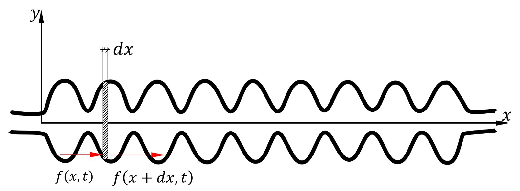
Figure 2.
Block diagram of the proposed observer-based control system.
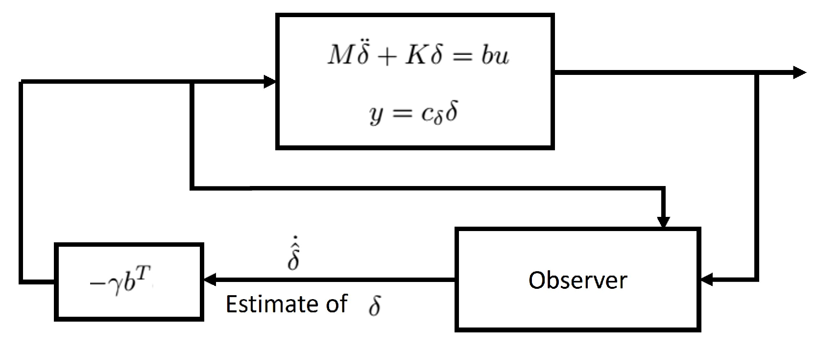
Figure 3.
TRIUMF’s nine-cell cavity structure.
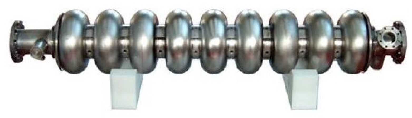
Figure 4.
Experimental vibration measurement data for TRIUMF nine-cell cavity (Yellow, Green and Purple sign waves show different vibration measurements).
Figure 4.
Experimental vibration measurement data for TRIUMF nine-cell cavity (Yellow, Green and Purple sign waves show different vibration measurements).
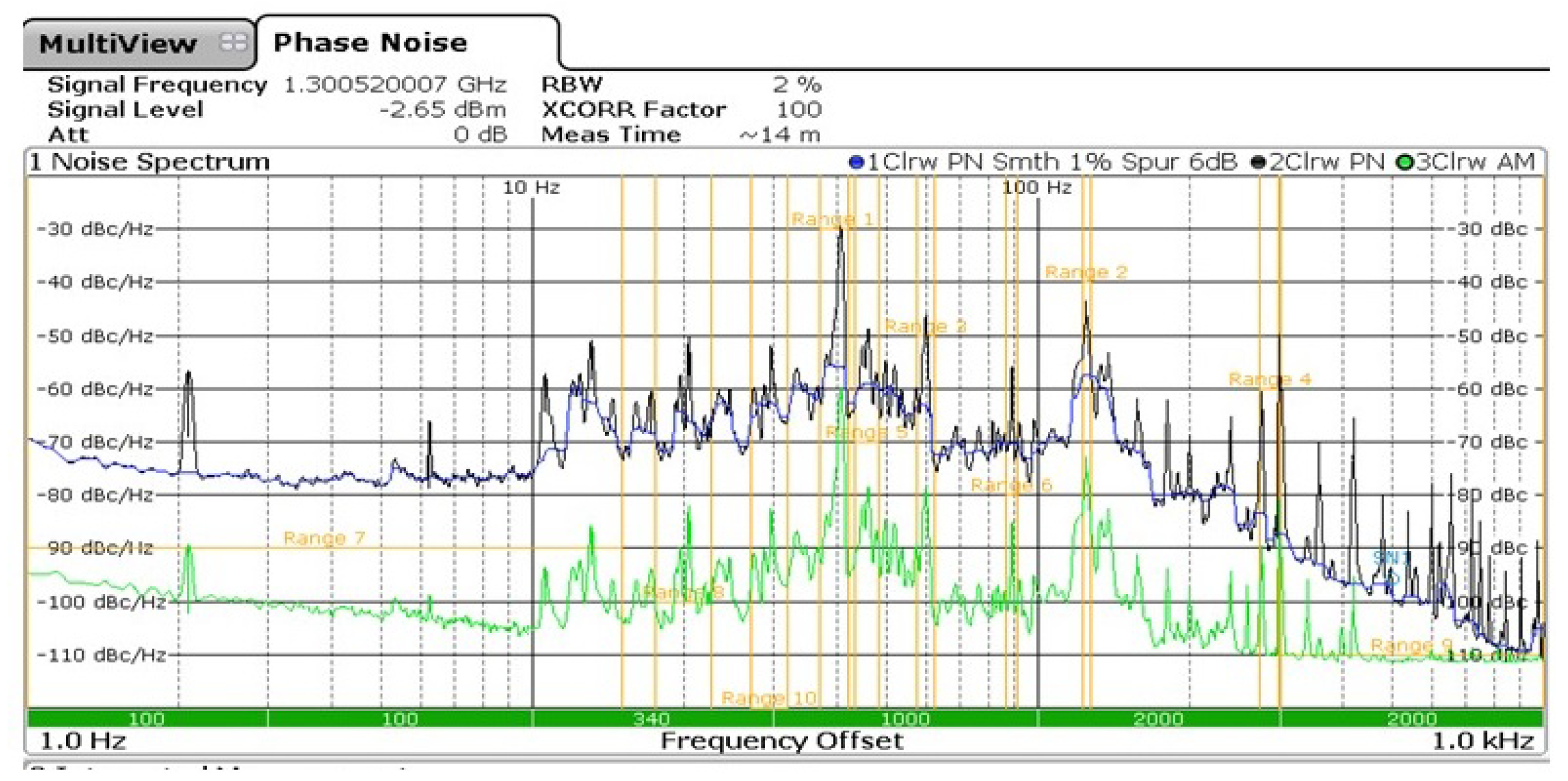
Figure 5.
ANSYS nine-cell cavity modal analysis for free–free boundary condition: Comparison between the original model and the first mode.
Figure 5.
ANSYS nine-cell cavity modal analysis for free–free boundary condition: Comparison between the original model and the first mode.

Figure 6.
ANSYS nine-cell cavity structure modal analysis for midway fixed and both ends free: Comparison between the original model and the displacement for the sixth mode in the x-direction).
Figure 6.
ANSYS nine-cell cavity structure modal analysis for midway fixed and both ends free: Comparison between the original model and the displacement for the sixth mode in the x-direction).

Figure 7.
ANSYS nine-cell cavity structure modal analysis for one end fixed and one end free: Comparison between the original model and displacement for the fifth mode of vibration).
Figure 7.
ANSYS nine-cell cavity structure modal analysis for one end fixed and one end free: Comparison between the original model and displacement for the fifth mode of vibration).
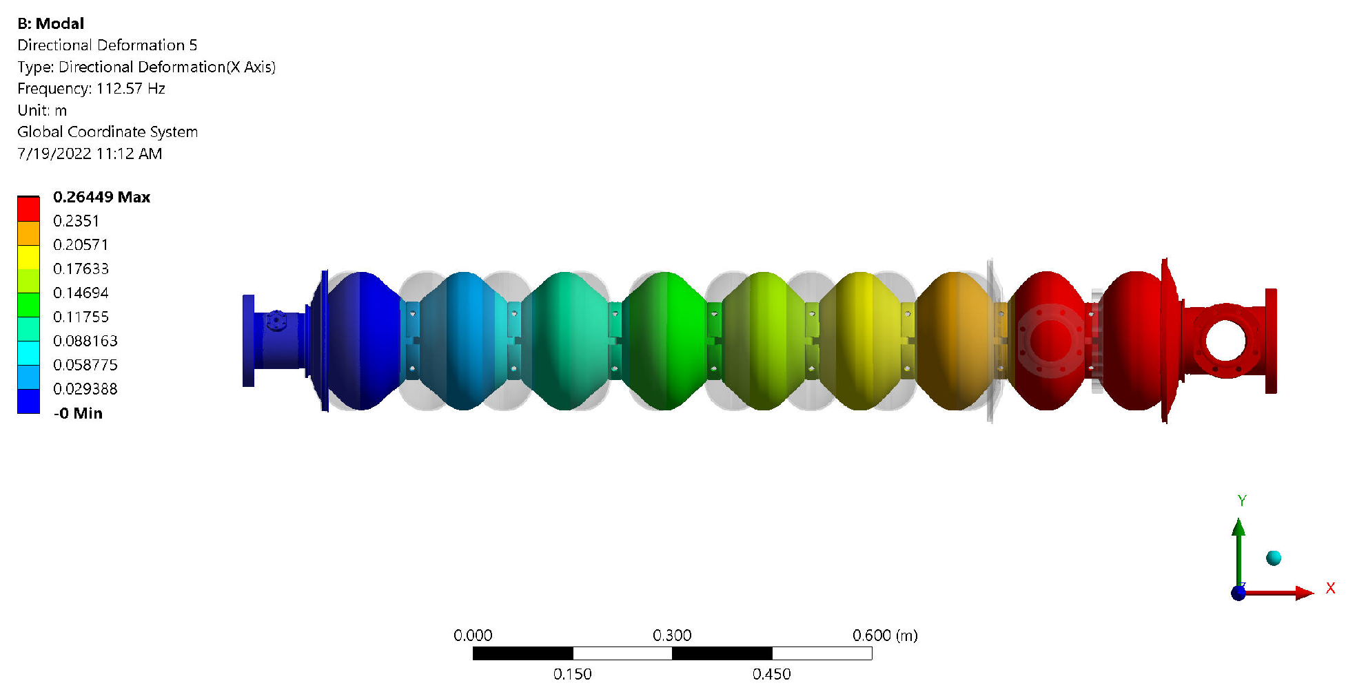
Figure 8.
ANSYS nine-cell cavity structure modal analysis for both ends fixed. The displacement has been shown for the fifth mode compared to the original model).
Figure 8.
ANSYS nine-cell cavity structure modal analysis for both ends fixed. The displacement has been shown for the fifth mode compared to the original model).

Figure 9.
Cavity flexural model endpoint displacement without control.

Figure 10.
Cavity flexural model endpoint displacement with observer-based controller.
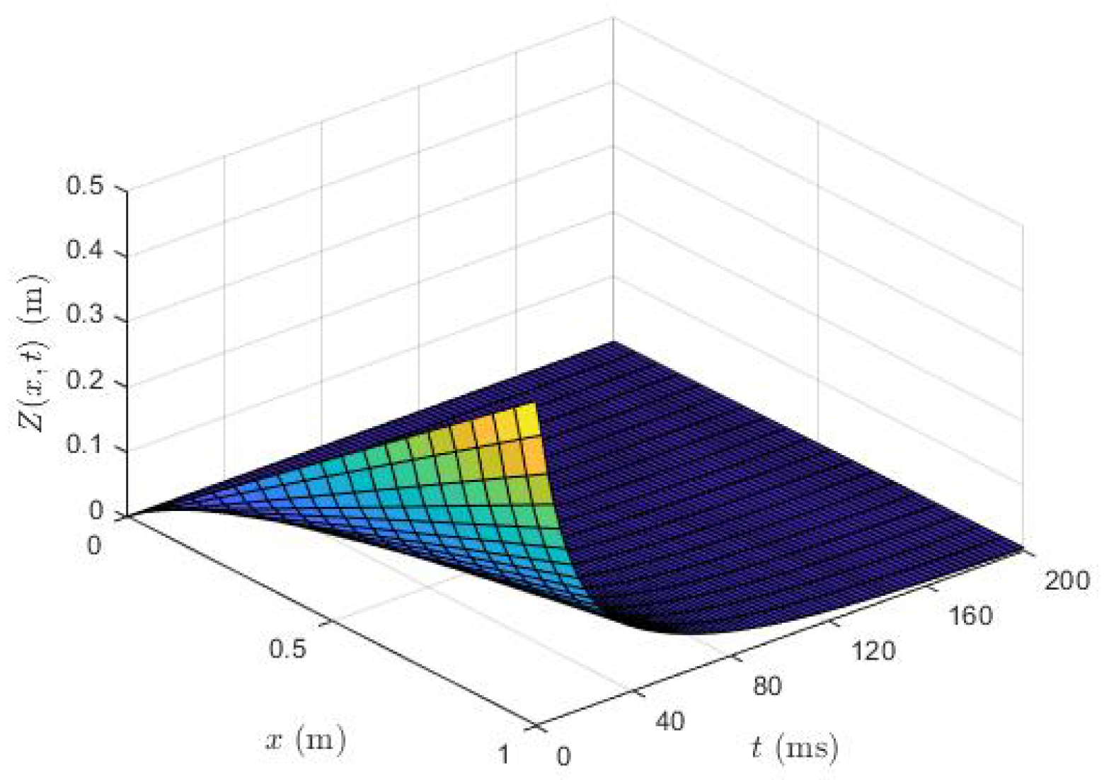
Figure 11.
Control input signal to the observer-based controller.
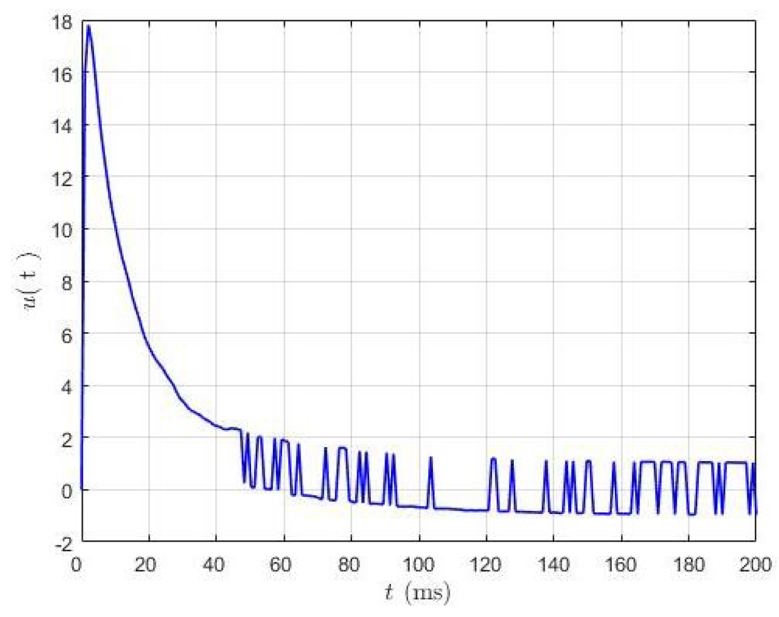
Figure 12.
Displacement function for the first mode at the endpoint of the model.

Figure 13.
Comparison of the displacement functions at the endpoint of the cavity’s model for three modes of vibration. Blue signals are displacement without control and the red signals are with observer-based control.
Figure 13.
Comparison of the displacement functions at the endpoint of the cavity’s model for three modes of vibration. Blue signals are displacement without control and the red signals are with observer-based control.

Table 1.
Different boundary conditions, frequencies, and mode shapes of a cylindrical beam.
| Boundary Condition | Frequency (rad/s) | Mode Shape |
|---|---|---|
| Free–Free | ||
| Fixed–Free | ||
| Free–Mid Fixed |
Note: *.
Table 2.
Cavity’s modal frequencies (Hz) in the x direction for various boundary conditions.
| Mode | Free–Free | Fixed–Free | Free–Mid Fixed | Fixed–Fixed |
|---|---|---|---|---|
| 1 | 0 | 8.64908 | 19.0875 | 82.049 |
| 2 | 0 | 8.81699 | 19.6901 | 85.962 |
| 3 | 0 | 56.8637 | 40.7481 | 200.68 |
| 4 | 47.396 | 59.1113 | 46.3741 | 200.47 |
| 5 | 49.182 | 112.567 | 127.646 | 299.59 |
| 6 | 129.69 | 153.406 | 147.42 | 342.29 |
Disclaimer/Publisher’s Note: The statements, opinions and data contained in all publications are solely those of the individual author(s) and contributor(s) and not of MDPI and/or the editor(s). MDPI and/or the editor(s) disclaim responsibility for any injury to people or property resulting from any ideas, methods, instructions or products referred to in the content. |
© 2024 by the authors. Licensee MDPI, Basel, Switzerland. This article is an open access article distributed under the terms and conditions of the Creative Commons Attribution (CC BY) license (https://creativecommons.org/licenses/by/4.0/).
Share and Cite
MDPI and ACS Style
Keikha, M.; Kahnamouei, J.T.; Moallem, M. Modelling and Control of Longitudinal Vibrations in a Radio Frequency Cavity. Vibration 2024, 7, 129-145. https://doi.org/10.3390/vibration7010007
AMA Style
Keikha M, Kahnamouei JT, Moallem M. Modelling and Control of Longitudinal Vibrations in a Radio Frequency Cavity. Vibration. 2024; 7(1):129-145. https://doi.org/10.3390/vibration7010007
Chicago/Turabian StyleKeikha, Mahsa, Jalal Taheri Kahnamouei, and Mehrdad Moallem. 2024. "Modelling and Control of Longitudinal Vibrations in a Radio Frequency Cavity" Vibration 7, no. 1: 129-145. https://doi.org/10.3390/vibration7010007