Non-Flat Earth Recalibrated for Terrain and Topsoil

Abstract

Earth’s land surface is raised from conventionally flat 15 Gha to >64 Gha accounting for hilly slope undulation and topsoil relief detail. Three main aspects are: topography, rugosity/tortuosity, and micro-relief/porosity of ice/vegetation-free ground. Recalibration arises from four approaches: First, direct empirical estimates of compiled satellite/LiDAR data means of +2.5–26% surface progressively overlain by +94% at cm² scale for soil ruggedness then +108% for mm² micro-relief; Second, from digital elevation models with thrice 1.6–2.0 times flat areas; Third, by ‘reverse engineering’ global soil bulk densities and carbon reserves requiring ×4–6 land. Finally, a Fermi estimation doubles the Earth’s surface—as exposed to Sun, air and rain—conveniently set at 100 Gha (with 64 Gha land:36 Gha ocean). Soil organic carbon (SOC) thereby grows to 8580 Gt mainly in SOM-humus with its biotic complexity plus roots, Vesicular-Arbuscular Mycorrhiza (VAM-fungi), leaf-litter and earthworms itself totaling 17,810 Gt. Although four to six times IPCC’s or NASA/NOAA’s calculated 1500–2300 Gt SOC, this is likely an underestimation. Global biomass and biodiversity are at least doubled (×2–3.5) and net primary productivity (NPP) increases to >270 Gt C yr⁻¹ due to terrain. Rationale for a ‘Soil Ecology Institute’ gains ground.

1. Introduction

This paper attempts to answer the simple question: “What’s the Earth’s true surface area?”. Surprisingly, this has no exact answer yet is key for determining the extent of the living world and it is crucial for understanding our planet’s essential life-support systems, especially the neglected soil. Even the most basic information on soils—upon which we live and depend for >99% human food [1,2,3], 100% timber and natural fibres, to filter all our drinking water, for medicines, such as Penicillins, Streptomycins, Malacidins and now Teixobactin or drugs, like Ivermectin (anti-parasitic) and Bleomycin (anti-cancer), and which support >98% of biota [4,5,6] (and herein) whilst also buffering pollution and climate change—is poorly known. For example: How much topsoil is there? What is its rate of production and loss? How about total soil biodiversity, primary productivity, and the principal vulnerabilities or extinction threats? Part of the reason for knowledge deficit is the lack of a single ‘Soil Ecology Institute’ comparable to myriad Marine, Aquatic, Atmospheric and Astronomical advocacy or research facilities around the globe (plus innumerable agriculture, chemistry, microbiology, or physics laboratories, albeit some claim a soil remit). A major oversight is ignoring terrain and topsoil, the main issue the current work confronts, as this graphic summarizes (Figure 1).

1.1. Land’s Surface Area

The present study builds on the author’s earlier work [2,7,8,9] and sources that are cited therein. Before focusing on topsoils/earthworms, it is necessary to first consider a broader picture and the implications of increasing land relief. By long-standing convention, land area is measured on a common surface plane projected onto the ground, i.e., as a two dimensional (2-D), flat, planimetric area. NASA/NOAA estimates are of 14.8–15.1 Gha land (29.2%) and 36.2 Gha ocean (70.8%) giving around 51 Gha for Earth’s (flat) surface [10]. However, these totals do not consider terrain, topography, nor rugged surface topsoil relief. In other words, they ignore that the ground is naturally hilly and soil bumpy. Reasoning from these Space, Oceanic, and Atmosphere agencies (everything but Soil?) is along the lines of the Globe being so large that slight elevations, such as the Alps, Andes, Antarctic Ranges, Atlas Mounts, Australia’s Great Dividing Range, Ethiopian Highlands, Himalayas, Japanese Alps and the North American Cordillera are insignificant. This may be essentially true at scales of observation around 10,000 km to 10,000 m (at which Ying et al. 2014 also found topography negligible, as is noted later). Under-appreciated is that while the sea is horizontally flat, land invariably undulates, and, since it indeed occupies only 29% of the projected surface, then the more planar versus hilly parts of just this proportion are inter-comparable. The following table summarizes the current false ‘flat-Earth’ status (

Table 1. Earth’s Inadequate Status Quo Flat-Earth Surface Model.

Flat Areas	CIA 2008 (Gha)	FAO (Gha) *	%
Six Continents	13.36	13.01	87
Antarctica	1.40 (2% ice-free)	1.4	9.4
Greenland	0.22 (21% ice-free)	0.18	1.2
Rivers/lakes	-	0.15–0.37	1.1–2.5
TOTAL	14.98	~14.96	100

* From Nunn & Puga (2009: appendix) [11] of ~15 Gha planimetric land including hot or cold deserts with roughly 80% (12 Gha) supporting terrestrial soils providing various levels of organic carbon, natural fertility and species richness; some bodies of water (e.g., temporary freshwater inundations, rice paddy, springs, bogs, marshes, or swamps) may yet be classed as having wetland soils or non-marine sediments.

).

While flat planimetric areas are suitable for administration, they are inapplicable for ecology. Under that worldview, the land seems relatively unimportant when compared to oceans and the current disparity for soil ecology is such that the World Scientists’ Warning to Humanity [12] originally from the majority of science Nobel laureates (most of whom were unqualified to comment since there is yet no prize for Applied Ecology) notes that: “the loss of soil productivity was listed as a concern in the 1992 scientists’ warning, but this variable was not analyzed here due to a lack of global data on changes in soil productivity”. Neither were their issues “ in order of importance or urgency”. Similarly, the UN’s 17 Sustainable Development Goals (from UN 2015 “2030 Agenda”—un.org/sustainabledevelopment/sustainable-development-goals/) overlook soil or earthworms as major considerations, citing “soil” but twice under “Goal 15: Life on Land”.

1.2. Global Triage

Applied Ecology (a mostly unrecognized form of environmental triage [13]) is needed to identify critically threatening issues or deficiencies and to provide clear direction for effective treatments or resolution. Triage cares not about past happenings nor distant possibilities, just the most immediate concerns. A recent review of planetary support systems [14] may be taken as an initial step. Yet, whilst ocean acidity was catalogued, the more rapid and urgent soil acidification (up to six times more severe than in the sea, see [15]) was ignored, as were topsoil erosion and salinity/sodicity issues. Overlooked also was soil microplastic pollution that was estimated at four to 23 times higher than the much publicized marine problem [16]. Moreover, Rockström et al. [14] and others were criticized for failing to adequately evaluate soils as Koch et al. (2013) summarized [17]: “Discussions around biodiversity loss seldom refer to soil even though soil contains the most diverse and complex ecosystems on the planet. Soils contain over 98 per cent of the genetic diversity in terrestrial ecosystems (Fierer et al., 2007) however soil biodiversity is not addressed in the Global Biodiversity Outlook (GBO-3) from the UN Convention on Biological Diversity (Secretariat of the CBD, 2010), and is not referred to in the popular International Union for Conservation of Nature (IUCN) Red List of Threatened Species (IUCN, 2012). Recent attempts to develop a global framework for assessing planetary resources also fail to recognize the vital role of soil in the biosphere... (Rockstrom et al., 2009). This important work is influential in current reviews of sustainable development, but does not address soil as a critical contributor to buffering the thresholds of those boundaries”. Rather, the current report demonstrates that soil, with earthworms, provides a foundation for all pillars of support for ‘Life Systems on Earth’, including those in the sea (Figure 2).

Two millennia ago, Aristotle concurred with Plato in recognizing that soil erosion with loss of humus and earthworms due to soil erosion around Athens from forest clearance and overgrazing was catastrophic to civilization [19]. Still highly pertinent today as certainly the most urgent of all the social, economic, and ecological problems is the loss of our precious topsoil. This is estimated, based upon United Nation’s FAO (Food and Agriculture Organization) data from Pimental & Burgess (2013) [3], to occur at a rate of 75 billion tonnes lost per annum, or 2000 tonnes per second worldwide [9]. For vital soil organic carbon alone, Duursma & Boisson (1994: fig. 14) [4] tallied 400–500 million tonnes run-off via rivers to the ocean per year (=~1 Gt humus lost at 30 t per second). Combining these two data confirm a reasonable humic soil organic matter (SOM) content as 1.3% (1 Gt SOM in 75 Gt eroded topsoil on a dry weight basis), as will be discussed later with bulk density.

Erosion provisions and poisons seas. Moreover, the erosion of chemically contaminated agricultural soil is often orders of magnitude greater than natural soils hence, rivers are brown and silted and the air dusty in farming regions and some farms may have just 12 year’s soil remaining [9]. For broadacre farmlands, the situation is so dire overall that UN’s FAO predicts only another 50 years of harvests [20]; similarly, in China [21] or the United Kingdom (UK) [22], it is particularly bad in India and seemingly disastrous in Africa and the Americas [3,15]. It is further reported [3] that 80% of the world’s agricultural land suffers moderate to severe erosion, and, in the last 40 or so years, about 30% of farmland was abandoned after becoming unproductive. Erosion rates, if from ‘flat-Earth’ models, will also require elevating for terrain and relief.

1.3. Vital Global Resources

Basic requirements for continued humanity or other higher life are: healthy soil, water, and air. Oxygen is needed in scale of seconds, freshwater every few hours, and food daily, along with habitat or shelter under ecological infrastructure support. Smaller organisms, juveniles, or invertebrates need lower supplies but more constantly. Often the most limiting of factors relate to primary productivity as tallied in this table (

Table 2. Primary Productivity (P.P.) in Terms of Organic C and O₂ Production.

P.P.	Area Gha	Org-C g/m2/yr	Total Org-C Gt/yr	O2 g/m2/yr	Total O2 Gt/yr
Land	15 *	144	21.6 (46%) *	384	57.6 (44%) *
Ocean	36	72	25.9 (54%)	206	74.3 (56%)
TOTAL	51 *		47.5 (100%) *		131.9 (100%) **

Compiled from Duursma & Boission (1994: tab. 2) [4]. * Land area is contested in the present work allowing its productivity to be at least doubled. ** It is nonsense to claim “oceans provide every second breath of air” because a massive atmospheric O₂ reserve is 1.2 million Gt thus 131.9 Gt annual photosynthetic contribution from soil & sea combined is just 0.01% per year and turnover time for O₂ is in the order of 10,000 yrs—a literal ‘drop in the ocean’. Twenty-five years ago, Duursma & Boisson (1994: 135) [4] reported that oceans contain only 0.22% of global living biomass (99.78% on land).

).

Oxygen, which is necessary for most organisms to respire, is depleted by 99.2% at the air/water boundary, yet it percolates throughout the soil to depth, as with rainwater, due mainly to the burrowing of earthworm. These carbon productivity calculations have increasingly been revised upwards, recognizing the land’s larger role. Productivity values given by other authors (Whitman et al. 2008: tab. 6) [23] are twice as high at 99 Gt total per year, whilst the satellite-derived Normalized Difference Vegetation Index (NDVI) [24,25] have 105 Gt (54% from land) and 170 Gt per year (68% from land), respectively. Most recently UNEP (2002: tab. 1.1) [26], has Ocean vs. Land of 48.5–83 vs. 56.4–90 Pg C (totals 105–173 Gt C) (cf. Figure 3).

Life on Earth is mainly provided for by primary productivity on land that operates at the biological scale of a plant’s leaf or seed, of an earthworm’s burrow/castings or cocoon: at around the centimetre to millimetre level. Average leaf size reportedly ranges from 0.011 to 39.5 cm² [28], while an earthworm’s burrow or cocoon are about 0.1–1.0 cm in diameter [29]. However, the true extent of total topographical topsoil that actually supports land plants and hosts earthworms is wanting.

1.3.1. Neglected Soils and Earthworms

Currently, no finer resolution than kilometres, at best, seems applied to a flat global surface area of soils resulting in the following incorrect model overemphasizing the ocean (Figure 4).

Food overwhelmingly comes from earthworm-rich topsoils that are being rapidly depleted by agrichemical farming [15]. Darwin (1881: 173) [31] estimated that earthworms annually eject in the order of 15 tons per acre of surface castings on pasture/commons land (=33.6 t ha⁻¹ yr⁻¹), whereas Lee (1985: tab. 18) [29] has optimal mean of 105 t ha⁻¹ yr⁻¹ (× 9.5 Gha of non-ice/non-desert land = 998 Gt yr⁻¹ globally). Conversely, UN-FAO (2015: 103) [32] estimates global soil formation now as just 0.15 t ha⁻¹ yr⁻¹, while the rate under agricultural conditions ranges 0.5 to 1 t ha⁻¹ yr⁻¹ or at most 1 × 9.5 Gha = 9.5 Gt yr⁻¹. This compares to topsoil loss of 75 Gt per annum [3]. Following Darwin, it is generally accepted that earthworms are the major contributors to rebuilding or maintaining fertile and well-drained soil [29,33]. However, their rate of replacement cannot keep pace under relentless cultivation and poisoning due mainly to increasingly intensive chemical agriculture that depletes both topsoil and biodiversity. Not only populations are declining at alarming rates, several neglected earthworm species are also now extinct or likely soon to be (e.g., [34,35,36] and the author’s unpublished data).

When these vital topsoil builders are gone, then every other organism on this planet suffers.

1.3.2. The Scale of Topsoil Biodiversity

The majority of deep carbon in soils is stored as SOM-humus composed of earthworm casts, decaying plants and both living and dead (or dormant) animals, fungi, and microbes. One cubic metre of soil ideally supports ~200,000 arthropods, ~2020 true megadrile earthworms (~305 gm⁻²), countless other larger or lesser organisms, plus up to 112 km m⁻² of fine-roots in just the top 30 cm (Lee 1985: tab. 7) [29,37]. A single gramme (~1 cm³) of fertile topsoil may have three billion microbes (Bacteria, Actinomycetes, Archaea, Fungi, Protozoa, etc.), up to 60 km of fungal hyphae, with 10,000 to 50,000 microbial species having 1598 km of DNA some dating to the beginning of life four billion years ago [3,5,38,39]. Soil biodiversity and food-web interdependence are layered and complex (Figure 5). However, all biotic totals are underestimated without terrain at scale and depth.

1.4. Aims of this Study

This project aims to determine the true extent and nature of global topsoil. Despite depletion, biota-supporting topsoil is yet key for regulation of atmospheric gases (e.g., CO₂, N₂O, CH₄—[38,41]), it underpins primary production plus its humus is the interface of adsorption/retention/rehabilitation of pollutants, such as heavy metals and pesticides. It supplies sustenance and medicines (as indeed do earthworms—[42]). Due to this dependency, importance, and urgency, one would think that the status of soil is well worked out as a major concern. In fact, the opposite is true and more is known about the relatively unproductive and unpopulated oceans or the status of inert dirt on other planets than of the living topsoil on habitable Earth. Inexplicably, the less critical spheres of air, water, and even outer Space are most exquisitely plotted and their research is well supported by long-term projects extending far into the uncertain future.

The present study provides some initial direction to help redress this unfathomable imbalance of an abysmal lack of knowledge of soil ecology or basic information on the terrestrial soil biome. It does not provide a definitive answer to the total surface area of land or volume of topsoil: rather, it indicates a framework for estimates and raises questions to the lack of previous approximations for these essential data. The topsoil too may require broad re-evaluation and protection due to its high primary productivity, moisture relations, and gaseous exchange at the interface between all three key elements (viz. soil, water, and air) in its living SOM humus—the last and least well-known biotic frontier (http://science.sciencemag.org/content/304/5677), on which our knowledge needs to boldly grow. Quoting from Prof. J. Bouma [43]: “every soil has a story to tell, a fascinating story of how she was formed and how she functions in terms of potentials and limitations”.

2. Materials and Methods

2.1. Theoretical Basis: Digital Elevation Models (DEMs)

Aspects of three-dimensional (3-D) terrain and scale are presented by Kamphorst et al. [44]. Regarding the extent of the true land surface on Earth the data is currently unavailable, even standard definitions of the various Digital Elevation Models (DEMs) are wanting. Despite global initiatives (such as the http://globalsoilmap.net/) and a growing number of local topological projects at finer scales, a unified global terrain data set remains, nonetheless, elusive due to several factors: “largely the result of technical challenges to sharing very large data sets and issues of data ownership and permissions” [45]. Methodologies and technology are under development but when high resolution satellite radar data, now available only to the military for resource competition, becomes more generally available then accurate assessment of soil roughness over much larger surface areas will be calculable by geo-morphologists for use by succeeding soil-ecologists.

Theoretical terrain DEMs include DSM, a Digital Surface Model representing Earth’s surface including all structures upon it, in contrast to the Digital Terrain Model (DTM) that represents bare ground without any objects like snow, plants or buildings (Figure 6).

Essence of the present study is that compiled data for neither DSMs nor DTMs seem available.

2.2. Satellites and LiDAR (Laser Light Detection And Ranging)

This topography deficit is surprising as the Landsat programme started in 1972 and the most recent Shuttle Radar Topography Mission (SRTM) was from 2000. Different technologies (as presented by www.charim.net/datamanagement/32) have LiDAR the most accurate, but least extensive, at scales 0.5-m or less. Nevertheless, some countries already have complete coverage from satellite data, e.g., for Australia, China, Czech Republic, Denmark, Japan, Macedonia, and the USA. The UK’s Environment Agency has LiDAR DEMs for much of England most in 1–2-m resolution, some 50–25-cm (http://vterrain.org/Locations/uk/); initially, “data for the whole country costs £56,250 plus VAT(!)” although increasingly it is free. Unfortunately, few data are compiled into useable summaries, ideally of vegetation-free surface areas using high definition single photon LiDAR.

An uncompiled data set has been released with a one arc-second, or about 30-m courtesy of NASA (www2.jpl.nasa.gov/srtm/). The Japan Aerospace Exploration Agency (JAXA) released “ALOS World 3-D—30 m (AW3D30)”, a global digital surface model (DSM) dataset with a horizontal resolution of ~30-m mesh (1 × 1 arc-second), free of charge, in May 2015. Another estimation of bare-earth from USDA removes vegetation from satellite data (available from USDA: https://naldc.nal.usda.gov/download/38817/PDF), although this too has no total topography data.

Methodology is provided [46] as a practical example of the surface to horizontal areas. The entirety of Garrett County, MA, USA, was mapped covering a flat 1700 km² area but enquiries of the authors for terrain totals were unforthcoming. A demonstrable image is self-explanatory (Figure 7).

2.3. DEM Errors and Straight Line Underestimations

For macro terrain a need is to find 3-D surface area to 2-D planimetric area ratio of a mapped topographic surface. A summary by Jenness (2004: 830) [47] says: “Hodgson (1995) [48] demonstrated how most slope-aspect algorithms generate values reflecting an area 1.6–2 times the size of the actual cell”. Jenness mapped an area of USA of 54,850 km², but seem not to provide 3-D data for this. His broad computation model is shown compared to actual biotic elements such as worm casts (Figure 8).

A 3-D Tortuosity index is T_i = TSA/TMA where TSA = Total Surface Area, TMA = Total Map Area at specification (subscript i), but often only linear profile ratios are made of surface relief by a flat Euclidean line (L1/L0), thus no account is taken of curved or irregular arcs nor hollows. A major problem with slope approximations, depending upon the algorithm used, is that ascendancies may be cancelled by declines, and vice versa, plus the slope aspects are random and irregular with regards to any fixed compass point adding yet more complexity. In other words, slope summaries are likely to be considerable underestimations at both larger and smaller scales, and natural curves or convoluted distortions of detail features are also unaccounted for by most models. Potentially more accurate are actual, on-the-ground, laser survey compilations. Microrelief may be additionally overlooked as a constant error in most DEMs (Figure 8).

Some of the concepts as proposed and newly applied in this paper are illustrated (Figure 9).

Quadrat surveys on slope may underestimate areas. Micro-relief requires consideration too as, for instance, earthworm superficial castings from subterranean burrowing at the cm² or less scale in a 1 m² quadrat would be a factor for surface relief calculations. This especially since one square metre of savannah or pasture may have 200–600 casts m⁻² or even be completely composed of casts to some depth, from a network of up to 888 m/m² in the length of burrow systems (=8880 km/ha) (from Lee, 1985: 90, 183, 196) [29,49]. Thus, depending upon objectives of a study, overlooked terrain and rugosity may underestimate results, and, even if flat spots are chosen for survey points, this ignores the surrounding slope effects introducing yet other errors.

The issue of quadrat under-sampling errors with a worked example of terrain (of Mt Fuji) and three soil area analogies (paint, kimono, and the ‘Coastline Paradox’) are presented in Appendix A.

2.4. Appropriate Scales

Mega scale (km) is only appropriate for astronomy or hydrology. Three apparently valid finer distinctions that relate to scales of observation on land are: topography, soil tortuosity, and soil surface micro-relief. Super- or sub-imposed on these is fractal porosity of topsoil humus at the micron level. Macro is for 1-m calculation of terrain, biomes, and coarse properties relating to topsoils (which tend to be eroded from mountains and deposited in lowland), components like carbon or earthworms and primary productivity. This scale measures terrestrial life and it is useful for crude Digital Surface Models (DSMs). Meso (dm to cm) 1.0–0.01-m is for soil erosion, water infiltration, water storage, and global biomass or biodiversity assessment since terrestrial organisms mainly exist in this size range. Factors interplay with those at other scales. Micro (mm) ranges 0.01–0.001-m concern intimate soil characteristics, such as micro-relief, soil moisture, and respiration from leaves and microbes. Sub-micro is <1-mm in the µm or nm range relating to gaseous exchange, molecular reactions, and the microbiome. Intricacies of SOM humus are observable at high scale.

Often, terms are interchangeable and standard scale measurements are ill-defined. Uneven surface areas are particularly difficult to obtain, supporting the conclusion of an International Symposium that: “On a small scale map the answer is simple, but it is not very accurate and it neglects the structure of the surface completely. So then we have to decide what part of the surface roughness is to be taken into account. Only those features that can be read from the map with elevation contours? Or the actual roughness of the rocks and soil? Or the roughness of the sand grains and the individual pebbles? There is no unambiguous answer; only an arbitrary choice is possible” [50] (p. 3). Such considerations permit an arbitrary allowance for total surface area, and, in this study, observations at several scales are progressively combined by adding; this is because low scale ignores micro-relief and high scale ignores terrain. Seemingly, this is a novel concept as combination data seem hitherto uncompiled.

2.5. Practical and Theoretical Determination of New Land Areas

The first approach of this re-estimation of total land, soil, and biomass is sought from summary and extrapolation recalculations of the various published reports based upon ‘flat-Earth’ models; or else, these values are newly determined from publically available datasets of published studies (e.g., Ying et al. 2014 [51]). There are numerous studies of soil roughness or tortuosity, but actual examples using true surface area examples are surprisingly rare. Online enquiries of the literature and with institutions or academics over the last 8–10 years shows that they do not have even basic global data. Personal enquiries have been made with NASA, NOAA, USGS, US National Geographic, US-EPA, Todai’s Atmosphere & Ocean Research Institute (staffed with over 200), IGES Japan (ditto), universities and individual authors of satellite and geological surveys [2,7,8]. None have been able to provide even an estimate of the true undulating topography of the Earth. Apparently, Australia’s terrain is plotted, the first country to have this data at one arc-second detail (ca. 31-m), but efforts to obtain a summary from published reports or direct enquiries thus far are unanswered (https://data.gov.au/dataset/9a9284b6-eb45-4a13-97d0-91bf25f1187b; www.ga.gov.au/metadata-gateway/metadata/record/gcat_72759).

Secondary estimates are made from theoretical DEM models, while a third approach is to reverse calculate from empirical summary of total global soil carbon and soil bulk densities. Finally, a Fermi estimation is made on all compiled information, as advocated by NASA (www.grc.nasa.gov/www/k-12/Numbers/Math/Mathematical_Thinking/fermis_piano_tuner.htm).

Throughout, SOC and SOM = Soil Organic Carbon and Soil Organic Matter that have a ratio of 1:2 based on evidence that organic matter is ~50% carbon (from Pribyl 2010). A dash is used to indicate the scale of observation in land surveys, e.g., 1-m, 5-cm, etc. One km² = 100 hectares (ha); 10 Million km² = 1000 Million ha or 1 Gigahectare (Gha); Gt is Gigatonne.

3. Results and Discussion

3.1. Global Terrain Recalculation

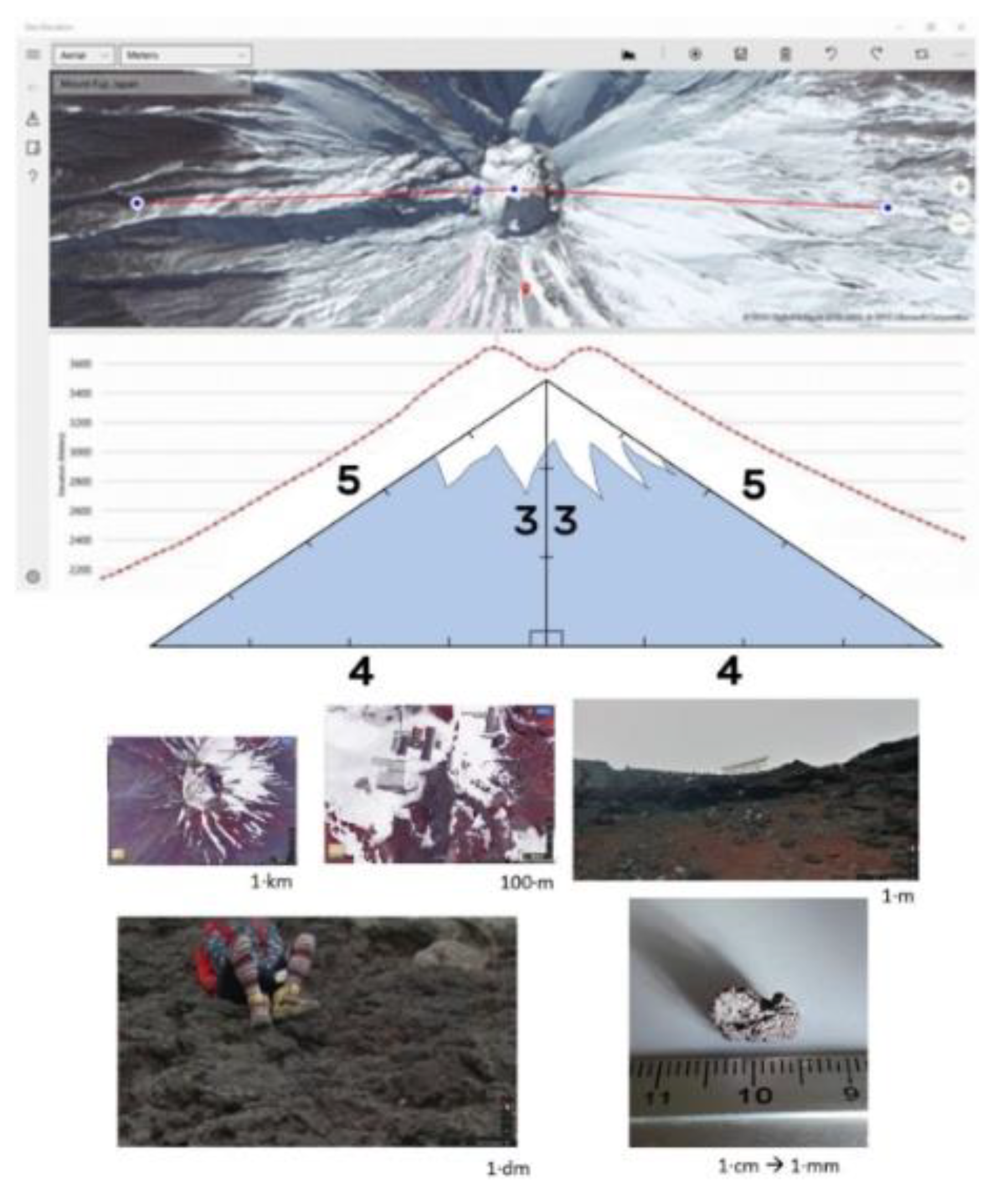
While raw global data is available (e.g., from UN-FAO’s “Global Terrain Slope and Aspect Data”), this is uncompiled, so an estimate of global slope is extracted from 30 arc-second resolution (ca. 1-km) summary data (Nunn & Puga 2004: appendix) [11] with mean slope for all 234 nation and dependent states (excluding Antarctica) here calculated as 3.94% or nearly 4% (ca. 2.29°). A 4% slope is 4 cm rise per metre run with the hypotenuse just 100.08 cm, or an extra 0.08% length, which is also an extra 0.08% area. Considering each country’s area and slope separately about doubles this to an extra 0.154% land overall (as calculated in attached data file), but this is still unrealistic.

A recent 2007 calculation from USGS’s Global Slope Dataset (pubs.usgs.gov/of/2007/1188/pdf/OF07-1188_508.pdf) of “accurate summary statistics at 30-arc-seconds describing the underlying 3-arc-second data” fails to yield a summary. An earlier paper [52] at five arc-minutes (10-km) had much lower global terrestrial slope of between 0–1.5°, whereas a later paper [51] shows that such high scales widely underestimate the true situation. Since land surfaces at 1-km scales are quite unrepresentative, so published terrain data at lesser scales are presented and reviewed in the succeeding sections.

3.1.1. Macro: Terrain

Recently, Ying et al. (2014) [51] claimed the first comprehensive estimate of the contributions of topography to the surface-area of the whole of China using Incremental Area Coefficients (IACs) as the percentage area increase of the surface area when compared with the projected area. This metric is the same as a tortuosity index. They highlighted scale-related factors and some potential environmental revisions of natural resources and ecosystem functions when area needs are taken into account. For China at 30-m resolution and a vertical error of less than 20-m, they calculated a mean surface area increase of 4.6% with the largest increment for a 50 km × 50 km cell being >45%. At 100-m resolution, the mean increase was 3.76%; at 1000-m (1-km) it was 0.5%; while at 10,000-m it was negligible (0%). Extrapolating these values linearly would give more than 4.5% increase in surface area at the 1-m scale (attached Excel chart). But, they also clearly showed (their figs. 5 and 9) that the results are exponentially dependent upon scale of observation: as resolutions approach the 1-m scale the area estimates increase markedly indicating threshold values for different classes of landscape below which the surface-area increment caused by topographic relief cannot be ignored.

Ying et al. [51] also found that the mean slope of the DEM across China at the spatial resolution of 30-m was 10.92° (19.29% slope), at 100-m it was about 9° (15.84%), while at 1000-m it was reduced to 3.53° (6.17%), and at 10,000-m it too was negligible; extrapolating this linearly would give about 12° (21% slope) at a 1-m scale for China. This compares to Nunn & Puga [11] data that, at the horizontal scale of 30 arc-seconds (926-m), have a mean slope of China of 5.49% (3.14°) just lower than Ying et al.’s 1000-m value and 3.8 times lower than the estimated 1-m value. It may thus be concluded that Nunn & Puga’s values are at least four times underestimations of likely 1-m scale values. Nunn & Puga’s overall Global average land area increase, based on slope at 1000-m resolution, was recalculated (Excel file attached) to be +0.154% of the flat area estimation, this multiplied four times to comply with an extrapolated 1-m scale from Ying et al.’s equivalence data, gives a value of around +0.616% overall globally. The following table summarizes these findings for China alone (

Table 3. Excel Recalculation for China Land Surface from Slope vs. Area [11,51].

Author	Scale m	Slope °	Slope %	Total Gha	% Diff.	% means *
Ying et al. (projected)	1	>12	~21	0.9574	>2.23	4.52
Ying et al.	10	11.65	20.62	0.9562	2.1	-
Ying et al.	30	10.92	19.29	0.9538	1.85	4.6
Ying et al.	100	9	15.84	0.9482	1.25	3.76
Nunn & Puga (data)	926	3.14	5.49	0.9378	0.15	-
Ying et al.	1000	3.53	6.19	0.9383	0.19	0.5
Ying et al. (flat land)	10,000	0	0	0.9365 **	0	0
% Diff. 1000 vs. 1-m		>240%	~240%	2.00%	>1074%	804%

* Apart from a 1-m projected value, other % means are as reported by Ying et al. (2014: figs. 5 and 9) [51]; it is not entirely clear why their % means vary to my % Difference recalculations using their stated formula. ** China’s flat area from Nunn & Puga [11] includes Taiwan, Hong Kong and Macao in order to agree with Ying et al.’s summary. Workings are attached in a Supplementary data file.

).

A real-world study of DEMs at finer scales is by Milevski & Milevska (2015: tab. 1) [53] (5–90-m resolutions) on a patch of ground (20 × 20 km = 400 km²) in the Skopje area of Macedonia. They found that slope accuracy increased 25 percentage points from a mean slope of 8.8° at 90-m to 11° at 5-m. This represents an increase in land area from its 400 km² base to 404.8 km² (+1.2%) and to 407.5 km² (+1.9%), respectively, with projection to >2% at 1-m resolution.

In the mountainous state of Himachal Pradesh in India, calculation by the local government [54] (tab. 3) gave 3-D TSA of 86,384.77 km² from original 2-D TMA of 55,342.79 km² or an increase of approximately 56.1%. However, resolution was at only 24-m or 71-m scale. At finer increment—say 1-m or less—the TSA can be expected to yield a much higher figure. Tentative, true surface areas from a study using 90-m SRTM DEM for the rugged states of Jammu and Kashmir [55] found 3-D and 2-D areas differed by nearly 25%: “(296,513 km² vs. 222,236 km², respectively)”. Finer slope resolution will considerably increase the surface reality to the planimetric model, and refined rugosity more so. Further real-world examples at the higher scale are needed.

Although more accurate datasets are increasingly available (e.g., eorc.jaxa.jp/ALOS/en/aw3d30/), it is expected that, as the resolution decreases from 30-m, the total land may easily double at each iteration, possibly approaching 100% at 1-m scale, i.e., double the land surface area to the map area. In support, a study using a 10 × 10 km plot in the mountainous Pyrenees (Nogués-Bravo & Araújo 2006: fig. 1) [56] has actual surface area of 280 km² or (180% greater area with ratio of 1:2.8) at 100-m scale; more than double that of 130 km² (30%) at the 500-m scale; while at the 1-km scale the surface area appears to be only about 110 km² (or just 10% larger).

In order to calculate the Soil Organic Carbon (SOC) in Chinese soils, Zhang et al. (2008) [57] calculated 3-D terrain for three mountainous states. The results increased soil surface area from 2-D of 78.04 Mha to 3-D area value of 84.02 Mha (7.7% increase although only at coarse scale of 90-m). From this, they calculated the SOC storage to 1 m depth increased from 10.9 to 11.9 Gt (+9.2%), which is of interest to a later section of this report.

Sutton & Lopez (2003) [58] “ironed out” Colorado finding it ~12% larger (at scale of 90-m).

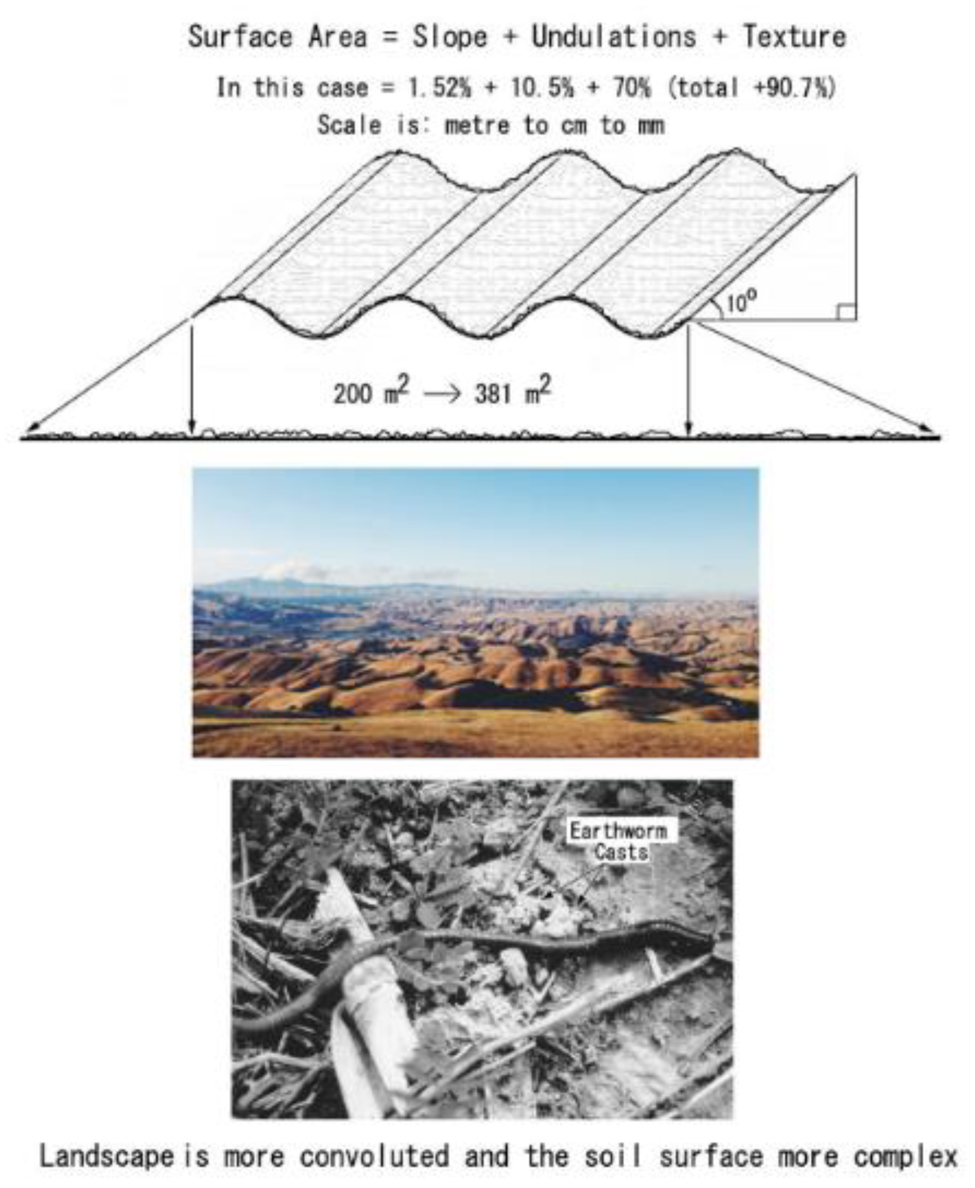
3.1.2. Meso: Tortuosity and Soil Roughness or Rugosity

The meso scale relates to an important measure of insolation defined as solar irradiance with energy measured in watt-hours per square metre (Wh/m²) or in the Langley, which is one calorie per square centimetre (= 41,840 Jm⁻²). These are both defined for horizontal area values and the latter cm² scale is approximately the same size as an earthworm burrow or surface cast. This is an appropriate level of observation for measuring basic ecological interactions locally and then extrapolating to a global value (as is routinely done by NASA, UN, FAO, IPCC, etc.). See also [38].

From the foregoing, it seems that tortuosity is strongly influenced by the observational factor: the more intense the scale, the higher the tortuosity index (T value). Indeed, a study in Canada by Martin et al. (2008) [59] shows a fourfold increase in bare earth tortuosity only when resolution was reduced to less than 10-cm starting from one metre scale. Martin (2008: fig. 5, tab. 1) [59] show a T_B value of 16 based upon a T_A Tortuosity index of 1.2 from a TSA of 240 m² and TMA of 200 m², i.e., 20% greater surface area for bare soil at their 0.75-cm scale. However, it appears this study, as with several others, did not adequately consider slope foreshortening, which for a straight hypotenuse of about 20 m and stated angle of 18 degrees gives a baseline of 19 m or 5% lesser base length. If we unrealistically assume that the slope is smooth and constant for its width, this then gives a simple Tortuosity Index of at least 240/190 = 1.26 (+26%), which is 5% above their calculation. Note that in this study [59] (fig. 5a), the vegetated rather than bare-soil hillslope had a tortuosity index of about 1.5 or a DSM area at least twice the bare earth DTM value.

A study from Brazil using a 3-D laser profile scanner at intervals of 1-cm (Bramorski et al. 2012: tab. 2) [60] reported soil tortuosity under conventional and no-tillage with mean index (T) values of 89.62 and 57.4 giving an overall mean index of 73.5 or +7250%! This tortuosity index was stated to be based on that of [61]. Communication with the author (Julieta Bramorski, email pers. comm. 11–18 July 2017) confirmed a mistake in their calculations and a new mean value of 1.33 (+33%) was arrived at. Yet, my re-working of the same data (kindly supplied by the primary author) gives a Tortuosity index (T_i) of around 4.56 that recalculated to allow for curved arc lengths rather than straight hypotenuses, gave a mean T_i of 7.16 (+616%). The constant ratio between these two means is 1.57 (+57%) and the combined mean of these two values gives a compromise of T_i = 3.6 (or +260%). The source data and Excel calculations are attached (“Julieta” section of Excel spreadsheet data file).

The mean for all four independent calculations at the mm scale is +94.0%.

3.1.3. Micro: Biodiversity, Productivity and Respiration

Of two German micro scale studies, one compares different methods of measurement but provides no usable data [62] (fig. A1); another [63] (tab. 2) has mean field index value of 1.23 (i.e., +23%) at 2 or 3-mm grid spacing with height accuracy better than 0.5 mm. A French study at 90 × 90-mm had a mean tortuosity index of around 2, i.e., double relief length to same projected length or +100% (Mirazai et al. 2008: fig. 6) [64]. Also, in Europe, (Tarolli et al. 2017: tab. 1; fig. 6) [44] summarized the various Roughness Indices and showed tortuosity doubling or quadrupling logarithmically when scale reduces from 40-mm to 4-mm scale with mean field index around 0.35 (a slight mistake in the legend is index “T_A” while text has “T_P”), this translates as an increase of 35% or 1.35 from their formulae (in their tab. 1) at this finest scale.

While defining Tortuosity-index as the ratio of total surface area to the map area i.e., T_B = TSA/TMA after Helming et al. (1992) [63], an Austrian report (Grims et al. 2014: tab. 3) [65] at 1-mm resolution has a field value mean of T_B = 2.63 that implies a true surface area more than two and a half times the flat horizontal footprint (i.e., +163%). [Mislabelled as “TB (%)” in Grims et al. (2014: tab. 3) [65], the primary author confirmed by email (pers. comm. 27 July 2017) that this is in fact the dimensionless index value not percentage]. Incidentally, this paper also measured soil organic carbon (SOC) and reported a mean value of 2.0% humus (= SOM or SOC?) in the study fields.

An online accessible but possibly unpublished Canadian thesis has cultivated soil surface area up to almost double the flat area (1.9 m/m²) with a mean value of laser roughness at the less than 1-mm scale of 1.6 (+60%) (Koiter 2008: sects. 2.3, 2.6, 2.7) [66].

The mean value for all five mm scale results is +108.2%.

3.1.4. Sub-Micro: SOM Surface Areas and Gaseous Exchanges

At the microporous scale, soil organic matter (SOM) and its colloids are reported to have adsorbic surface area for gaseous exchange of CO₂ of between 94−174 m² g⁻¹ (de Jonge 1996: tab. 2) [67] with a mean of 130 m² g⁻¹ (this value of 130 m² g⁻¹ is used in calculations of humic SOM bulk densities below and in an attached summary report). His paper quoted earlier studies showing SOM surface areas up to 800 m² g⁻¹, or six times greater, and this latter value approaches that of mineral zeolite or montmorillonite (also known as bentonite) clay. However, other studies only found 1 m² g⁻¹ [68]. The SOM data are on an “ash free basis”, i.e., just the dry, organic content of the sample is calculated even though a non-porous, inert mineral component was present in the samples. The solid phase densities average about 1.1 g cm⁻³ (de Jonge 1996: tab. 2) [67], and, regardless of whether from square or cylindrical measurements, the base area would be about 1 cm². The ratio of surface area (130 m²) to flat area (1 cm²) is thus approximately (10,000 × 130 =) 1.3 million times. 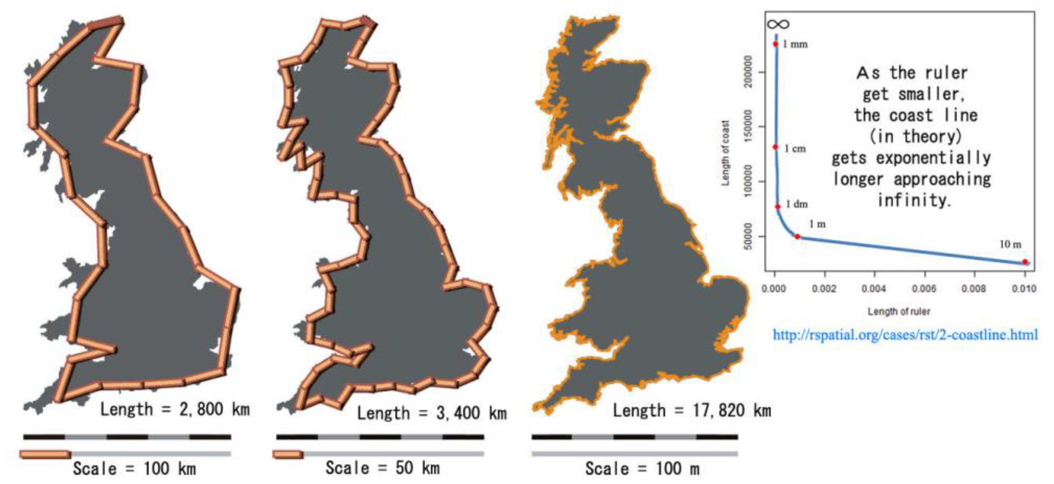As soil on a ‘flat-Earth’ occupies ~12 Gha then this would theoretically have surface area increase by 12 × (1.3 × 10⁶) = 15.6 Pha. This implies that true absorbic surface area of soil exposed to the atmosphere is almost infinitely expandable—as with the coastal paradox cited in Appendix A and as for the theoretical DTM and DSM models newly re-calculated in a section below.

3.1.5. Total Recalibration for New Land Surface Areas

Mean values from the studies reported above are tabulated in summary (

Table 4. Coarse Surface Topography and More Refined Roughness Indices (+% Areas).

#	Scale	Level	Area +%	Hilly	Author(s)	Applications
-	km	>1	0	-	NASA/NOAA	Astronomy
-	km	>1	0	-	Ying et al. 2014
1	m	1	4.5	No	Ying et al. (projected)	Terrain
2	m	1	2	?	Milevski & Milevska (proj.)
3	m	1	0.6	No	Nunn & Puga (recalculated)
4	m	5	1.9	?	Milevski & Milevska
5	m	30	4.6	No	Ying et al.
6	m	24–71	56.1	Yes	Anon.
7	m	90	25	Yes	Rashid
8	m	90	12	Yes	Sutton & Lopez
9	m	90	7.7	Yes	Zhang et al.
10	m	90	1.2	?	Milevski & Milevska
11	m	100	180	Yes	Nogués-Bravo & Araújo
12	m	100	3.8	No	Ying et al.
13	m	500	30	Yes	Nogués-Bravo & Araújo
14	m	926	0.2	No	Nunn & Puga
15	m	1000	10	Yes	Nogués-Bravo & Araújo
16	m	1000	0.5	No	Ying et al.
0	dm	-	-	-	-
1	cm	1	26	-	Martin et al. (recalc.)	Productivity, biomass
2	cm	1	33	-	Bramorski et al.
3	cm	1	57	-	Bramorski et al. (recalc.)
4	cm	1	260	-	Bramorski et al. (recalc.)
1	mm	1	163	-	Grims	Soil moisture/porosity,
2	mm	1	60	-	Koiter
3	mm	3	23	-	Helming et al.
4	mm	4	35	-	Kamphorst et al.
5	mm	90	100	-	Mirazai et al.
-	µm – nm	1	Millions %	-	Various	Microbiology, SOM/colloid gas exchange

).

In summary, the table above confirms km scale readings are unrepresentative. The three 1-m scale projections give mean +2.38% area, while the mean of all 16 macro scale readings is +21.25%, this latter possibly being the most applicable to more hilly terrains. For the meso cm-scale, the mean of all four results is +94.0%, while the five micro mm-scale results give mean of +108.2%. Thus, to a basic flat land area of 15 Gha we may apply between 2.4–21.3% increase, and, to 80% of this product (equivalent to a flat 12 Gha of soil), the other two progressive increases may be overlain. Finally, the approximately 20% (ca. 3 Gha) non-soil area initially subtracted, should be added to give a new total land surface, as it is calculated in the contingency summary (

Table 5. Summary Options of the Terrain/Relief Results for New Total Land Surface Area.

Condition	Area Increase for Terrain, Tortuosity and Relief, Gha				% Diff.	× Inc.
	(A) mean 1-m (n = 3)	(B) mean >1-m (n = 16)	(C) mean cm (n = 4)	(D) mean mm (n = 5)
% increase	2.40%	21.30%	94.00%	108.20%
(a) Land 15 Gha	15.4	18.2
(b) Soil 80% Gha	12.3	14.6
(c) Diff. (a–b) Gha	3.1	3.6
(d) Soil 12.3 Gha (Ab) × (C) then (D)			23.9	49.7
(e) Soil 14.6 Gha (Bb) × (C) then (D)			28.3	59
TOTAL (dD) + Difference (cA)				52.8 Gha *	252%	×3.5
TOTAL (eD) + Difference (cB)				62.6 Gha *	317%	×4.2

* Land total is between 52.8–62.6 Gha + 36 Gha ocean = 88.8–98.6 Gha for Earth’s new total surface.

).

Antarctica and Greenland include sub-ice terrain thus 15 Gha is the base value upon which macro tortuosity indices are imposed. Then, for soil-bearing land only or about 80% of outcome area (12.3–14.6 Gha), a median land increase is of ((×3.5 + 4.2)/2) = × 3.85, which is nearly four times original 15 Gha land. Combined with an immutable flat ocean area of 36 Gha, the new land area of 53–63 Gha gives a new World area of 89–99 Gha, albeit superimposed upon this is a theoretically infinite SOM microporosity. As to which set of scales is selected, this depends upon what practical calculations (e.g., biomass, NPP, gas exchange, proper allocation of grant funds, etc.) are deemed most relevant for a particular study. A Fermi calculation (below) allows area increase to ~100 Gha.

3.2. Theoretical DTM Model and Fermi Calculations

Jenness (2008) [47] noted slope-aspect algorithms generated indices around 1.6–2.0 (as per Hodgson 1995 [48]) with a median 1.8. Thus, from a land surface of 15 Gha, at the metre or dm scale, this may increase to 27 Gha, and, as ~80% supports soil, its tortuosity at the cm scale may be similarly increased by 1.8 times (27 × 0.8 × 1.8 =) 38.9 Gha. It is possible to argue that the mm scale allows a further 1.8 times area to give a final total of (38.9 × 1.8 =) 69.98 or about 70 Gha. This plus 36 Gha ocean and 5.4 Gha barren land (27 × 20%) gives a theoretical new total surface area of ~111.4 Gha, which is tolerably close to the values (around 100 Gha) that were calculated above from on-the-ground field readings.

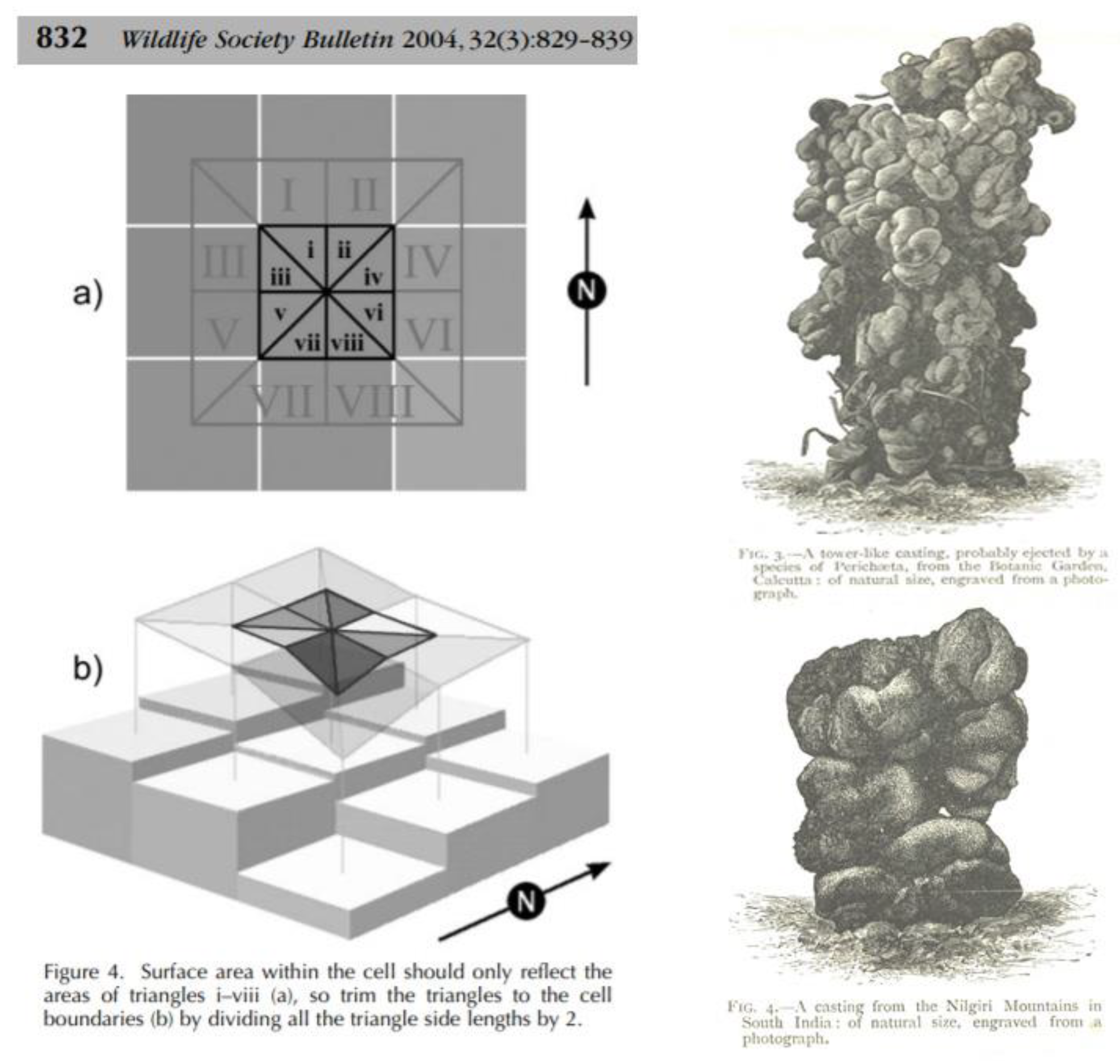
In support of higher land area, a study from Germany [69] discusses the problems, technical issues, and recent developments whilst providing examples from model terrains seemingly at 1-m resolution at least for test square mapped landscapes with perimeters of 400 m (but 2-D area of just ca. 1000 m² or 31.3 m side or perimeter of 126.5 m in their fig. 4?) derived from their fig. 2 of square patch areas (after Jenness 2004 [47]). Increases of patch areas show in their fig. 4 are from 2-D of about 1000 m² to 3-D of up to 10,000 m² or 20,000 m², i.e., by ten or twenty-fold (or 900–1900%). Their (fig. 4) “Average Surface Roughness” indices go from an obvious zero in 2-D up to eight in 3-D, or by an infinite amount but implied as an eightfold area increase (+700%). This gives further support for current fourfold landscape increase (from 15 → ca. 60 Gha or +300%) as being entirely reasonable if not a wide theoretical underestimation of total land area.

Because the true surface of the land is paradoxical and it depends upon arbitrary, shifting, and overlaid scales of observation, the most pragmatic solution is perhaps to accept a compromise Fermi value pending further acuity. To transpose the scale problem it may be more practicable to arrive at a reasonable and ‘convenient’ working model of global surface area (i.e., the surface directly exposed to sunlight, atmospheric gas exchange and rainfall) as 100 Gha with 64 Gha attributed to landscapes and topsoils.

DTM for DSM Recalculations

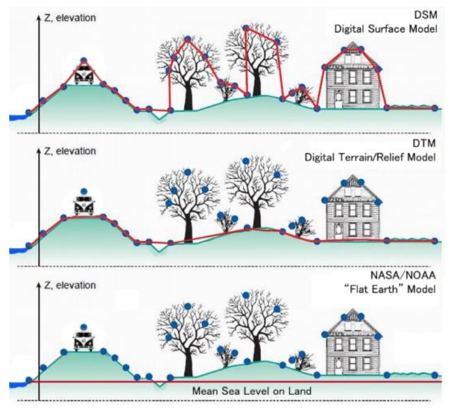
Overlain upon the bare-earth terrain DTM is an increasing superficial DSM (cf. Figure 6). An estimate of effective DSM is possible if we apply the Leaf-Area-Index (LAI). This dimensionless quantity characterizes effective plant cover defined as the one-sided green leaf area perpendicular to flat unit ground surface area (LAI = leaf area/flat ground area, m²/m²). LAI ranges from 0 (bare ground) to ~18 (dense forest canopies) and a global average (from Asner et al. 2003) [70] is 4.5. These authors state “LAI is a key variable for regional and global models of biosphere-atmosphere exchanges of energy, carbon dioxide, water vapour, and other materials”. It is surely just as important to have estimates of a global DTM and DSM too. Prof. Greg Asner (pers. comm. email 20 July 2017) kindly clarified: “That estimate is the average of studies published for different vegetated ecosystems, so it does not represent the actual global land area”. Thus only soil bearing terrain is considered in the following calculations.

As about 80% of land supports soil, on the conventional flat-Earth view and in the new view, a rough estimate of prior, conventional, DSM is of 12 Gha × 4.5 = 54 plus 3 Gha ice or desert-covered land = 57 Gha. From my new topographical calculation DSM is (64 Gha × 80% =) 51 Gha soil × 4.5 LAI = 230 Gha, which is an important measure related to global photosynthesis potential (plus a lesser ocean contribution). Since LAI is for one side of the leaf, then the total for both sides of a leaf presumably gives 230 × 2 = 460 Gha DSM plus 3 Gha non-soil land, plus 36 Gha from flat oceans = 499 Gha global DSM estimate. Cities or townscapes occupy about 1–3% of land area with additional parks, gardens, verges, etc. that would add slightly to this very rough estimate of DSM. Moreover, this may be an underestimation, as, rather than a LAI of 4.5, Whitman et al. (1998: 6580) [23] assumed a more than double LAI of 10 (but source and whether single-sided were unstated).

Microporosity will futher increase the DSM since, strictly, any internal surfaces or pore spaces are also part of the surface area if defined as the interface of solids or liquids exposed to air. Just considering plant respiration, this internal areas of stomata of leaves is possibly unquantifiable. However, leaves are a major contributor to humic soil organic matter (SOM) with its micro-porous surface area for gas exchange shown as between 1.5–120 Pha and an argument may be made that this is the truly astronomical surface area of land making the mere quadrupling of the DTM of ‘flat-Earth’ area of just 15 Gha to 64 Gha seem entirely reasonable and easily justified, as indeed is the almost ten times increase of coarse DSM from 57 Gha to 499 Gha.

Subterranea (e.g., caves, caverns, or karsts) are an additional but minor ‘surface’ area consideration, but earthworm burrows may be considerable. Burrows systems, as noted above, were found to extend for up to 888 m/m² in length (=8880 km ha⁻¹) and their void volume varied tenfold from 1.3–12.0 m²/m² ground surface in the upper 1.2 m of soil during an observation period of 1.5 years (Lee 1985: pp. 196, 208) [29,49]. On conventional 12 Gha flat soil, this is at least 1.3 ha/ha × 12 Gha = 15.6 Gha. However, on rugose topsoil, this would be about four times greater, i.e., at least 62.4 Gha that may vary up to 624 Gha or a 0.6 Tera-hectare volume of below-ground earthworm burrow voids. It should be noted that that study mainly represented pasture soils in France, but the samples excluded both the 0–6 cm layer of soil and also burrows <2 mm in diameter (Lee 1985: 196) [29]. Including these smaller burrows and other micro pore spaces, in the topsoil especially, would presumably increase underground volumes of sub-surface spaces substantially. Nevertheless, including sub-soil voids may double the DSM to (499 + 624 =) 1123 Gha or 1.1 Tera-hectare. The flat ocean’s surface (that exposed to Sun, air, rain) remains at 36 Gha and its bathymetry or rugosity largely an irrelevancy.

3.3. Bulk Density (BD) Backcheck

Support for the current terrain argument is from bulk density (BD) that compels revision. Tangible sub-samples are taken on the ground at fixed core sample volumes with a constant planimetric area (cm⁻² or m⁻² perpendicular to the centre of the Earth) and then multiplied by a biome’s area, thus mass may be adjusted to comply only by adding biome area by adding terrain/topsoil relief.

For habitable biomes supposedly totaling 12.3 (flat) Gha, (Whitman et al. 1998: tab. 2) [23] gave mean soil bulk density as 1.3 g cm⁻³ (= tm⁻³) and (Lee 1985: 195) [29] assumed a bulk density of 1.4 g cm⁻³, so a reasonable mean may be 1.35 g cm⁻³. Total SOC to one metre recalculated (from FAO’s Harmonized World Soil Database, HWSD, as noted in attached Supplementary data file) gives median values for SOC of around 1.3% and their mean soil BD is ~1.4 g cm⁻³ (close to 1.35 g cm⁻³). Total conventional ‘flat-Earth’ topsoil mass to 1 m depth would then be [(123 × 10¹² m³) × 1.35 tm⁻³ = 166 × 10¹² t =] 166,000 Gt topsoil and 1.3% SOC = 2158 Gt C.

Allowing for organic soils having lower BD than mineral soils, highly organic, peaty Histosol humic-SOM BD is 0.1 g cm⁻³ (Köchy et al. 2015: 354) [71] as an ideal for SOM organic matter with 50% C (from Pribyl 2010) [72]. Prior best estimate of total SOC to 1 m depth (e.g., by IPCC 2013, www.4p1000.org, etc.) was 1500 Gt giving total × 2 SOM of 3000 Gt on planimetric 12 Gha land or 120,000 m³ to 1 m depth. Thus, a BD was of (3000/120,000 GtGm⁻³ =) 0.025 g cm⁻³, which is below the required SOM BD of 0.1 g cm⁻³ and thus needs × 4 mass. The only plausible way to increase mass is by increasing real biome area to allow for terrain/topsoil. When the soil surface is doubled for terrain and again for topsoil micro-relief then mass of soil increases. Since BD measurements typically use a core cylinder of fixed volume, thus the actual undulating surface area is immaterial. For demonstrative purposes of real BD, if we assume quadruple SOM 3000 Gt → 12,000 Gt whilst maintaining 12 Gha planimetric area (or rather its volumetric equivalent to 1 m depth), the resulting bulk density of 0.1 tm⁻³ exactly matches the required mean of 0.1 tm⁻³ (Q.E.D.).

Is it reasonable to increase land area values fourfold? Given a BD mean of 1.35 g cm⁻³ (or tm⁻³) and allowing for a fourfold increase in soil occupied land area (i.e., 12 Gha × 4 = 48 Gha), then total soil mass to 1 m would be (480,000 Gm⁻³ × 1.35 t) = 648,000 Gt globally. If SOC is 1.3%, then the total SOC to 1 m is 8424 Gt (that tolerably agrees with a 8580 Gt value calculated below from empirical sources).

Similarly, a planimetric soil area of 12 Gha to 3 m depth (= 360,000 Gm³) requires a new SOM of 36,000 Gt to give the required 0.1 g cm⁻³. If 3 m SOC doubles from 8580 → 17,160 × 2 = 34,320 Gt SOM giving BD of (34,320/360,000 =) 0.095 tm⁻³ or tolerably 0.1 g cm⁻³ (Q.E.D.). However, both mean bulk density and SOC % are perhaps less reliable at depths greater than 1 m.

Another calculation, possibly artifactual, is with prior SOC >1 m depth (Köchy et al. 2015) [71] of 3000 Gt × 2 for 6000 Gt SOM on planimetric 12 Gha if to a sample depth of, say, 3 m = 360,000 Gm³ giving real SOM bulk density of just 0.016 tm⁻³ or out by a factor of six for average BD of peaty SOM of around 0.1 tm⁻³. This discrepancy may be resolved with reference to terrain/relief by about ×6 from flat 12 Gha to about 72 Gha that, plus 3 Gha hot or ice deserts and 36 ocean, gives total area of 111 Gha. Seeming slightly excessive this may be ultimately reasonable and is, coincidentally, nearly the same value of 111.4 Gha as arrived at earlier with theoretical DTM models.

Reasoned indications thus point to Earth’s real surface area in the realm of 111 Gha with 75 Gha bare-earth (68%) and just 36 Gha sea (32%) or about two-thirds of the World being land-based.

Standard BD reference of planimetric 12 Gha to the centre of the Earth, overlain by terrain/soil relief, etc. by using multiplication factors are summarized, assuming the global mean BD 1.35 gm⁻³ and SOC 1.3%, as compared to current conventional SOC values (of 1500 Gt to 1 m or 3000 Gt to 3 m depth), showing their multiplication shortfalls (

Table 6. Contingency Factors from Mean Bulk Density (BD) with Soil Organic Carbon (SOC) Mass.

BD tm−3	Area Gm2	Factor	Soil Gt	Depth m	SOC @ 1.3% Gt	cf. SOC Gt *
1.35	120,000	×1	162,000	1	2106	×1.4 (cf. 1500 Gt)
1.35	240,000	×2	324,000	1	4212	×2.8 (cf. 1500 Gt)
1.35	480,000	×4 **	648,000	1	8424	×5.6 (cf. 1500 Gt)
1.35	720,000	×2	972,000	3	12,636	×4.2 (cf. 3000 Gt)
1.35	720,000	×4	1,944,000	3	25,272	×8.4 (cf. 3000 Gt)

* Multiplication factors required on current IPCC SOC values to produce indicated SOC @ 1.3% total. ** Quadrupled land or soil relief area is most likely and reasoned situation, as explained in the text.

).

This table shows IPCC’s current conventional 1 m SOC estimates (ca. 1500 Gt) is out by a factor of 1.4, and other possible terrain scenarios by between 2.8–8.4 times. Terrain × factors are for coarse landforms, and also for superficial cm² + mm² relief details that, at both these finer scales, are mainly composed of superficial SOM-humus/earthworm casts.

For reference (from Wikipedia), amorphous carbon densities are 1.8–2.1 g cm⁻³ differing from dry soil bulk density that varies in its minerals, biotic, as well as its air space voids (porosity).

Although clearly revealing conventional underestimations of SOC/SOM, these variable result from BD calculations probably relate to difficulties in obtaining global BD means and their complexity with soil depth. The upper 1 m results are likely most reliable. Full calculations and justification for bulk density assay may be scrutinized in the attached Supplementary Files.

3.4. Soil, C and a “Missing Sink” Discrepancy

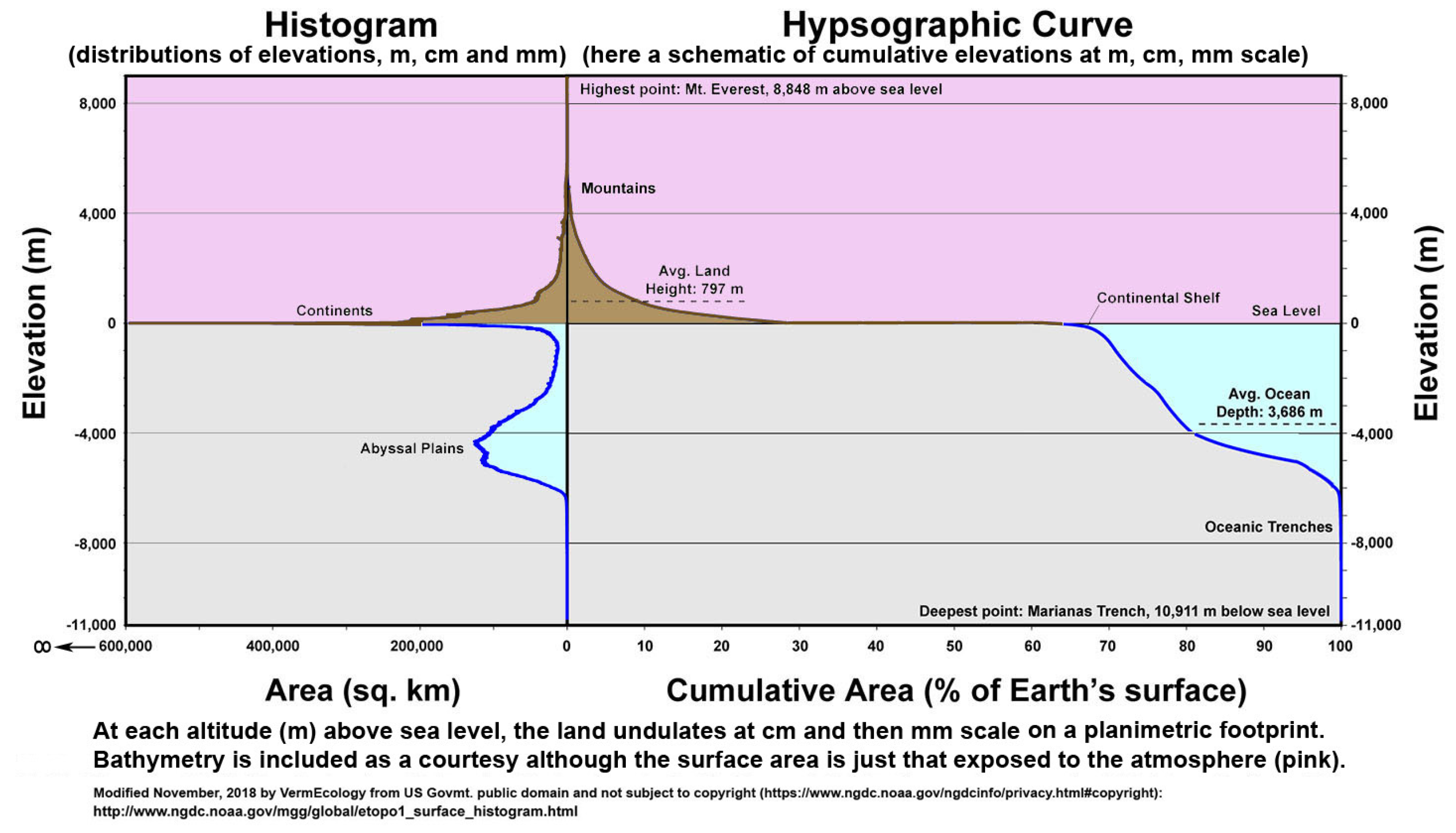
Primary sources of global carbon budgets as used by IPCC (e.g., by authors such as Batjes, Haughton, Jackson & Jobbágy, and Prof. Rattan Lal) invariably give a land area total of about 15 Gha on a globe of around 51 Gha; however, this is for an idealized flat surface whereas it is self-evident that land is hilly (cf. Figure 1). With topological consideration, all land areas may be slightly increased at one kilometre scale (by ~1–5%). As already noted above, on study showed topsoil surface area from 2-D to 3-D increased by 7.7% at a coarse scale of 90-m and its SOC storage to 1 m depth was upped by +9.2% [57]. Also, as calculated above, 1-m scale projections give mean land increases of +2.38–21.25% (median about 10%), and soil carbon may certainly be increased, likely doubled or quadrupled, at finer resolutions. Factors are: sub-surface SOC, roots, and soil biota. Justification is that these are measured at the mm to cm scale and then applied at the m to km scale.

Lal (2008: fig. 1) [73] cites a “missing sink” of 2.6 Gt/yr C, as discussed in a Supplementary file.

3.4.1. Total Soil Carbon (SOC/SOM) for Recalculation of Global Carbon Budget

Relating to global warming and Greenhouse Gasses (GHGs), carbon is by far the major issue with the problem, and the solution, to be found mainly in the ground (

Table 7. Global Warming Potential (GWP) of Gasses from Duursma & Boisson (1994: Table A3) [4] *.

Greenhouse Gas GHG	Potentiality (GWP)	Emission (1990) Gt	Contribution %
CO2 carbon dioxide	1	26	61
CH4 methane	21	0.3	15
N2O nitrous oxide	290	0.06	4
CFCs fluorocarbons	1000s	0.007	9
HCFCs fluorocarbons	1000s	0.001	0.4
Others			10.6

* Note: these rates were later revised somewhat by IPCC.

, Figure 10).

Global SOM-humus stock data are not readily available but they may be calculated from global soil organic carbon (SOC) given as 1500 Gt by IPCC 2013, www.4p1000.org 2015, http://www.fao.org/3/a-i6937e.pdf 2017, see [74] (fig 1), 2300 [41], 2397 [75], or as 2956.5 that is quoted as ~3000 Gt [71]. Value differences are largely due to depth of topsoil sampling [8,74], the first is 0–1 m, the second is 0–3 m, and the third and fourth most recent values include soil greater than 1 m [71] (by Köchy et al. 2015 who possibly have mean 4.0 m for peats or to depth of soil for other types?). Then, taking their higher value of 3000 Gt and applying the revised van Bemmelen factor of SOM = 2 × SOC (Pribyl 2010) [72], the total SOM is 6000 Gt on a dry-weight or an “ash free basis”. However, all values are for ‘flat-Earth’ calculations of just ~12 Gha soil area having a SOM bulk density (BD) of 6000/120,000 = 0.05 tm⁻³, and if this is doubled for terrain and coarse relief, then the total topsoil mass is presumably increased too. That is, for SOC from 3000 → 6000 Gt and for SOM humus 6000 → 12,000 Gt with a new SOM bulk density, keeping same area due to fixed core sample volumes, as 12,000/120,000 = 0.1 tm⁻³ the significance of which is already noted in the BD section above. These new increased values, however, may themselves be underestimations.

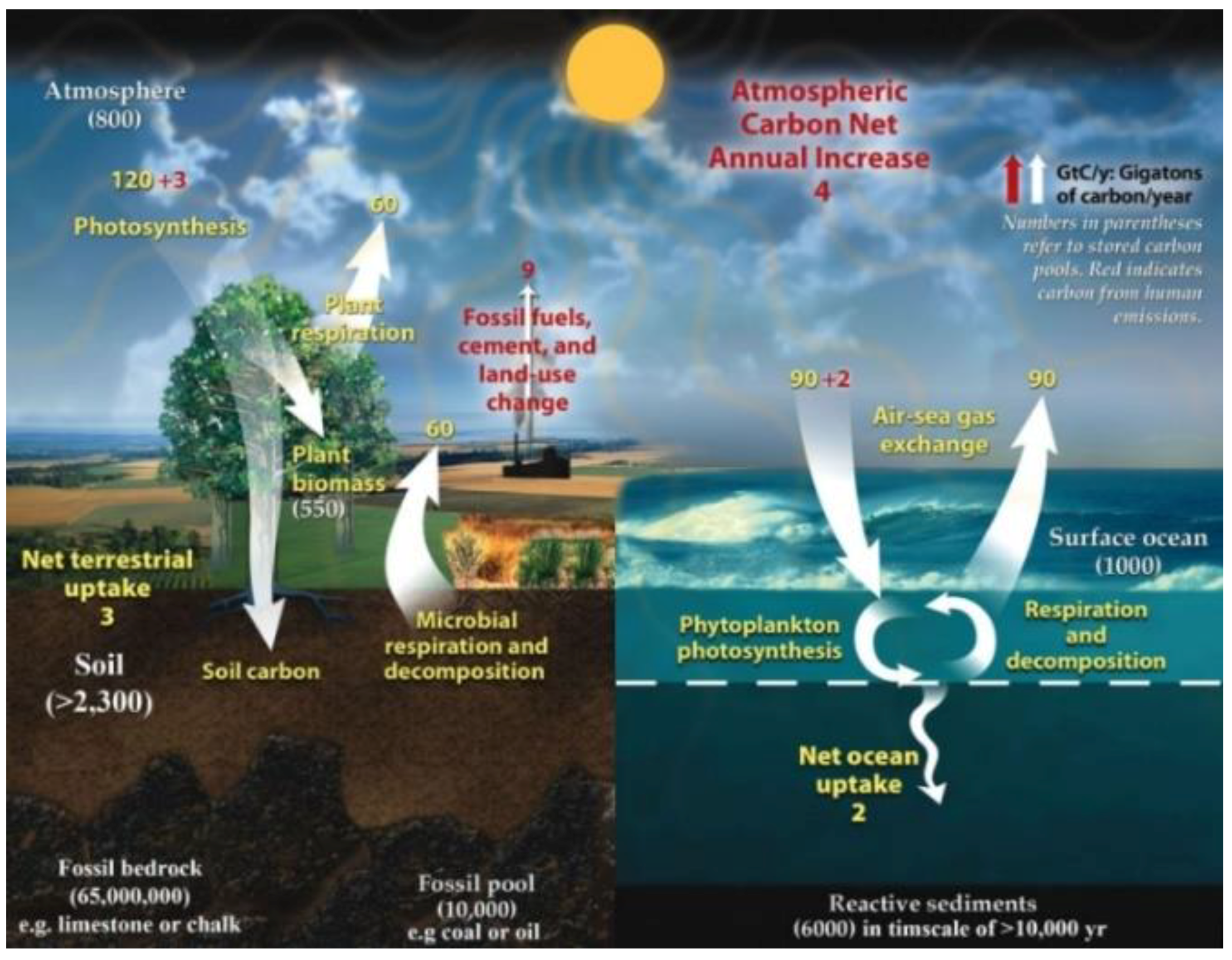
In addition to terrain considerations, [74] (p. 11) noted that: “Soil carbon values require allowance for intractable glomalin adding a further 5–27% to almost all SOC tallies (Comis, 2002). Plus data from deep soils may increase budgets: e.g., Harper & Tibbett (2013) found C up to five times greater in Australian soils at depth >1 m and down to 35 m in some cases. The Walkley-Black method itself underestimates total C by about 20% with a correction factor of ca. 1.3 often required [this W-B correction is from Pribyl, 2010], whereas latest techniques using mid-infrared (MIR) spectroscopy give more accurate readings. These three factors combined would surely increase soil SOC totals”.

Thus, assuming that soil depth factors are already included with terrain area, 6000 Gt SOC × 1.3 W-B correction = 7800 Gt plus, say, median value 10% for glomalin = 8580 Gt total soil carbon. Worldwide, the reactive organic carbon stored in soils (herein from 3000 → 8580 Gt) greatly exceeds the most generous amounts that are attributed in above-ground phytomass (700 Gt), plus atmosphere (800 Gt) and surface oceans (1000 Gt), which equal just 2500 Gt in total when combined (cf. Figure 10).

Global topsoil humic SOM is then also raised from 8580 SOC × 2 to approximately 17,160 Gt (but, as calculated above, to greater than 1 m depth this may be doubled again to ~34,320 Gt).

Turnover time for fast pool carbon is estimated at 23 yrs [75] cf. 10–15 yrs according to (IPCC 2007) [76]. These then would also be duration for processing of humic SOM by detritivore earthworms, as indeed Darwin (1881) [31] extrapolated from his minute observations: “All the fertile areas of this planet have at least once passed through the bodies of earthworms”. From this, it was reasoned [74] that all atmospheric carbon is theoretically processed via leaf-litter through the intestines of earthworms in ~12-year cycles. That is, unless populations are severely depleted [15].

3.4.2. Root Stocks, Vesicular-Arbuscular Mycorrhiza (VAM) Hyphae, Litter, Crusts, and Earthworms

Relating to above-ground vegetation are the often ignored underground root-area-indices (RAIs) with fine roots a prominent sink for carbon, often much greater than that of vegetation above ground. Extending many metres below ground, interlinking with kilometers of symbiotic VAM fungal hyphae, roots are routinely excluded from soil samples by manual removal and sieving.

Estimated total root biomass was 292 Gt containing 146 Gt carbon and representing 33% of total annual net primary productivity (Jackson et al. 1997: tabs. 2–3) [37]; however, this seemingly was updated by Mokany et al. (2005: 95) [77] to 241 Gt C for roots. UNEP (2002: 10) [26] estimate that probably over 80% of plant production enters the soil system either through plant roots or as leaf-litter. It was also shown that perhaps 50% of below-ground allocation is released as extra-root carbon exudates [78], some being ‘traded’ with microbes for Nitrogen fixation or other growth factors. Additionally, estimates are of at least 15 Gt C for soil mycorrhizal VAM hyphae [79].

Some vegetation surveys, but certainly not all, make allowance for below ground biota and for living or dormant biomass and dead necromass. Also, generally excluded from calculations of SOC (and SOM) mass is leaf-litter—an important part of the soil profile transitioning to humus—that contributes considerably to the global carbon budget with a “pedologic pool” of 40–80 Gt giving a median stock value of 60 Gt (Lal 2008: fig. 1) [73,80]. Moreover, autotrophic biofilm or biocrust (e.g., bryophytic liverworts, hornworts, and mosses plus microfungi/yeasts, photosynthetic green algae, lichens, and Cyanobacteria or Cyanophyta) also coat and inhabit the convoluted superficial and interstitial surface rocks, topsoil, and sand. These ‘cryptogamic covers’ of biocrust total 5 Gt C [81].

Complete soil carbon thus strictly includes root mass (241 Gt), leaf-litter (60 Gt), plus VAM (15 Gt), biocrusts (5 Gt), and earthworms (2–4 Gt from [82]) to total 323 Gt that may all be reasonably doubled to allow for terrain to (323 × 2 =) ~650 Gt carbon. If this is then added to the 8580 SOC × 2 = 17,160 SOM calculation from above, it gives a new total SOM to depth of about 17,810 Gt (as per Abstract, but, as also estimated above, this may likely be doubled again to ~34,320 Gt).

3.4.3. Microbial Biotic Carbon: Living, Dormant or Dead (Including Fossils and Geology)

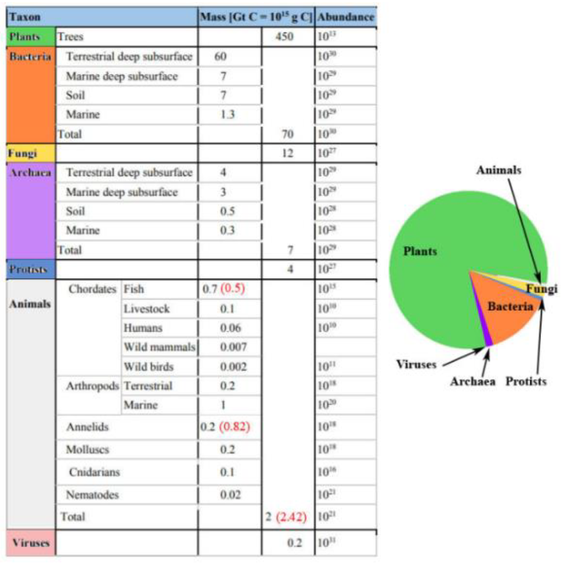
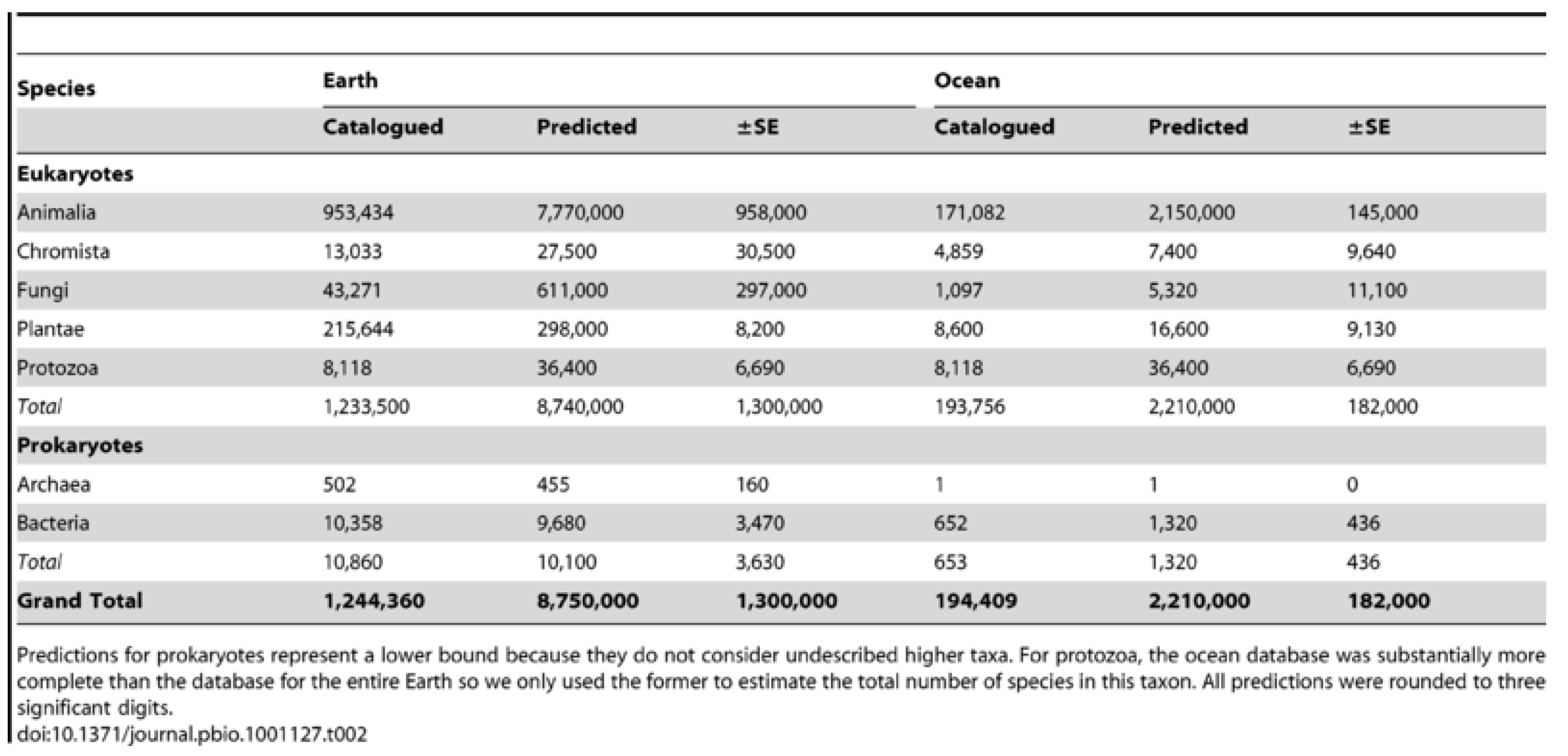
Regarding microbial biotic carbon (most of which is included in the SOC data), a much-cited study (Whitman et al. 1998: tabs. 2, 5) [23] of prokaryotes [viz. Monera (simple bacteria) and Archaea] estimated their total cellular carbon biomass as up to 450 Pg (= 450 Gt) that these authors stated to equal the carbon storage in land plants. Their allocation of prokaryotic mass was approximately 50:50 ocean to land (actually 48–241 Gt carbon in soil versus 305.2 in sea). But, their land estimates (tab. 2), although up to 8 m depth, is for ‘flat-Earth’ biome areas, which they say totals 12.3 Gha excluding ice, multiplied by numbers of microbe cells sampled from each biome; whereas, for ocean in (their tabs. 1 and 3) are unit volume of sea (cells/mL) thus immutable, or cells/cm³ in sediments at depths (most in 0.1–10 m depth). It is likely that terrain/relief will more than double the land count and thus the total biomass by at least one third. Taking their upper 241 Gt value × 2 for land terrain and ×2 for topsoil relief = 964 Gt (plus 305.2 Gt in sea = 1269.2 Gt total biotic carbon). However, a more recent ocean re-assessment [6] reduced microbial biomass on the seafloor due to paucity in actual deep ocean cores from their original 303 billion tonnes of C to just 4.1 billion tonnes representing just 0.6% of Earth’s total living biomass and reducing the total global biotic carbon to about [964 + (2.2 + 4.1) =] 970.3 Gt with most (i.e., 964 Gt) in soil. Thus, land’s C allocation (99.35%) is yet again greatly enhanced proportionately to that of the ocean (0.65%) (cf. Table 2, Figure 3).

The UNEP (2002: tab. 2.1) [26] “World Atlas of Biodiversity”, despite claiming global coverage, is mainly concerned with marine/ocean/water and barely mentioned soils, nevertheless, had total carbon content of Earth as ~100,000,000 Gt C, allocated as in the following, modified, and corrected, tables (

Table 8. Revised Reactive/Recyclable and Non-reactive (Stored) Carbon.

Global Carbon	Stored C Gt	Reactive (Biotic and Inorganic) C Gt
Sedimentary rock organic C	16,000,000
Sedimentary rock carbonate	65,000,000
Dissolved inorganic C in deep sea	38,000 *
Organic carbon in deep sea	1350 *
Reactive C in surface sea		500–1000 *
Organic carbon in soil (0–1 m)		8600 **
Atmospheric CO2—C		800
Biomass in + on land (plants + micro)		>2000 ***
Biomass in sea		<15 ***
TOTAL	81,039,350	>12,415

After UNEP (2002: tab. 2.1) [26]. Notes: * Sundquist & Visser (2003: fig. 1) [83] show only 900 Gt surface sea carbon is reactive in yearly to decade intervals, whereas most ocean carbon is un-reactive to the atmosphere for centuries, millennia or up to geological timescales. ** The soil carbon estimates, originally at 1500 Gt, are upped to 8580 Gt to allow for microbes + terrain, values at >1 m depth may double this to 17,160 Gt C. *** Originally 560 Gt mainly for above-ground plants, present land total accounts for roots (640 Gt) and sub-soil biota (964 Gt) both already doubled for terrain; sea biomass of “5–10” Gt is updated with values from Tables below.

and

Table 9. Tabulated Data Combined with for Total C & O_2.

Medium	Carbon C Gt (%)	Oxygen O2 Gt (%)
Air	6.4 × 102 (0.00%)	1.2 × 105 (99.2%)
Land (mainly in rocks)	8.1 × 107 (99.96%)	NA *
Sea	3.5 × 104 (0.04%)	9.8 × 103 (0.8%)
TOTAL	8.1 × 107 (100%)	1.21 × 105 (100% *)

After Duursma & Boisson (1994: tab. 2) [4]. * Oxygen in rocks is substantial but unknown; on average about 25% topsoil volume is aerated, lessening to the depth of working of earthworms (~15 m) [33]; but life occurs on land up to 19 km deep (e.g., www.astrobio.net/extreme-life/life-might-thrive-dozen-miles-beneath-earths-surface/).

).

3.4.4. Above and Below-Ground Biodiversity and Biomass Carbon Rechecked (plus Ocean C)

It is remarkable that almost always overlooked or undervalued in biodiversity assessments are the communities and networks of below-ground soil biota that represent both the Earth’s highest diversity and its greatest biomass (even without consideration of terrain effects) (Figure 11 and Figure 12).

Most calculations of terrestrial fauna and flora (microbes, plants, fungi and animals) based upon ‘flat-Earth’ biomes or habitats require revision and likely doubling or quadrupling, and this affects relative ocean proportions. Although the total animal biomass appears to be insignificant in comparison to land plants [26,81] just considering megadrile earthworms, recent calculations [82] of 1.3 quadrillion worms with fresh weight ‘vermi-mass’ of 4–8 Gt, may be doubled for terrain relief to 2.6 quadrillion and a massive 8–16 Gt (with carbon content up to 4 Gt). If correct, earthworms would be truly significant (as Darwin 1881 surmised), even though they are apparently annihilated under conventional, chemical agriculture [15,29]. When compared to a recent best estimate of global fish “wet weight” of just 1–2 Gt [85] (with carbon at most 0.5 Gt), this casts glib comments about worms being good fishing bait in a whole new light.

Life on Earth may be elevated as summarized in carbon calculations above. However, as noted, an ignored sub-surface biomass in the rhizosphere of VAM fungi and roots substantially increase the land proportion [37]. For roots Mokany et al. (2005: 95) [77] said: “Our results yield an estimated global root stock of 241 Pg C, a similar value to that proposed by Robinson (2004), but about 50% higher than the 160 Pg C estimated by Saugier et al. (2001). This dramatic increase in estimated global root carbon stock corresponds to a 12% increase in estimated total carbon stock of the worlds vegetation (from 652 to 733 Pg)”. Searching their sources, the value 652 Pg is likely above-ground vegetation (from “Saugier et al. 2001”) of 492 Pg, plus Robinson’s (2004) [78] estimate of 160 Pg root (492 + 160 = 652). The 733 is seemingly from the same above-ground value plus their own estimate of 241 Pg root carbon (492 + 241 = 733 Pg = Gt).

Thus, a total of above- and below-ground land vegetation are reasonably accepted as 733 Gt C, which, along with bacteria from Whitman et al. (1998: Table 5) [23] and as re-assessed by [6] of 241 Gt vs. 6.3 Gt in soil vs. sea, respectively, gives biomass carbon on land of (733 + 241 =) 974 Gt C. Mycorrhizal VAM-fungal hyphae and biocrusts add 15 and 5 Gt (974 + 20 = 994), plus 2–4 Gt earthworms [82] and 7 Gt for other organisms [81] = ~1000 Gt total. This terrestrial carbon may be doubled for terrain (and possibly doubled again for soil relief, especially for microbes) to give between 2000–4000 Gt land C, plus an ocean contribution of just 14.8 to total at least 2014.8 Gt of living, respiring, biotic carbon (

Table 10. Revised Global Biotic Carbon on and in the Soils on Land and in the Sea.

Biota	Soils Gt C	Sea Gt C
Plants above ground	492	-
Roots below ground	241	-
Bacteria	241	6.3
VAM hyphae + biocrusts	20	-
Earthworms	2–4	-
Fish *	-	0.5*
Other organisms **	7	8
TOTAL (%)	~1000 (98.6%)	14.8 (1.4%)
TOTAL × 2 for terrain (%) ***	~2000 (99.3%)	14.8 (0.7%)

* Global fish stocks confidently calculated as 0.89–2.05 Gt wet weight [85] of which just 0.15 Gt (<10%) is total annual combined fish catch plus aquaculture (en.wikipedia.org/wiki/World_fisheries_production) still the highest on record to date; fish total is ~0.5 Gt C. ** Other organisms from Bar-On et al. (2018) [81]. *** At least 2000 Gt of living biomass is terrestrial, that may be justifiably doubled yet again for soil relief, especially for smaller organisms.

).

As carbon is universally about 50% dry weight, a new value is at least (2000 × 2) = 4000 Gt dry biomass on land plus (14.8 × 2) = 29.6 Gt in sea. Since water content is taken as 50% [~30% in wood (www.wood-database.com/wood-articles/wood-and-moisture/) and 40–70% in bacteria [86,87] with median value ~50%], then this value is doubled again to at least 8000 Gt wet weight on land plus (14.8 × 4 =) ~60 Gt in sea to give new total for Earth’s living, respiring, fresh mass of ~8060 Gt, or roughly ~8 Tera-tonnes (Tt) of biomass.

These data compare to [88] Vaclav Smil’s (2011) total dry biomass of Life on Earth he estimated as just 1600 Gt (here more than doubled to at least 4029.6 Gt maybe 8060 Gt). As a cross-check, the total biosphere carbon is estimated at between one to four Trillion tons [89]; thus, my current estimate of around 2000 Gt C (2 Tt) is about mid-range but is closer to the best case scenario of 4 Tt.

Total terrestrial carbon of at least 2000 Gt in land organisms mostly intermixes with the 8580 Gt or so SOC in SOM or humus as active carbon stored and recycled on land, as compared to just 900–1000 Gt reactive carbon in the oceans (Lal 2008: fig. 1) [41,73]. Observable today, as in the geological past, is how biologically active (vermi-)compost—part of SOM-humus—rapidly recycles organic remains, hence one reason why topsoil leaves few soft tissue fossils or manures when compared to water submersion, anaerobic inundation, or mud that all stifle decomposition and give rise to both fossils and bio-sedimentary rocks that are formed from macro- or meso-biota and microbial remains.

3.5. Biodiversity of Species

Concomitant with the increasing detail of terrain is a realization that the biological scale of life on Earth is also increasingly refined to reduce the major living components from the scale of giant trees and massive mammals, to that of invertebrates, and finally to the microbial components that, on most recent revisions, have the largest biomass, biodiversity, and contributions to biotic energy cycles (also as a biopharmaceutical resource). As Ying et al. (2014) [51] succinctly state: “The increase in surface area with spatial resolution should mean more living space and a more diversified environment for smaller sized organisms, which comprise the majority of species (and thus contribute more to biodiversity). This trend also leads to underestimation of the role of environmental processes occurring at finer scale”.

Terrain increase has most significance to smaller, superficial microbes and soil Arthropoda (mainly insects), but it has less relevance for colonial soil societies, such as ants or termites with colonies that are concentrated in localized nests or communal mounds rather than individuals being widely and deeply dispersed as indeed are earthworms. While the present recalibration makes only a moderate difference to habitable land at the metre scale—that is, for large animals like humans and their livestock or for large plants—it makes a greater change to habitat space for organisms in the realms of the cm scale (for example larger insects and earthworms) and a massive difference for the majority of animals and plant life that are measured in mm or less down to the micrometre (µm) microbe scale. Greater land surface gives higher abundance, biomass, and biodiversity, especially for the hordes of autotrophic, heterotrophic, symbiotic, and parasitic microbes, including fungi, which already dominate the Earth and exist mainly in the living soil provisioning our vital services, essential resources, and providing our new medicines too (Figure 13).

Below are conventional global biodiversity and biomass calculations (Figure 14 and Figure 15).

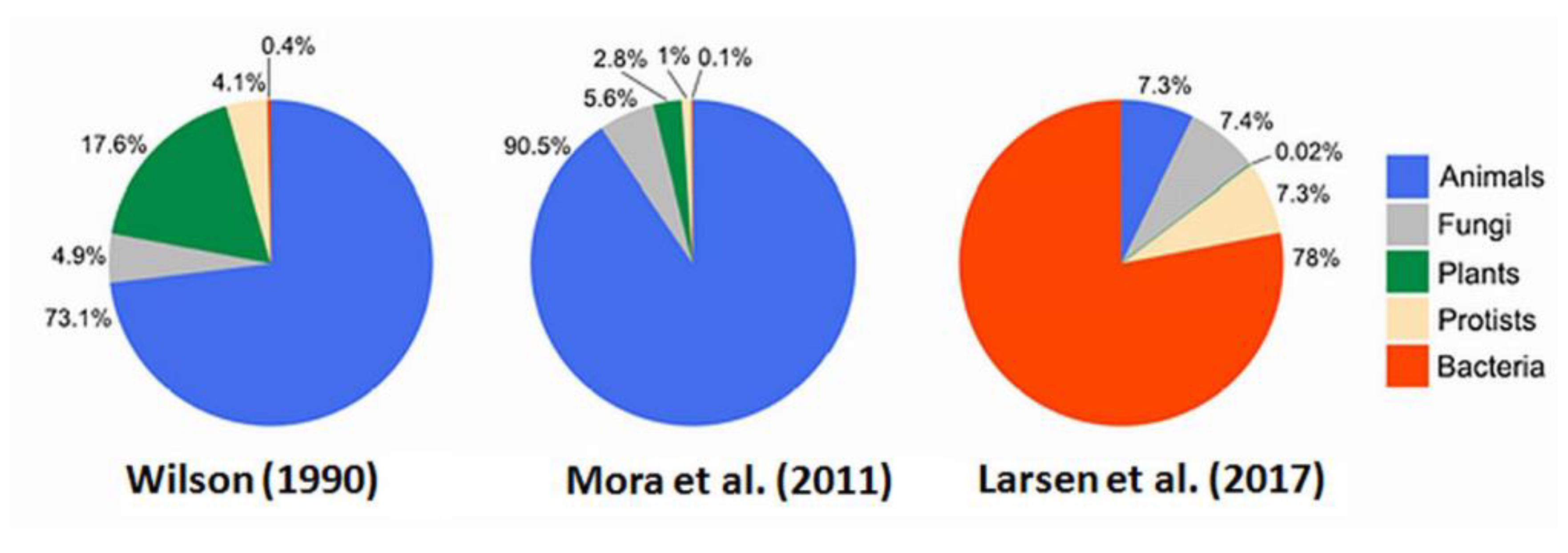
While about two million species have been formally described, global biodiversity recently revised to consider the unique symbionts and parasites of animals produced a new “pie of life” of up to two billion species in toto [92] (cf. Figure 15), a thousand times increase. Some other estimates using scaling laws to predict species go as high as a trillion taxa when all virus and microbes are tallied, e.g., Locey & Lennon (2016) [93]. Any or all of these estimates if based upon the ‘flat-Earth’ land model require up-scaling for terrain, relief, etc., as is proposed herein.

3.6. Topsoil Resource

Returning to the initial questions about the Earth’s organic, microbe-rich topsoil. It is vitally important to determine and to conserve this limited resource or, as Darwin (1881: 39) [31] has it in his swansong book on earthworms: “The vegetable mould [=topsoil humus] which covers, as with a mantle, the surface of the land”. Soils occupy ~81% of land that is not (yet) extreme desert, rock, sand, ice, or waterlogged (19%) (Jackson et al. 1997: tab. 2) [37], and its topsoil fragility is as visualized (Figure 16).

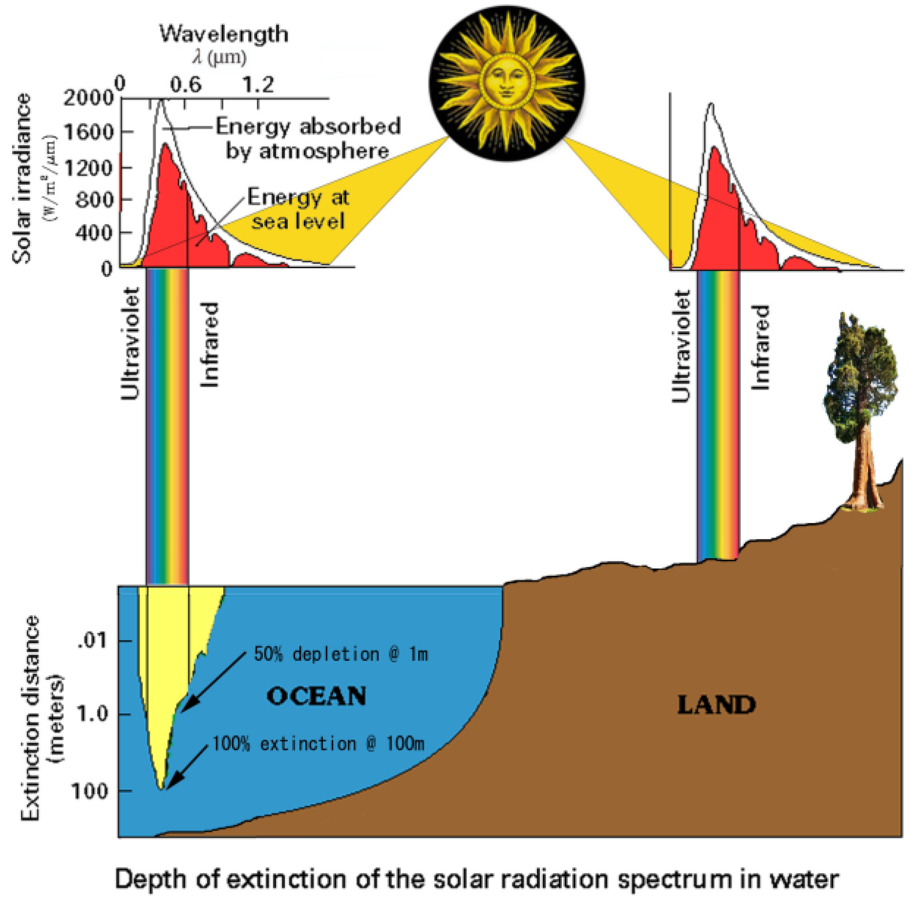
The surface of the Earth is primarily composed of an interface between three essential components, which, in order of volume and levity (antonym of density), are: air, water, and soil that together support abundances of biodiversity in the reverse order. The superficial topsoil that covers all habitable surfaces of the land as a moist, living, breathing skin that manifestly has the highest density and least volume of the three, but overwhelmingly supports the greatest productivity and biomass. The oceans are relatively depauperate, despite moderate volume. The atmosphere has the largest volume with the lowest (negligible) productivity and biomass, much of it transitory: e.g., seeds, insects, spiders, and other aeronauts (volant animals), including cavernicolous bats, microbes, and occasional flying-fish/squid. As well as biota, there is material exchange between these elements in the soil’s moisture and aeration, the silt and (low levels of) dissolved gasses in water, and the humidity and dust in the air. The Sun’s incident visible spectrum energy (for photosynthesis) is depleted by about 25% in the atmosphere, the remainder rapidly reduced by 50% at −1 m and completely extinguished at −100 m depth in salty seawater, whilst on land it is variously absorbed or reflected by plants. Sunlight barely penetrates the superficial soil and litter layers, which is why land plants strive to compete by elevation and extension with the giant Sequoia reaching up to 100 m skywards, while its roots and symbiotic VAM fungi may extend equally deep earthwards (Figure 17).

Clinging to land, autotrophic biofilm, or biocrust contributions to productivity at smaller scales are mostly unquantified. Values [81] of 5 Gt C for ‘cryptogamic covers’, here upped to 10–20 Gt, are higher than the total biomass of mangroves (4 Gt C), seagrasses (0.1 Gt C), and at least double upper estimate of global standing stock of all marine microalgae taxa (0.0075–2.55 Gt C) (cf. Figure 3 of NPP).

3.7. NPP

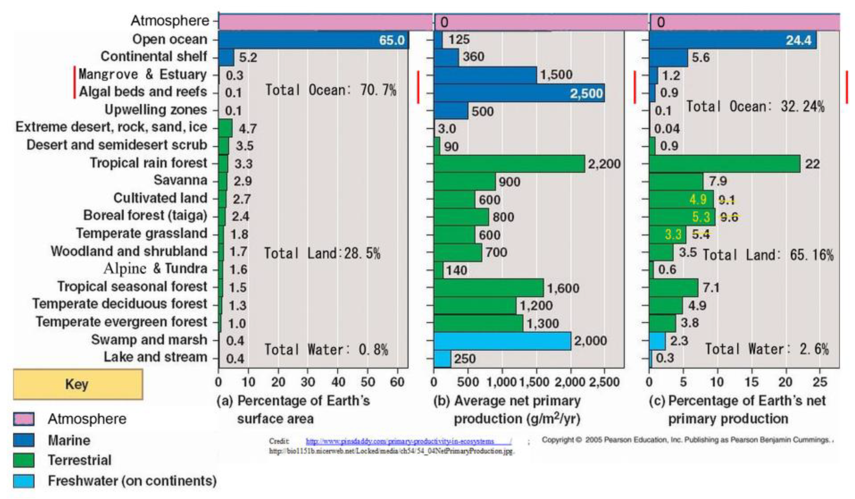
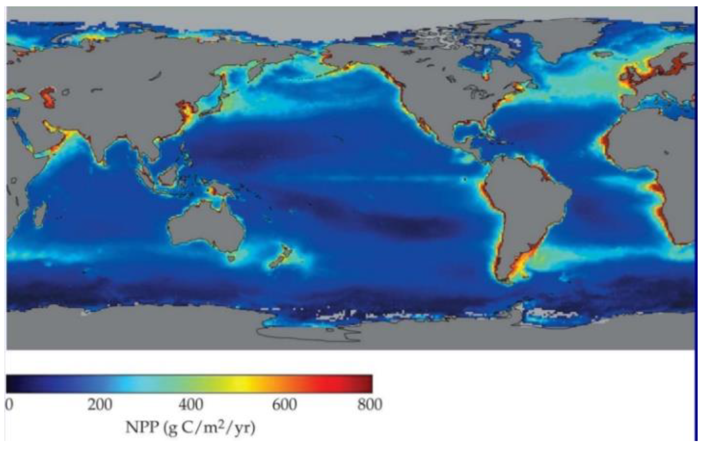
Marine productivity is minor and mainly coastal (e.g., in rockpools), with most open ocean a desolate ‘wet desert’ (Figure 18).

Topsoil naturally relates to net primary productivity (NPP) with land’s contribution, until now put at somewhere around 45–68% (cf. Table 2, Figure 3), yet with correct terrain/topsoil relief factors this would be increased possibly by two or four (or maybe more) to total over 218 Gt C on land. This represents a minimum productivity ratio of soil : sea as 4 : 1 or 80% vs. 20% (

Table 11. Summary of Historical NPP Data Presented with Speculated New Totals.

NPP Totals for 15 Gha Land by Authors	Rate Land C g/m2/yr	Rate Sea C g/m2/yr	Total Land C Gt/yr	Total Sea C Gt/yr	TOTAL NPP Gt C	% Land	% Sea
Duursma & Boisson 1994	144	72	21.6	25.9	48	45	55
Whitman et al. 1989	-	-	48	51	99	48	52
Stiling (1996)	773	152	115	55	170	68	32
UNEP (2002: Table 1.1)	-	-	56.4	48.5	105	54	46
Campbell (2008) recalc.	678.9	138.5	110.3	54.8	165	67	33
NASA (2011)	-	-	93	-	-	-	-
For ~30 Gha land	725.95 *	145.25 *	218	52	270	81%	19%
For ~60 Gha land	725.95 *	145.25 *	436	52	488	89%	11%

* Land and sea rates are based upon the estimated averages of Stiling (1996) [25] and of Campbell (2008) [27] who also included a separate 2% of freshwater productivity, now also diminished by land increase). [Omitted data is Field et al. (1998) [24] as their calculations exclude iced areas].

).

This table shows that NPP per annum has apparently been doubled from 48 Gt to 99 Gt, then up to 170 Gt. Each time with more refinement for the land contribution. The current study continues this trajectory to yield total values of >270 Gt/yr (81% from 30 Gha land), albeit such conclusion requires practical, on-the-ground confirmation. Consideration of finer soil detail and of biocrusts may allow a higher productivity total of 488 Gt C/yr (89% from 60 Gha land).

Pertinent to this are calculations of land productivity per unit area from ecological quadrats that may need to be revised upwards, by ~1–5%, to account for terrain slope/relief (Appendix A). This too applies to earthworm surveys, conventionally tied to a flat 1 m² metric; these too may require a 1–5% increase, but this is minor consideration to their doubling for more refined land surfaces.

Getting to the crux of the Net Primary Productivity (NPP), carbon sequestration, and climate change issue, a recent report stated that: “At a certainty level of 75%, soil C mass will not change if CO₂-induced increase of NPP is limited by nutrients” [71]. The present paper increases soil C mass by increasing soil area/volume, whereas, to the conventional, but problematical, agrichemical advocates this certainty statement would imply that even more synthetic Nitrogen and other chemicals need to be added to soils (cf. Figure 2). To agroecology aficionados, the same statement implies a need to recycle all organic wastes back to the soil to “close the circle”, preferably with more rapid and enhanced nutrient benefits of earthworm vermin-composting, in order to fulfill what Sir Albert Howard (1945) [95] called the ‘Law of Return’.

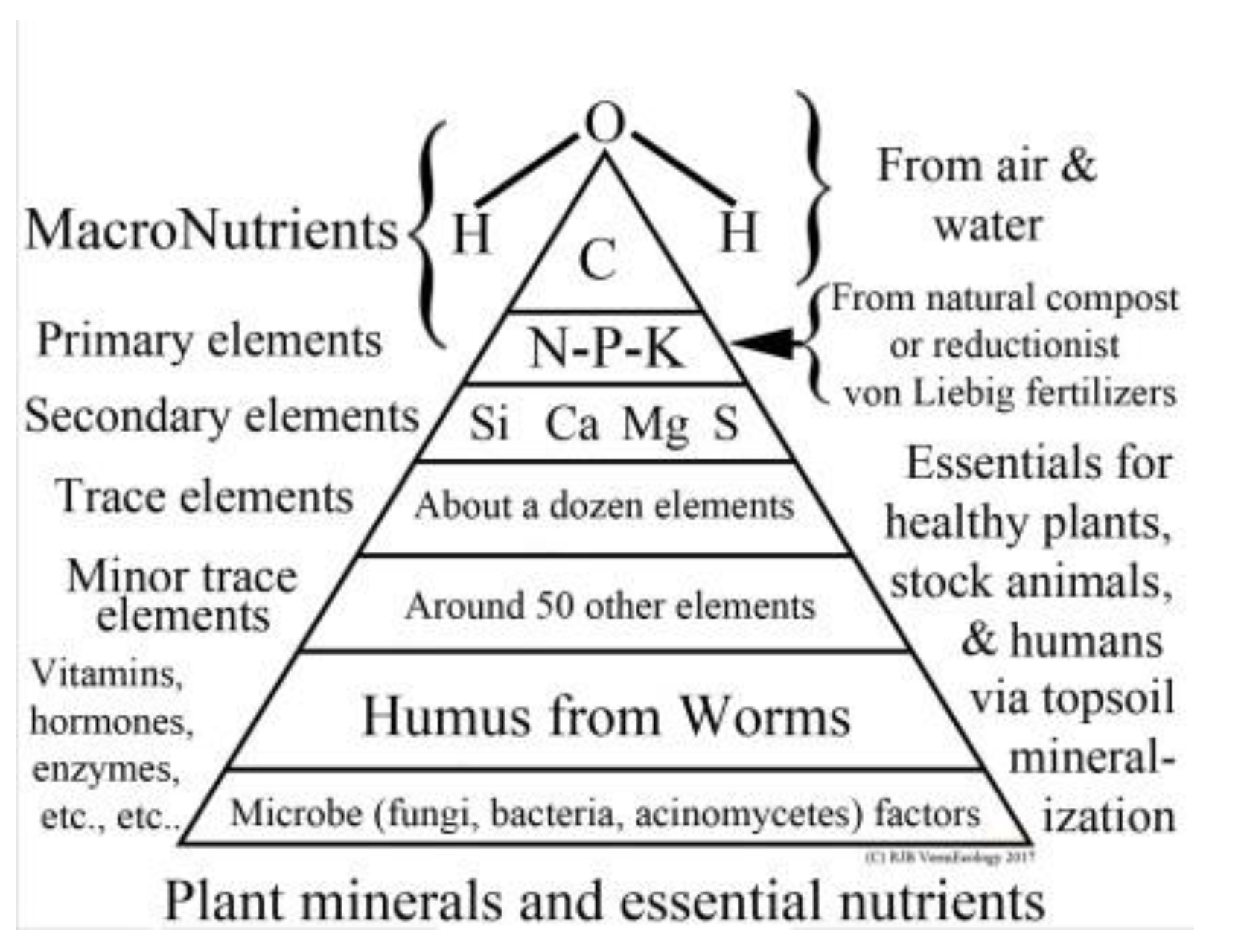
Spontaneous generation has long been debunked, and, similarly, it is not possible for any higher organism to exist without tangible resources as alluded to above: viz. sunlight, water, gasses, nutrients, symbionts, and habitat. Conventionally, soil nutrients are only considered in terms of simplistic von Liebig agrichemicals N-P-K, whereas the proper plant requirements are complex and mainly carbon based, as shown in Permaculture’s nutrient-pyramid charted below (Figure 19).

The context of this recycling is that approximately 50% of global soils are managed, often deleteriously, on chemical farms, in burnt or resown pastures and regrowth forests [84] (cf. Figure 4). The greatest task facing humanity today is to restore topsoils to their full potential with proper management also to repair or reclaim arid and semi-desert lands using Permaculture methods (Mollison, 1988) [96].

3.8. Oceans and Space: Diversions and Distractions to the Problems on Earth

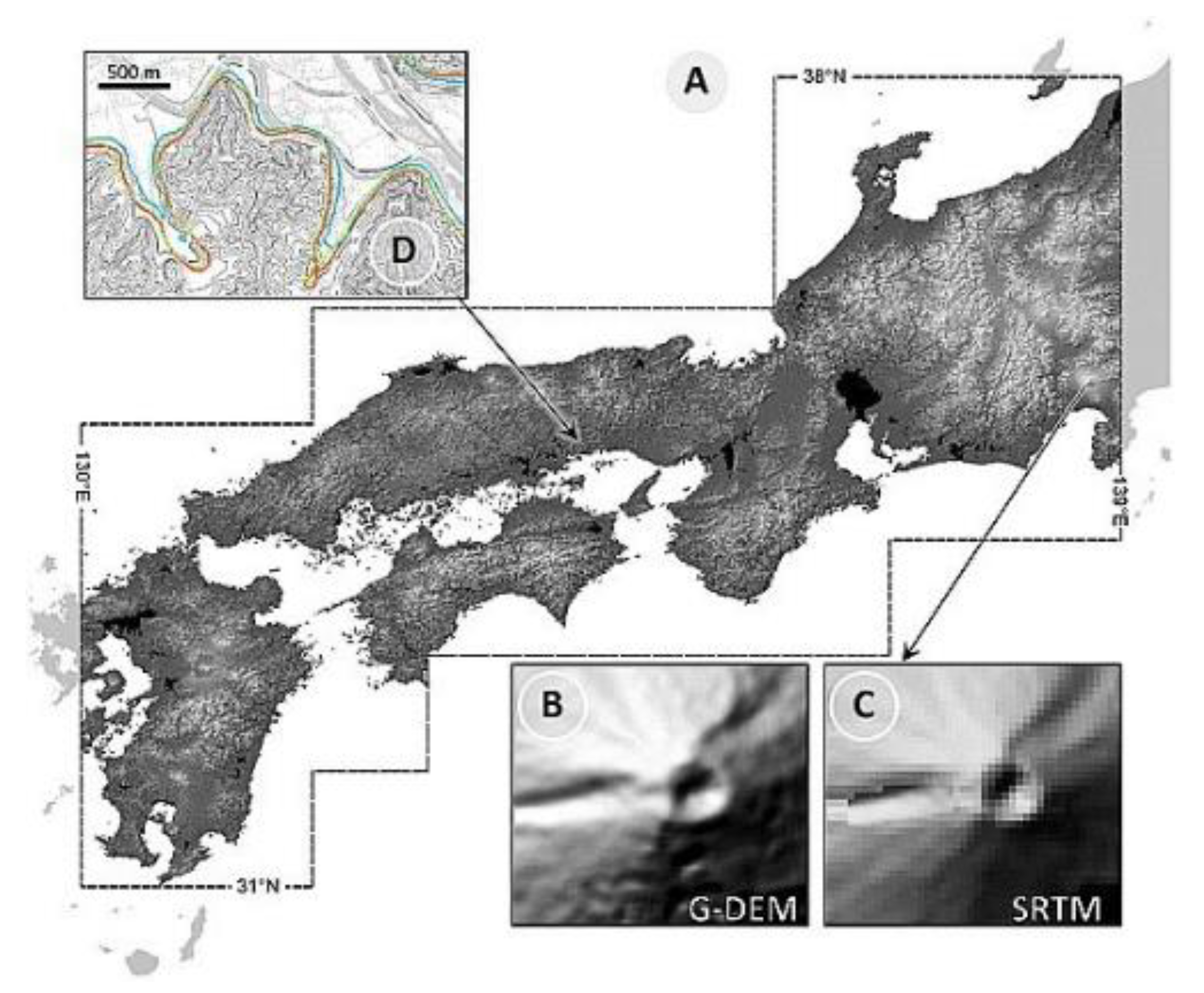
Copley (2017) [97] reveals that the entire ocean floor has now been surveyed to a maximum resolution of around 5 km and that: “NASA’s Magellan spacecraft mapped 98% of the surface of Venus to a resolution of around 100 m. The entire Martian surface has also been mapped at that resolution and just over 60% of the Red Planet has now been mapped at around 20 m resolution. Meanwhile, selenographers have mapped all of the lunar surface at around 100 m resolution and now even at seven metre resolution”. For Earth, global data is available from the 2000 Shuttle Radar Topography Mission (SRTM) and ASTER Global Digital Elevation Model (https://asterweb.jpl.nasa.gov/) with a one arc-second, or about 30-m sampling and some datasets have trees and other non-terrain features removed. However, where is the compiled data for the earth beneath our feet?

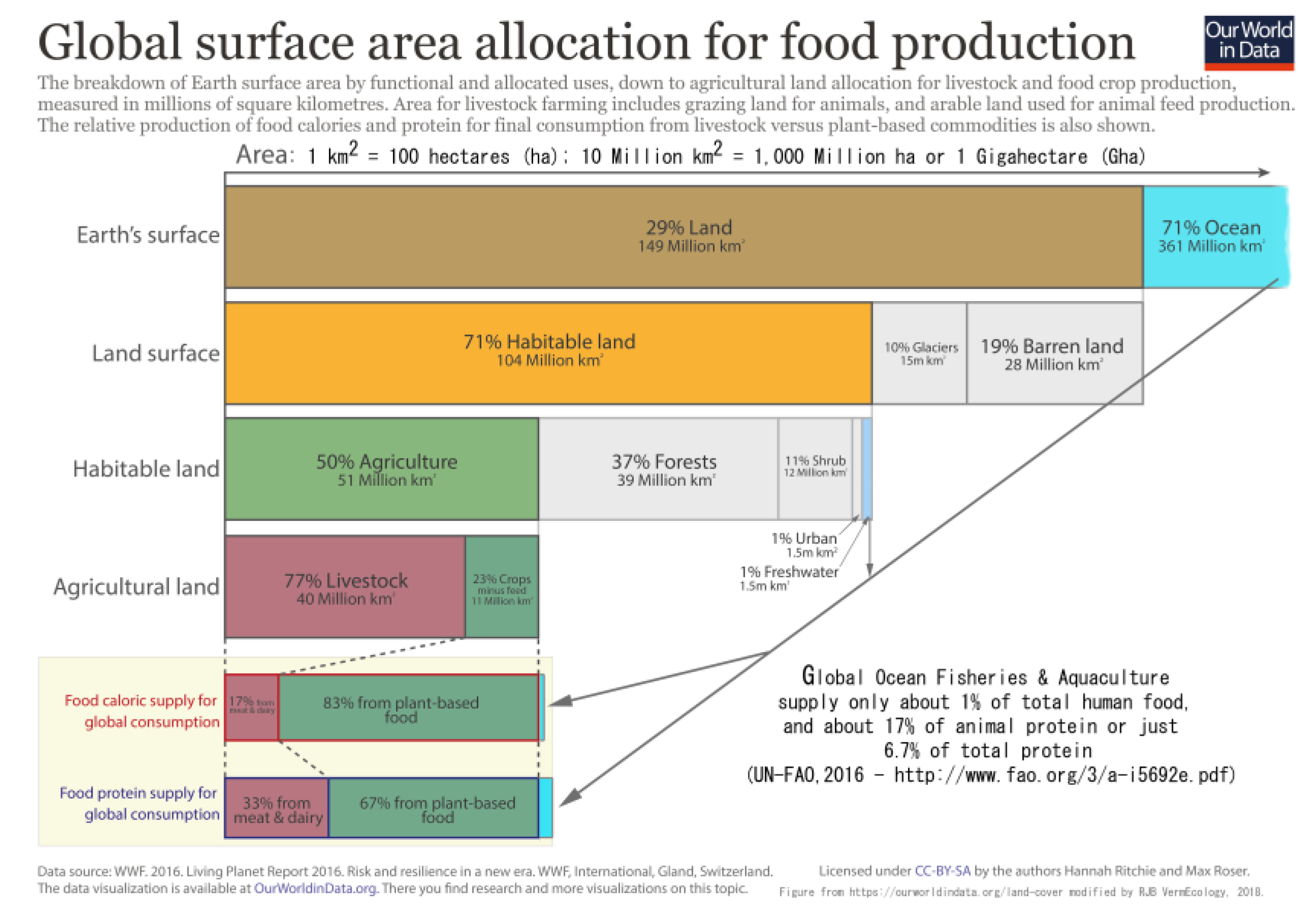
For bathymetry, a surface of 36.066 Gha has a seabed at 2–20-km resolution of 36.138 Gha (Costello et al., 2010: tab. 1) [98]. These authors claim this is important as it somehow relates to ocean fisheries that absolutely supply just <0.5% of human food (the other 0.5% mainly from freshwater aquaculture) [99] (cf. Figure 4). Nevertheless, only the surface of the ocean is oxygenated and exposed to sunlight, thus bathymetry is a completely irrelevant diversion, as are other planets’ topographies, for calculations of primary productivity and biota here on Earth upon which oceanographers and astronomers entirely depend for their survival, as does everyone else. Moreover, marine scientists are unequivocal that the ocean surface does not include the seafloor as they universally quote its surface area as 36 Gha, i.e., the flat interface between the water, the air, and the coastline abutment, even allowing them an (ever increasing) high water mark.

Mars misventures and the latest $10+ billion space telescope (https://jwst.nasa.gov/about.html) aiming yet again to seek “life on planets like Earth” seems much lower priorities as compared to the rapidly declining life on planet Earth of which we yet know but a fraction. The same amount of funding could seed urgently needed Soil Ecology Institutes on each Continent. Similarly, submarine surveys of deep-sea hydrothermal vents costing $ millions to find just a few new species, which will still be there tomorrow, while essential soil species are being lost to erosion daily. Basic equipment for soil survey is a spade. How justifiable is it to dabble in space or deep oceans when we do not yet know how many earthworm species exist on the eponymous Earth, barely nothing of their ecology or conservation status, and even less of their symbiotic/parasitic co-evolutionaries? When the latest report (IPCC 2018) [100] gives us just 12 years to act in order to prevent catastrophic change, studies of deep space or the abyss seem irrational, inessential, and unjustifiable funding choices that misdirect talent and resources from critical issues emanating from and solvable only in and on our homeland turf.

3.9. Worked Example for Samos Island and the Land of the State of Japan

Aristarchus of Samos is credited with the first concept of a spherical Earth revolving around the Sun, an idea later supported by Aristotle on empirical grounds. Appropriately fitting is an attempt to define the topography of Aristarchus’s and Pythagoras’s island of Samos with its central volcanic peak, Vigla, at 1434 m. Its planimetric area of 477.4 km², which, if circular, would give the island a radius of 12.33 km. Thus a crude approximation using Pythagorean hypotenuse as 12.41 km (= new radius) gives a new surface area 483.8 km² that is only about 1.3% larger at the km scale. However, allowing topographic undulations at one metre, or less, to increase area by 50% totals 716.1 km² that may itself be doubled for fractal tortuosity at cm scale to about 1432.2 km² or a 200% increase over original. If hypotenuse/radius is increased 50% to allow for undulating curvatures (i.e., to 18.5), then area is 1075 km², which, if doubled for relief to 2150 km², is substantially (350%) larger.

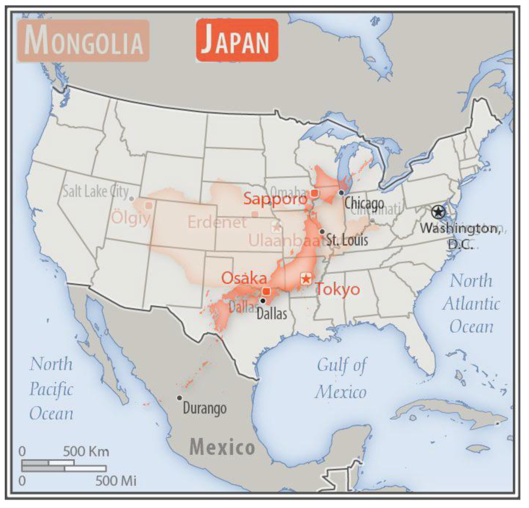
For Japan, [11] its land area is 36,450,000 ha (0.0365 Gha excluding lakes, e.g., Biwako) and average slope of 6.275% (3.59°). If the flat area was considered a circle with base diameter 6812 units, its hypotenuse of 6850 differs by ~0.6% or about 41 units giving a proper diameter of 6853 and a new area of 36,885,132 ha. This extra 435,132 ha (4351 km²), which is the least possible, is only a modest 1.2% extra, but an increase in surface area is likely closer to 400% with finer resolutions, as found in the current study. From the worked examples above, its hilly m² terrain allows 21.25% extra land (at least) and, because soil occupies most of her land, then by 94% cm² tortuosity and then again by mm² 108.2% micro-relief. This gives Japan a practical land of (0.0365 × 1.2125 = 0.044 × 1.94 = 0.085 × 2.082 =) ~0.17 Gha, or × 4.7, which is larger than Mongolia’s flat surface area that is in the realm of 0.15 Gha before its own required readjustments (Figure 20).

3.10. Flaws in Un-Flattening the Earth?

Possible flaws in this land surface argument are that the estimation of quadrupled land area may be excessive, or it may be an underestimation depending upon what scale is chosen. The question is why nobody knows this basic data about Earth? Certainly, the present IPCC or NASA/NOAA values are wrong. Other criticisms may be that Landsat and other satellites, if set to measure perpendicular/planimetric values, make terrain less relevant. Because land productivity calculation is more difficult when compared to ocean or atmosphere budgets, IPCC [101] estimates soil carbon contributions based upon emissions minus atmospheric and oceanic uptake. The residual difference is reasonably ascribed to the land that appears a quite valid method and the ‘missing sink’ discrepancy easily attributed to underestimation of the sub-soil components. Carbon sink calculations when ascribed to biomes may also be artificial due to boundary differences affecting relative % (which may be independent of topography). For example, FAO [102] have grasslands covering 40.5% of land comprised of woody savannah/savannah (13.8%), open/closed shrub (12.7%), non-woodly grassland (8.5%), and tundra (5.7%); whereas, other sources separate these biomes. Calculations relating to carbon stored and released (either eroded or respired) from agriculture, forestry, and other land-use changes, primary productivity and biodiversity studies, however, certainly do need to employ topography details down to cm or mm scale for true tallies.

Regarding soil biomass, as carbon values are drawn from loss-on-ignition (LOI) or Walkley- Black, they may include much of the microbiota (although certainly not the larger megadrile earthworms nor sieved roots/hyphae), whereas microbial measurements often take smaller samples and either extract DNA or use plate cultures to estimate biomass and diversity. Thus, the intermesh of chemical and biotic factors may unintentionally overlap to overstate total carbon in SOM humus.

Conversely, when soil carbon or microbes, or any other organisms, are ascribed to a ‘flat-Earth’ biome then the calculations are invariably and undeniably wide underestimations of both soil depth and of probable land surface area that they occupy both in reality or potentially.

4. Conclusions

“We know more about the movement of celestial bodies than about the soil underfoot”

da Vinci (1500s)

True surface area of uneven land is conclusively raised above conventional 15 Gha to new estimates which vary from 53–75 Gha with a reasoned, arbitrary, Fermi value set at 64 Gha land doubling Earth’s total surface area to 100 Gha. Soil organic carbon (SOC) is then upped to ~9000 Gt, humic SOM to >18,000 Gt, and global biomass, biodiversity, and productivity also elevated. Soil bulk density data are most compelling, since, if the figures differ, then either BD averages are inexact or, as suggested here, the undulating topography is overlooked. As land is one of our three basic biospheric arcs of survival (healthy soil, clean freshwater, breathable air) it is surely important to attempt definition of its fundamental metrics, and, most crucially, the amount of vital organic humus. The classical wisdom and prescient warnings from Plato, Aristotle, da Vinci, Darwin, and Sir Albert Howard may be revisited. The Earth’s inclusive terrain model—with most life and net primary productivity springing from the undulating upper 10 cm of its thin brown line of topsoil—is as summarized in the following schematic (Figure 21).

Geo-morphologists strictly study rough land areas since smooth or flat patches, apart from bodies of water, are extremely rare. Geodesy is concerned with the precise determination of Earth’s land surfaces (called bathymetry in the sea but hereafter considered of lesser importance due to deficits in oxygen, sunlight, nutrients, and consequently, biota). These experts are called upon to confirm these new land surface metrics—as determined with reference to soil bulk densities to quadruple NASA/NOAA’s values—and to calculate the true scope of biomes, thus enabling ecologists to correctly and honestly monitor the Earth’s total living entities, their attributes, and relationships.

References

1. FAO-AGL. Soil Biology Portal. 2004. Available online: https://web.archive.org/web/20040316075918/http://www.fao.org/ag/AGL/agll/soilbiod/consetxt.stm (accessed on 11 November 2018).
2. Blakemore, R.J. Call for a Census of Soil Invertebrates (CoSI). Zool. Middle East 2012, 58, 171–176. Available online: https://vermecology.wordpress.com/2017/04/30/census-of-soil-invertebrated-cosi/ (accessed on 1 May 2017). [CrossRef]
3. Pimentel, D.; Burgess, M. Soil erosion threatens food production. Agriculture 2013, 3, 443–463. [Google Scholar] [CrossRef]
4. Duursma, E.K.; Boisson, M.P.R.M. Global oceanic and atmospheric oxygen stability considered in relation to the carbon-cycle and to different time scales. Oceanol. Acta 1994, 17, 117–141. [Google Scholar]
5. Fierer, N.; Breitbart, M.; Nulton, J.; Salamon, P.; Lozupone, C.; Jones, R.; Robeson, M.; Edwards, R.A.; Felts, B.; Rayhawk, S.; et al. Metagenomic and Small-subunit rRNA Analyses Reveal the Genetic Diversity of Bacteria, Archaea, Fungi, and Viruses in Soil. Appl. Environ. Microbiol. 2007, 73, 7059–7066. [Google Scholar] [CrossRef] [PubMed]
6. Kallmeyer, J.; Pockalny, R.; Adhikari, R.R.; Smith, D.C.; D’Hondt, S. Global distribution of microbial abundance and biomass in subseafloor sediment. Proc. Natl. Acad. Sci. USA 2012, 109, 16213–16216. [Google Scholar] [CrossRef] [PubMed] [Green Version]
7. Blakemore, R.J. VermEcology Japan. 2016. Available online: https://vermecology.wordpress.com/2016/08/11/mountain-day-japans-newest-holiday-falls-flat-according-to-nasa-noaa-usgs-and-japans-own-meti-jaxa-who-all-make-molehills-out-of-mountains/ (accessed on 11 November 2018).
8. Blakemore, R.J. Un-Flattening the Earth, and Worms (or—Aristotle Vindicated at the End of a Flat-Earth). VermEcology Japan. 2017. Available online: https://vermecology.wordpress.com/2017/06/10/un-flattening-the-earth-and-worms/ (accessed on 10 June 2017).
9. Blakemore, R.J. Food for Thought II. 2017. Available online: https://vermecology.wordpress.com/2017/02/22/food-for-thought-ii/ (accessed on 11 August 2017).
10. NOAA. 2018. Available online: https://www.ngdc.noaa.gov/mgg/global/etopo1_ocean_volumes.html (accessed on 11 November 2018).
11. Nunn, N.; Puga, D. Ruggedness: The Blessing of Bad Geography in Africa; The Review of Economics and Statistics; MIT Press: Cambridge, MA, USA, 2009; Available online: https://diegopuga.org/papers/rugged.pdf 2012 (accessed on 11 November 2018).
12. Ripple, W.J.; Wolf, C.; Newsome, T.M.; Galetti, M.; Alamgir, M.; Crist, E.; Mahmoud, M.I.; Laurance, W.F. World Scientists’ Warning to Humanity: A Second Notice. BioScience 2017, 67, 1026–1028. [Google Scholar] [CrossRef] [Green Version]
13. Blakemore, R.J. Environmental Triage. 2018. Available online: vermecology.wordpress.com/2018/07/17/environmental-triage-eco-tri/ (accessed on 27 May 2018).
14. Rockström, J.; Steffen, W.; Noone, K.; Persson, Å.; Chapin, F.S., III; Lambin, E.F. A safe operating space for humanity. Nature 2009, 461, 472–475. [Google Scholar] [CrossRef] [PubMed] [Green Version]
15. Blakemore, R.J. Critical Decline of Earthworms from Organic Origins under Intensive, Humic SOM-Depleting Agriculture. Soil Syst. 2018, 2, 33. [Google Scholar] [CrossRef]
16. De Souza Machado, A.A.; Kloas, W.; Zarfl, C.; Hempel, S.; Rillig, M.C. Microplastics as an emerging threat to terrestrial ecosystems. Glob. Chang. Boil. 2018. [Google Scholar] [CrossRef] [PubMed]
17. Koch, A.; McBratney, A.; Adams, M.; Field, D.; Hill, R.; Crawford, J.; Minasny, B.; Lal, R.; Abbott, L.; O’Donnell, A.; et al. Soil Security: Solving the Global Soil Crisis. Glob. Policy 2013, 4, 434–441. [Google Scholar] [CrossRef] [Green Version]
18. Diamond, M.L.; de Wit, C.A.; Molander, S.; Scheringer, M.; Backhaus, T.; Lohmann, R.; Arvidsson, R.; Bergman, Å.; Hauschild, M.; Holoubek, I.; et al. Exploring the planetary boundary for chemical pollution. Environ. Int. 2015, 78, 8–15. [Google Scholar] [CrossRef] [PubMed] [Green Version]
19. Montgomery, D. Dirt: The Erosion of Civilizations; UC Press: Berkeley, CA, USA, 2008. [Google Scholar]
20. Arsenault, C. Only 60 Years of Farming Left if Soil Degradation Continues. Sci. Am. 2014. Available online: www.scientificamerican.com/article/only-60-years-of-farming-left-if-soil-degradation-continues/ (accessed on 11 November 2018).
21. Jie, D. Chinese Soil Experts Warn of Massive Threat to Food Security. SciDevNet. 5 August 2010. Available online: http://www.scidev.net/global/earth-science/news/chinese-soil-experts-warn-of-massive-threat-to-food-security.html (accessed on 11 July 2018).
22. Withnall, A. Independent Newspaper Article. 2014. Available online: http://www.independent.co.uk/news/uk/home-news/britain-facing-agricultural-crisis-as-scientists-warn-there-are-only-100-harvests-left-in-our-farm-9806353.html (accessed on 10 May 2018).
23. Whitman, W.B.; Coleman, D.C.; Wiebe, W.J. Prokaryotes: The unseen majority. Proc. Natl. Acad. Sci. USA 1998, 95, 6578–6583. [Google Scholar] [CrossRef] [PubMed] [Green Version]
24. Field, C.B.; Behrenfeld, M.J.; Randerson, J.T.; Falkowski, P. Primary production of the Biosphere: Integrating Terrestrial and Oceanic Components. Science 1998, 281, 237–240. [Google Scholar] [CrossRef] [PubMed]
25. Stiling, P. Ecology: Theories and Applications, 2nd ed.; Pearson: London, UK, 1996. [Google Scholar]
26. UNEP. World Atlas of Biodiversity. 2002. Available online: https://archive.org/stream/worldatlasofbiod02groo#page/10/mode/2up (accessed on 11 November 2018).
27. Campbell, N.A.; Reece, J.B. Biology, 7th ed.; Pearson Benjamin Cummings: San Francisco, CA, USA, 2008. [Google Scholar]
28. Falser, D.S.; Westerby, M. Leaf size and angle vary widely across species: What consequences for light interception? New Phytol. 2003, 158, 509–525. [Google Scholar] [CrossRef]
29. Lee, K.E. Earthworms: Their Ecology and Relationships with Soils and Land Use; Academic Press: Sydney, Australia, 1985. [Google Scholar]
30. Richie, H.; Roser, M. Land Cover for Food Production. 2018. Available online: https://ourworldindata.org/land-cover (accessed on 1 September 2018).
31. Darwin, C.R. The Formation of Vegetable Mould through the Action of Worms, with Observation on Their Habits; Murray: London, UK, 1881. [Google Scholar]
32. UN-FAO. 2015. Available online: http://www.fao.org/3/a-i5126e.pdf (accessed on 11 July 2018).
33. Blakemore, R.J. Cosmopolitan Earthworms—An Eco-Taxonomic Guide to the Peregrine Species of the World, 6th ed.; VermEcology: Yokohama, Japan, 2016. [Google Scholar]
34. Blakemore, R.J. Hypolimnus pedderensis redescription. 2008. Available online: www.annelida.net/earthworm/Tasmanian%20Earthworms/Hpedderensis.pdf (accessed on 11 July 2018).
35. Blakemore, R.J. Tokea Orthostichon. IUCN Red List. 2017. Available online: http://dx.doi.org/10.2305/IUCN.UK.2017-2.RLTS.T103192401A103193535.en (accessed on 11 November 2018).
36. Blakemore, R.J. Extinction status of Japan’s first formally described earthworm Amynthas japonicus (Horst, 1883). Bull. Kanagawa Prefect. Mus. (Nat. Sci.) 2018. under review. [Google Scholar]
37. Jackson, R.B.; Moony, H.A.; Schulze, E.D. A global budget for fine root biomass, surface area, and nutrient contents. Proc. Natl. Acad. Sci. USA 1997, 94, 7362–7366. [Google Scholar] [CrossRef] [PubMed] [Green Version]
38. Fortuna, A. The Soil Biota. Nat. Educ. Knowl. 2012, 3, 1. Available online: www.nature.com/scitable/knowledge/library/the-soil-biota-84078125 (accessed on 11 July 2018).
39. Trevors, J.T. One gram of soil: A microbial biochemical gene library. Antonie Van Leeuwenhoek 2010, 97, 99–106. [Google Scholar] [CrossRef] [PubMed]
40. Blakemore, R.J. Wormageddon—Destruction in Our Soils. 2018. Available online: https://vermecology.wordpress.com/2018/05/27/wormageddon-destruction-in-our-soils/ (accessed on 11 November 2018).
41. NASA. 2011. Available online: https://earthobservatory.nasa.gov/Features/CarbonCycle/ (accessed on 1 November 2018).
42. Blakemore, R.J. Eco-Taxonomic Profile of an Iconic Vermicomposter—The ‘African Nightcrawler’ Earthworm, Eudrilus eugeniae (Kinberg, 1867). Afr. Invertebr. 2015. [Google Scholar] [CrossRef]
43. ABC (Australian Broadcasting Corporation). 2014. Available online: www.abc.net.au/news/rural/2014-03-23/johan-boucan-soils-feed-the-world/5332570 (accessed on 11 July 2018).
44. Kamphorst, E.C.; Jetten, V.; Guerif, J.; Pitkanen, J.; Iversen, B.V.; Douglas, J.T.; Paz, A. Predicting depressional storage from soil surface roughness. Soil Sci. Soc. Am. J. 2000, 64, 1749–1758. [Google Scholar] [CrossRef]
45. Tarolli, P.; Sofia, G.; Ellis, E. Mapping the topographic fingerprints of humanity across Earth. Eos 2017, 98. [Google Scholar] [CrossRef]
46. Swatantran, A.; Tang, H.; Barrett, T.; DeCola, P.; Dubyah, R. Rapid, High-Resolution Forest Structure and Terrain Mapping over Large Areas using Single Photon Lidar. Sci. Rep. 2016, 6, 28277. [Google Scholar] [CrossRef] [PubMed] [Green Version]
47. Jenness, J.S. Calculating landscape surface area from digital elevation models. Wildl. Soc. Bull. 2004, 32, 829–839. [Google Scholar] [CrossRef]
48. Hodgson, M.E. What cell size does the computed slope/aspect angle represent? Photogramm. Eng. Remote Sens. 1995, 6, 513–517. [Google Scholar]
49. Kretzschmar, A. Description des galeries de vers de terre et variations saisonnières des réseaux (observations en conditions naturelles). Rev. Ecol. Biol. Sol. 1982, 19, 579–591. [Google Scholar]
50. Overbeek, J.T.G. Surface Area Determinations; Butterworths: London, UK, 1970. [Google Scholar]
51. Ying, L.-X.; Shen, Z.-H.; Piao, S.-L.; Liu, Y.; Malanson, P. Terrestrial surface-area increment: The effects of topography, DEM resolution, and algorithm. Phys. Geogr. 2014, 35, 297–312. [Google Scholar] [CrossRef]
52. Moore, J.G.; Mark, R.K. World slope map. EOS 1983, 67, 1353–1362. [Google Scholar] [CrossRef]
53. Milevski, I.; Milevska, A. Improvement of slope angle models derived from medium to fine-scale DEM’s. Key study: Skopje area. In Geomorphometry for Geosciences; Jasiewicz, J., Zwolinski, Z., Mitasova, H., Hengel, T., Eds.; Geomorphometry.org: Poznan, Poland, 2015; pp. 91–94. [Google Scholar]
54. Anon. Developing Surface Area Final Report. Planning Department of Himachal Pradesh, India. 2018. Available online: http://hpplanning.nic.in/Developing%20Surface%20Area_FinalReport_CGRT.pdf (accessed on 11 July 2018).
55. Rashid, H. 3-D Surface-Area Computation of the State of Jammu & Kashmir Using Shuttle Radar Topographic Mission (SRTM) Data in Geographical Information System (GIS). J. Geomat. 2010, 4, 77–82. [Google Scholar]
56. Nogués-Bravo, D.; Araújo, M.B. Species richness, area and climate correlates. Glob. Ecol. Biogeogr. 2006, 15, 452–460. [Google Scholar] [CrossRef]
57. Zhang, Y.; Zhao, Y.C.; Shi, X.Z.; Lu, X.X.; Yu, D.S.; Wang, H.J.; Sun, W.X.; Darilek, J.L. Variation of soil organic carbon estimates in mountain regions: A case study from Southwest China. Geoderma 2008, 146, 449–456. [Google Scholar] [CrossRef]
58. Sutton, P.; Lopez, M. Ironing out Colorado. GeoWorld, 2003; p. 58. Available online: http://www.innovativegis.com/basis/supplements/bm_dec_02/ironing_colorado.htm (accessed on 11 July 2018).
59. Martin, Y.; Valeo, C.; Tait, M. Centimetre-scale digital representations of terrain and impacts on depression storage and runoff. Catena 2008, 75, 223–233. [Google Scholar] [CrossRef]
60. Bramorski, J.; De Maria, I.C.; Crestana, S. Relations between soil surface roughness, tortuosity, tillage treatments, rainfall intensity and soil and water losses from a red yellow latosol. Revista Brasileira De Ciência Do Solo 2012, 36, 1291–1297. [Google Scholar] [CrossRef]
61. Boiffin, J. La Degradation Structural des Couches Superficielles du sol Sous L’action des Pluies. Ph.D. Thesis, de L’institut National Agronomique Paris-Grignon, Paris, France, 1984. Available online: http://prodinra.inra.fr/ft?id=66CEBB9C-F463-4874-A4B6-36AE07517A65 (accessed on 11 July 2018).
62. Thomsen, L.M.; Baartman, J.E.M.; Barneveld, R.J.; Starkloff, T.; Stolte, J. Soil surface roughness: Comparing old and new measuring methods and application in a soil erosion model. Soil 2015, 1, 399–410. [Google Scholar] [CrossRef]
63. Helming, K.; Jeschke, W.; Storl, J. Surface Reconstruction and Change Detection for Agricultural Purposes by Close Range Photogammetry and Remote Sensing. In Proceedings of the International Society for Photogrammetry, XXIX Congress, Washington, DC, USA, 1992; Available online: http://www.isprs.org/proceedings/XXIX/congress/part5/610_XXIX-part5.pdf (accessed on 11 July 2018).
64. Mirzaei, M.R.; Ruy, S.; Ziarati, T.; Salehi, A. Monitoring of soil roughness caused by rainfall using stereo-photogrammetry. Int. Res. J. Appl. Basic Sci. 2008, 3, 322–388. [Google Scholar]
65. Grims, M.; Atzberger, T.B.; Strouss, P.; Mansberger, R. Low-cost Terrestrial Photogrammetry as a Tool for a Sample-Based Assessment of Soil Roughness. PGF, Stuttgart. 2014. Available online: http://www.dgpf.de/pfg/2014/pfg2014_5_grims.pdf (accessed on 11 July 2018).
66. Koiter, A.J. Short-Term Carbon Dioxide and Nitrous Oxide Flux Following Tillage of the Clay Soil in the Red River Valley in Southern Manitoba. Masters’ Thesis, Department of soil Science, University of Manitoba, Winnipeg, MB, Canada, 2008. Available online: https://mspace.lib.umanitoba.ca/xmlui/bitstream/handle/1993/8046/Koiter_Short-term_carbon.pdf?sequence=1&isAllowed=y (accessed on 11 July 2018).
67. De Jonge, H.; Mittelmeijer-Hazeleger, M.C. Adsorption of CO2 and N2 on Soil Organic Matter: Nature of Porosity, Surface Area, and Diffusion Mechanisms. Environ. Sci. Technol. 1996, 30, 408–413. [Google Scholar] [CrossRef]
68. Chiou, C.T.; Lee, J.-F.; Boyd, S.A. The surface area of soil organic matter. Environ. Sci. Technol. 1990, 24. [Google Scholar] [CrossRef]
69. Hoechstetter, S.; Walz, U.; Dang, L.H.; Thinh, N.X. Effects of topography and surface roughness in analyses of landscape structure—A proposal to modify the existing set of landscape metrics. Landsc. Online 2008, 3, 1–14. [Google Scholar] [CrossRef]
70. Asner, G.P.; Scurlock, J.M.O.; Hicke, J.A. Global synthesis of leaf area index observations: Implications for ecological and remote sensing studies. Glob. Ecol. Biogeogr. 2003, 12, 191–205. [Google Scholar] [CrossRef]
71. Köchy, M.; Heiderer, R.; Freibauer, A. Global distribution of soil organic carbon—Part 1: Masses and frequency distributions of SOC stocks for the tropics, permafrost regions, wetlands, and the world. Soil 2015, 1, 351–365. [Google Scholar] [CrossRef]
72. Pribyl, D.W. A critical review of the conventional SOC to SOM conversion factor. Geoderma 2010, 156, 75–83. [Google Scholar] [CrossRef]
73. Lal, R. Sequestration of atmospheric CO2 in global carbon pools. Energy Environ. Sci. 2008, 1, 86–100. [Google Scholar] [CrossRef]
74. Blakemore, R.J. Veni, Vidi, Vermi… I. On the Contribution of Darwin’s ‘Humble Earthworm’ to Soil Health, Pollution-Free Primary Production, Organic ‘Waste’ Management & Atmospheric Carbon Capture for a Safe and Sustainable Global Climate. VermEcology Occasional Papers. 2016, Volume 2, pp. 1–34. Available online: http://orgprints.org/31188/3/VVV%20part-I.pdf (accessed on 10 May 2018).
75. Carvalhais, N.; Forkel, M.; Khomik, M.; Bellarby, J.; Jung, M.; Migliavacca, M.; Mu, M.; Saatchi, S.; Santoro, M.; Thurner, M.; et al. Global covariation of carbon turnover times with climate in terrestrial ecosystems. Nature 2014, 514, 213–217. [Google Scholar] [CrossRef] [PubMed]
76. IPCC. Fourth Assessment Report: Climate Change (AR4). 2007. Available online: http://www.ipcc.ch/report/ar4/ (accessed on 11 July 2018).
77. Mokany, K.; Raison, R.J.; Prokushkin, A. Critical analysis of root: Shoot ratios in terrestrial biomes. Glob. Chang. Biol. 2005, 12, 84–96. [Google Scholar] [CrossRef]
78. Bolinder, M.A.; Angers, D.A.; Dubuc, J.P. Estimating shoot to root ratios and annual carbon in soils for cereal crops. Agric. Ecosyst. Environ. 1997, 63, 61–66. [Google Scholar] [CrossRef]
79. Robinson, D. Scaling the depths: Below-ground allocation in plants, forests and biomes. Funct. Ecol. 2004, 18, 290–295. [Google Scholar] [CrossRef]
80. Batjes, N.H. Total carbon and nitrogen in the soils of the world. J. Soil Sci. 1996, 47, 151–163. [Google Scholar] [CrossRef]
81. Bar-On, Y.M.; Phillips, R.; Milo, R. The biomass distribution on Earth. Proc. Natl. Acad. Sci. USA 2018. [Google Scholar] [CrossRef] [PubMed]
82. Blakemore, R.J. Nature Article to Commemorate Darwin’s Birthday. 2017. Available online: https://vermecology.wordpress.com/2017/02/12/nature-article-to-commemorate-charles-darwins-birthday-on-12th-feb/ (accessed on 22 February 2017).
83. Sundquist, E.T.; Visser, K. The Geologic History of the Carbon Cycle. Treatise on Geochemistry; Schlesinger, W.H., Holland, H.D., Turekian, K.K., Eds.; Elsevier: Amsterdam, The Netherlands, 2003; Volume 8, pp. 425–472. ISBN 0-08-043751-6. Available online: https://people.ucsc.edu/~mdmccar/migrated/ocea213/readings/02_C_cycle_Long_T/Sundquist_&_Visser_Geologic_History_of_C_Cycle_TOG_Vol8_chpt9_OCR_Converted.pdf (accessed on 11 July 2018).
84. Scharlemann, J.P.W.; Tanner, E.V.J.; Heiderer, R.; Kapos, V. Global soil carbon: Understanding and managing the largest terrestrial carbon pool. Carbon Manag. 2014, 5, 81–89. [Google Scholar] [CrossRef]
85. Wilson, R.W.; Millero, F.J.; Taylor, J.R.; Walsh, P.J.; Christensen, V.; Jennings, S.; Grosell, M. Contribution of fish to the marine inorganic carbon cycle. Science 2009, 323, 359–362. [Google Scholar] [CrossRef] [PubMed]
86. Ross, K.F.A.; Billing, E. The Water and Solid Content of Living Bacterial Spores and Vegetative Cells as Indicated by Refractive Index Measurements. Microbiology 1956, 16, 418–425. [Google Scholar] [CrossRef] [PubMed]
87. Kirschner Laboratory Paper. 2018. Available online: http://kirschner.med.harvard.edu/files/bionumbers/Calculated%20values%20for%20percent%20dry%20weight%20of%20bacterial%20cells.pdf (accessed on 11 September 2018).
88. Smil, V. Harvesting the Biosphere; MIT Press: Cambridge, MA, USA, 2011; Available online: https://www.gatesnotes.com/Books/Harvesting-The-Biosphere (accessed on 11 July 2018).
89. AGCI (Aspen Global Change Institute USA). Available online: www.agci.org/earth-systems/biosphere (accessed on 1 September 2018).
90. Woese, C.R.; Kandler, O.; Wheelis, M.L. Towards a natural system of organisms: Proposal for the domains Archaea, Bacteria, and Eucarya. Proc. Natl. Acad. Sci. USA 1990, 87, 4576–4579. [Google Scholar] [CrossRef] [PubMed]
91. Mora, C.; Tittensor, D.P.; Adl, S.; Simpson, A.G.B.; Worm, B. How Many Species Are There on Earth and in the Ocean? PLoS Biol. 2011, 9, e1001127. [Google Scholar] [CrossRef] [PubMed]
92. Larsen, B.B.; Miller, E.C.; Rhodes, M.R.; Wiens, J.J. Inordinate Fondness Multiplied and Redistributed: The Number of Species on Earth and the New Pie of Life. Q. Rev. Biol. 2017, 92, 229–265. [Google Scholar] [CrossRef]
93. Locey, K.J.; Lennon, J.T. Scaling laws predict global microbial diversity. Proc. Natl. Acad. Sci. USA 2016, 113, 5970–5975. [Google Scholar] [CrossRef] [PubMed]
94. Blakemore, R.J. Food for Thought. 2015. Available online: https://vermecology.wordpress.com/2015/12/09/food-for-thought-earthworms-support-the-globe-on-their-very-narrow-shoulders/ (accessed on 5 December 2015).
95. Howard, A. An Agricultural Testament; Oxford University Press: London, UK, 1947. [Google Scholar]
96. Mollison, B. Permaculture: A Designers’ Manual; Tagari Publications: Sisters Creek, Australia, 1988. [Google Scholar]
97. Copley, J. Just how little do we know about the ocean floor? Conversation 2014. Available online: https://theconversation.com/just-how-little-do-we-know-about-the-ocean-floor-32751 (accessed on 11 July 2018).
98. Costello, J.; Cheung, A.; De Hauwere, N. Surface Area and the Seabed Area, Volume, Depth, Slope, and Topographic Variation for the World’s Seas, Oceans, and Countries. Environ. Sci. Technol. 2010, 44, 8821–8828. [Google Scholar] [CrossRef] [PubMed]
99. UN-FAO. 2016. Available online: http://www.fao.org/3/a-i5692e.pdf (accessed on 11 July 2018).
100. IPCC. Special Report. 2018. Available online: http://report.ipcc.ch/sr15/pdf/sr15_spm_final.pdf (accessed on 11 July 2018).
101. IPCC. Fifth Assessment Report: Climate Change. 2014. Available online: http://www.ipcc.ch/report/ar5/ (accessed on 11 July 2018).
102. FAO. 2005. Available online: http://www.fao.org/docrep/008/y8344e/y8344e05.htm (accessed on 11 July 2018).
103. Hayakawa, Y.S.; Oguchi, T.; Lin, Z. Comparison of new and existing global digital elevation models: ASTER G-DEM and SRTM-3. Geophys. Res. 2008, 35, L17404. [Google Scholar] [CrossRef]
104. Mandelbrot, B. The Fractal Geometry of Nature; W.H. Freeman and Co.: New York, NY, USA, 1983; pp. 25–33. ISBN 978-0-7167-1186-5. Available online: https://users.math.yale.edu/~bbm3/web_pdfs/howLongIsTheCoastOfBritain.pdf (accessed on 11 July 2018).
Figure 1. (a) Hiroshige Utagawa’s 1833 ukiyo-e print: “Bandits’ Paradise: Hakone on the Tokaido” (looking towards Mt Fuji), it intuitively and stylistically demonstrates undulations with a patchwork mosaic of landforms and also shows how people closely follow each other, rarely looking out beyond the pack for tribal reasons of safety; (b) NASA/NOAA’s alternate ‘flat-Earth’ view of this landscape; remarkably, most current totals of biodiversity, productivity, plus carbon and other nutrient budgets based upon their flat linear-model are consequently incorrect, widely underestimating true values.
Soilsystems 02 00064 g001
Figure 2. Graphic of eco-triage [13,14,18]; although all are ecologically interlinked, global climate change (1) is not the most important nor most urgent of environmental problems (cf. ?6, 8–9).
Soilsystems 02 00064 g002
Figure 3. Net primary productivity (NPP) contributions of ‘flat-Earth’ biomes (corrected in yellow); despite contrary claims, mangroves or coral reef (in red) are of minimal importance, just ~2% overall; ditto water. [After [27] (fig. 54.4) from [25] “Stiling (1996), Ecology: Theories and Applications”].
Soilsystems 02 00064 g003
Figure 4. Conventional land allocations (just ~1% urban); while relative land proportions may not vary greatly [30], certainly land as a whole requires increasing for terrain and soil relief. Agricultural crops also supply nutrients for aquaculture that increases yearly but it is still a minor food source [9].
Soilsystems 02 00064 g004
Figure 5. Soil biodiversity, enhanced at meso and, micro, or nano scales (credits in [40] https://vermecology.wordpress.com); each cm3 of soil comprises 1000 × 1 mm3 and so ad infinitum thus superficial structures of terrain and intimate or intricate details to soil depth matter greatly.
Soilsystems 02 00064 g005
Figure 6. Red line Digital Elevation Models (DEMs) include either or both Digital Surface Model (DSM) and Digital Terrain Model (DTM), as shown in this figure (modified with permission after http://www.charim.net/datamanagement/32: fig. 1); also shown is simplistic and unrepresentative NASA/NOAA ‘flat-Earth’ model upon which most current (incorrect) global soil, biodiversity, and primary productivity estimates are formulated (cf. Figure 1).
Soilsystems 02 00064 g006
Figure 7. Real-time photon scale LiDAR scan modified from [46] (fig. 4 CC-BY).
Soilsystems 02 00064 g007
Figure 8. Classical and, perforce, simplistic DEM from Jenness (2004: figs. 4a, b) [47] as compared to impossible complexity of earthworm casts from Darwin (1881: figs. 3, 4) [31]; straight lines are rare in Nature and models need to allow for arc length, regardless if concave or convex. In reality, possibly only laser scanning can accurately record extent and surface areas of natural events and forms. (Note too that worms’ surface castings indicate tunneling and channeling of aerating sub-surface voids).
Soilsystems 02 00064 g008
Figure 9. Slope or model concepts: (a) a circle and square of same area; (b) foreshortening on blue base line of a sloped red or black hypotenuse (=diameter of circle or side of a square); (c) basic Ti model of sloped area over actual base area; (d) projection errors for quadrat surveys; (eh) sinuous or tortuous topography/relief at various scales showing how straight (red) line models invariably miss curve complexity as found in Nature. Respective corrections to quadrats, the stalwarts for ecological surveys, and for DEM arcs are advocated, flagged, and/or newly applied herein (see Appendix A).
Soilsystems 02 00064 g009
Figure 10. Reactive carbon cycle relating to global warming and climate change with bedrock added; after NASA 2011 [41] from US DoE image as per [74] (fig. 4); herein, terrestrial components are questioned as widely underestimated due to ignored surface undulation and sub-soil factors allowing productivity much higher on land than in sea. Variable gas fluxes are complex and largely irrelevant: only net soil carbon storage matters and this is mainly on land and in the neglected soil.
Soilsystems 02 00064 g010
Figure 11. After Scharlemann et al. (2014: tab. 1, fig. 3 CC-BY— tandfonline.com/terms-and-conditions) [84] of terrestrial organic carbon in twelve IPCC-defined climatic regions in above- (phytomass) and below-ground (soil carbon to 1 m depth). Both these totals increase substantially when terrain and relief are taken into consideration as already shown herein. Flammable above-ground forest trees or savannah grasses are not the major nor most long-term C stores, as is often assumed, unlike intractable SOC/humic-SOM that may be resilient for 1000 s of years.
Soilsystems 02 00064 g011
Figure 12. Latest global biomass C estimate from Bar-On et al. (2018: tab. S1, fig. S4) [81] modified in red (as acknowledged by author Dr Ron Milo pers. emails 16 July 2018), that totaled ~545.2 Gt C with 97.2% terrestrial vs. 2.8% oceanic which compares to data by Duursma & Boission (1994) [4] of about 99.78% land vs. 0.22% sea for Earth’s total living organisms. In contrast, Dr Sylvia Earle (2009 https://oceantoday.noaa.gov/sylviaearle/) still claims ocean as “home for about 97% of life in the world, maybe in the universe”. The present study quadruples the biomass total to above 2000 Gt C on land.
Soilsystems 02 00064 g012
Figure 13. A phylogenetic tree of living things, based on RNA data and proposed by Carl Woese, showing the separation of Bacteria, Archaea, and Eukaryota (source: https://en.wikipedia.org/wiki/File:Phylogenetic_tree.svg based on Woese et al. 1990 [90] CC-BY).
Soilsystems 02 00064 g013
Figure 14. Snapshot of biodiversity totals from Mora et al. (2011) [91] (ex Wikipedia from en.wikipedia.org/wiki/File:Mora_2011_Predicted_and_Unpredicted_species.png); this shows that land already had much higher catalogue than oceans: 1.2 v 0.19 million taxa despite the oceans being much better systematically surveyed than soils following the 10 yrs, $1 billion CoML 2010 (http://coml.org) (cf. [2]). Land biota totals may easily be doubled for terrain and rugged soil relief.
Soilsystems 02 00064 g014
Figure 15. Progressive estimates of the proportions of biotic taxa showing our fundamental lack of knowledge of Life on Earth, especially of the bacteria and fungi that are dominant in most soils (modified from Larsen et al. 2017 [92]). Note too that higher plants often have ‘microspecies’.
Soilsystems 02 00064 g015
Figure 16. The moon, air, H2O, and soil [94]; topsoil previously estimated as ~4000 Gt of SOM humus is herein raised about four-fold to >17,810 Gt SOM, nearly equivalent to annual global rainfall; even so, it still requires much more attention and conservation efforts as it is yet the most limited and most polluted of all three vital resources (viz. healthy topsoil, freshwater and clean air).
Soilsystems 02 00064 g016
Figure 17. Photosynthesis potential of flat ocean as compared to undulating and verdant land (imagearchive.usgs.gov/archive/sites/ks.water.usgs.gov/images/studies/surface_water/solar_irradiance/ijc.fig1.gif modified with CC-BY permissions). Even if light is adequate, O2, nutrients, and minerals are highly restricted in the open oceans thus limiting marine biomass and productivity mainly to coastal fringes (http://science.sciencemag.org/content/281/5374/237/F1 and see Supplementary file). Life on Earth likely originated in geothermal hot springs on land, yet as in Darwin’s “warm little pond” (http://adsabs.harvard.edu/abs/2016AGUFM.P32A..02D and see [2]).
Soilsystems 02 00064 g017
Figure 18. Most marine NPP is due to soil run-off (as presented by NASA’s SeaWiFS Project 2003, www.nasa.gov/vision/earth/environment/ocean_plants_21.html, accessed 11 November 2018).
Soilsystems 02 00064 g018
Figure 19. Plant nutrient pyramid (from https://vermecology.wordpress.com 2018 [40]); Carbon in plants and soil is by far the most important element; atmospheric N2 is used by nitrogen-fixing soil microbes and it is also released by weathering of soils, the rates of which are both substantially underestimated without terrain or topsoil relief being factored in.
Soilsystems 02 00064 g019
Figure 20. Recalibrated Japan’s area exceeds current Mongolia’s: relative sizes overlain on flat USA.
Soilsystems 02 00064 g020
Figure 21. New view of Earth’s meaningful surface area (modified from www.ngdc.noaa.gov/mgg/global/etopo1_surface_histogram.html, accessed 11 November 2018).
Soilsystems 02 00064 g021