Correlations of Seismic Velocities and Elastic Moduli with Temperature in Superhot and Enhanced Geothermal Systems

Abstract

This paper presents correlations derived by linear regression analysis of seismic velocities V_P and V_S and elastic moduli E_P and E_S with temperature in Los Humeros superhot (SHGS) and Acoculco enhanced (EGS) geothermal systems at depths down to 3 km below the surface and temperatures up to approximately 400 °C. In Los Humeros, the seismic velocity models were derived from the inversion of legacy active seismic survey data acquired in 1998, as well as from passive seismic monitoring and ambient seismic noise interferometry carried out during 2017–2019 by the GEMex consortium. In the Acoculco EGS, ambient seismic noise data were used. Steady-state formation temperatures were re-evaluated during and after the end of the GEMex project using measurements provided as a courtesy of the Federal Electricity Commission of Mexico (CFE). The density data needed for the calculation of elastic moduli were provided by the GEMex consortium, as derived from the inversion of regional and local gravity surveys. The analysis indicated that statistically significant correlations of seismic parameters to temperature exist in the vertical direction, namely exponential in Los Humeros superhot and logarithmic in Acoculco EGS, but no correlation was evident in the horizontal direction. This result suggests an indirect relationship among the considered variables due to interdependence on other parameters, such as pressure and vapor saturation. As the analysis was performed using only data obtained from sensing-at-surface methods, without direct geophysical calibration at depth, a distributed fiber-optic seismic and temperature sensing system at both surface and downhole is proposed for active-source and passive seismic monitoring, and seismic-while-drilling by the drill-bit source is considered for reverse vertical seismic profile (RVSP) recording whenever possible for future high-temperature geothermal applications.

1. Introduction

This work has been carried out in the framework of the EU2020 GEMex project in an effort to seek possible correlations between rock elastic properties and formation temperature in the geothermal fields of Los Humeros (superhot) and Acoculco (EGS) in Mexico. The temperature dependence of seismic velocities has been previously studied in the geothermal fields of Krafla (Iceland), Hengill (Iceland), and Dixie Valley (Nevada, NV, USA), as described below.

Jones et al. [1] exhibited the dependence of seismic velocities on reservoir parameters, such as pressure, saturation, and temperature, in granite and sandstone. They indicated that strong dependence of seismic velocities on temperature can occur due to associated changes in saturation and thermal stress fracturing.

Kristinsdóttir et al. [2], experimenting with samples from smectite and chlorite alteration zones of Krafla and Hengill geothermal fields in Iceland, found a clear and consistent reduction in p-wave velocity with temperature when the temperature T varied from 35 to 225 °C. Similar results obtained during experiments in two of the above rock samples are reported by Jaya et al. [3], who showed a clear and consistent reduction in p-wave seismic velocities with rising temperature in the range of 25–250 °C.

Iovenitti et al. [4], using modeled p-wave seismic velocity data (V_P) and temperatures measured within geothermal wells in the Dixie Valley in Nevada, found a weak statistical linear relationship between V_P and T with R² = 0.51, where R² is the R-squared statistical measure. When surface data and data from outer wells were removed, where V_P data were considered of limited reliability, a second-order polynomial relationship was evident with R² = 0.72. Multiple-regression and residual analysis performed indicated a common relationship of V_P versus T to depth with R² of ~0.9. Similar results are reported in Iovenitti et al. [5], where an empirical relation of V_P versus T measured in wells was evident with R² = 0.621, attributed to common dependence on vertical stress (and hence to depth). Vertical stress appears as a key parameter correlated to temperature.

During the GEMex project, we introduced rock density (ρ) in the equations, in an effort to mitigate the effect of depth, and attempted to derive rock modulus (E_P,S = ρ V_P,S²) to temperature correlations in addition to seismic velocity to temperature ones. The dependence of elastic properties of materials such as metals or oxides on temperature has been exhibited in the literature either experimentally or theoretically, most of the studies being valid for temperatures much lower than the melting point, at which the shear modulus drops sharply to zero (e.g., [6,7,8,9,10]). Some of the simpler theoretical models available in the literature are recalled below:

• The mechanical threshold stress shear modulus E_S model,

$$s\left(T\right)={E^{\prime }}_{S0}-\frac{D}{e^{\frac{T_0}{T}}-1}$$

(1)

where T is the absolute temperature, E′_S0 is the shear modulus at 0 K, and T₀ and D are material constants.

• The Steinberg–Cochran–Guinan model,

$$E_S\left(P,T\right)=E_{S0}+\frac{\partial E_S}{\partial P}\frac{P}{{\eta }^{1/3}}+\frac{\partial E_S}{\partial T}\left(T-300\right), \eta =\frac{\rho }{{\rho }_0}$$

(2)

where p is the pressure, ρ is the density, and E_S0 and ρ₀ are the shear modulus and density at the reference state (T = 300 K, p = 0, η = 1). When the temperature exceeds the melting point, the shear modulus is set to zero.

• The Watchman model,

$$Y\left(T\right)=Y_0-b_{1}T{e}^{-\frac{{T^{\prime }}_0}{T}}$$

(3)

where Y₀ is Young’s modulus at absolute zero and b₁ and T′₀ are material constants.

These models can provide sample comparison functions, i.e., trends of moduli with temperatures for elements, alloys, and oxides in crystalline or metallic structure, derived from experiments. They show that elastic moduli depend on temperature and pressure and that the temperature dependence has descending functions, exponential in most cases.

In addition to the above empirical equations from (1) to (3), other theoretical works investigating the seismic methods and relating seismic properties to temperature and geothermal reservoir physical parameters are discussed in the literature. Among others, Carcione and Poletto [11] and Carcione et al. [12] presented a seismic rheological analysis of the brittle–ductile transition (BDT) and seismic propagation simulation in presence of temperature by using the Burgers mechanical model, the octahedral stress criterion, and the Arrhenius parameters. Carcione et al. [13] also included the Gassmann equation to take into account the presence of geothermal fluids and presented an algorithm to simulate seismic wave propagation in poro-viscoelastic media. On the basis of these studies, Poletto et al. [14] presented a sensitivity analysis performed to understand how variations in temperature and pressure conditions can affect seismic wave propagation. They calculated the sensitivity of the seismic wave velocities, elastic moduli, impedance, and attenuation to temperature for poro-viscoelastic media, including frequency-dependent effects related to permeability, fluid mobility, and squirt flow in different temperature regions. All these aspects are related, with different relevance depending on the specific geological context, to the seismic characterization of a geothermal reservoir since seismic properties depend on the pressure and temperature conditions, which are closely related to the properties of the rock frame and geothermal fluids. From the conceptual-system point of view, the variability of seismic properties with the pressure and temperature conditions can also be used to understand the nature of the heat transport mechanism in a geothermal reservoir. Farina et al. [15] calculated seismic velocity and attenuation in terms of temperature and pressure subsurface conditions assuming that the heat transfer from below is convective or conductive for an arbitrary geothermal reservoir and also applied the analysis to the Los Humeros superhot and the Acoculco enhanced geothermal systems.

These works may provide further insight for T–seismic properties correlation analysis supported by analytical models in reservoirs of arbitrary properties, including not only temperature but also pressure and other physical rock quantities.

However, the basis of the analysis used in this paper is essentially statistical regression of experimental results in the real geothermal systems without model assumptions at this stage.

2. Materials and Methods

The estimated natural state formation temperature T (before the commencement of any drilling and fluid production from the resource) was used for the correlations and was derived by evaluating the static and flowing temperature profiles in 56 Los Humeros wells and the 2 Acoculco wells, using the temperature logs provided by courtesy of the Federal Electricity Commission of Mexico (CFE). When available, temperature logs in the wells were recorded before equilibria with the formation were reached, i.e., without leaving the well sufficient time to rest after fluid production from or injection into it; available Horner and Sphere projections were considered (see [16]); reservoir models developed within the GEMex project were consulted (see [17]); or we calculated the natural state temperatures using the Sphere method. A 3-D temperature profile was derived for Los Humeros, and a 1-D temperature profile was derived for Acoculco (see [18]). In the present paper, the authors re-evaluated the temperature profiles and excluded one well from the correlations, as its re-evaluated temperature profile was considered non-reliable.

Rock elastic properties, namely E_P and E_S compressional and shear moduli, were calculated from the p-wave and S-wave seismic velocities, V_P and V_S, respectively, and rock density ρ.

For Los Humeros, the 3-D regional density model was used, which was obtained by joint inversion of gravity and magnetic methods assuming a direct relationship between density and magnetization [19]. For Acoculco, the local density model of Dr. Natalia Cornejo from Karlsruhe Institute of Technology (KIT) was used, which was calculated from inversion of gravity data obtained from a gravity survey (see [20]).

For Los Humeros, different correlations were derived for the p-wave and S-wave seismic velocities using inversion results from the following seismic surveys:

• A legacy active seismic survey carried out in 1998: the p-wave velocity field in depth at well locations which was recently calculated by OGS in the framework of the GEMex project inverting raw data provided by CFE (see [21]).
• The 3-D Humeros p-wave and S-wave velocity models in a 25 × 25 × 16 X, Y, Z data points array obtained from earthquake-based travel-time tomography carried out during the GEMEx project using the SIMUL2000 code, provided by GFZ-Potsdam (see [22]).
• The 1-D shear wave velocity profile provided by HS-Bochum, calculated from ambient seismic noise analysis for the GEMex project (see [23]).

Note that in this analysis we neglect the time-lapse effects relative to the temperature dataset as an approximation, which could be of some importance in the presence of the geothermal reservoir evolution in the years.

For Acoculco, the 1-D seismic velocity model calculated using ambient noise analysis, provided by Dr. Marco Calo, Instituto de Geofísica, UNAM, PT5.2 SISMICA, was used (see [24]).

In Los Humeros, concerning the legacy active seismic survey, data reprocessing was driven by the initial geological model and was performed with calibration of the geological evidence from the well data available in the proximity of the seismic lines, in particular, with well stratigraphies. Concerning the passive seismic survey carried out during the GEMex project, geophysical calibration with well data was not possible, as, in the Los Humeros area, sonic well logs conveying borehole velocity and geology information for seismic calibration at depth existed only for short depth intervals in very few wells. In the Acoculco area, no such well data were available.

Interpolation of V_P, V_S, E_P, E_S, ρ, and T in terms of arrays as a function of UTM coordinates X and Y and elevation Z was performed at well locations and 100 m elevation spacing. As the selected coordinates corresponded to well locations, the iso-elevation temperatures were calculated by linear interpolation of evaluated natural state temperatures at the measuring points. The interpolated values of formation density ρ and passive seismic velocities at each pair of coordinates in each layer of iso-elevation were estimated using the XonGrid Interpolation add-in of MS Excel, corresponding to ordinary Kriging interpolation with power variogram with an exponent equal to 1.5, setting the Excel scaling parameter of the XonGrid function to 1 (i.e., scaling the interpolation space to a maximum distance equal to 1) and selecting the 8 nearest data points for the interpolation. Elastic moduli E_P and E_S were calculated from seismic velocities and rock density at each point.

Single regression analysis, calculation of best-fit trend lines, and visualization were implemented with the MS Excel software package, while multiple variable statistical analyses were performed using the SPSS 20 software package.

3. Results

3.1. Seismic Velocities and Elastic Moduli Derived from a Passive Seismic Survey in Los Humeros

3.1.1. Single Parameter Regression Analysis

Plotting of the values from the 3-D models to calculate the trend of seismic velocities and elastic moduli versus temperature in Los Humeros was performed, as shown in Figure 1. In each case, the correlation trend can be approximated with an ascending exponential function with statistically significant R² in the range 0.75–0.77.

To evaluate the correlation in the vertical direction alone, the average values of seismic velocities, elastic moduli, and temperatures in the same horizontal slice of rock (of the same elevation) are considered for the correlations. Horizontal layers of 100 m vertical spacing are considered, with the bottom one corresponding to an elevation equal to the sea level. Figure 2 shows the correlation of seismic properties with temperature extracted in the same depth above sea level, namely the average seismic p-wave and S-wave velocities Ṽ_P and Ṽ_S and moduli Ẽ_P and Ẽ_S derived from the passive seismic survey, as well as the values of shear velocity (V_S-noise) and shear modulus (E_S-noise) derived from ambient seismic noise analysis, all plotted versus temperature.

As in the case of using all the 3-D data (Figure 1), the relation of seismic velocities and elastic moduli with temperature can be approximated by ascending exponential functions, but this time a much closer fit is obtained with a much higher R², ~0.95. We also performed the same analysis in individual wells separately, and we again derived ascending exponential correlations with high R² in each case, although the equations had different values for the constant parameters in each well. It must also be noted that the correlations derived for the S-wave velocities and moduli versus T from ambient noise analysis differ from the ones derived from the passive seismic analysis.

To evaluate the correlations in the horizontal directions, the difference between the seismic properties (velocities and elastic moduli) and their corresponding average values at the same horizontal layer mentioned above is plotted versus temperature at the same point (Figure 3). In this case, seismic velocities and elastic moduli appear to be independent of temperature, as R² values are close to zero and a random distribution across their average values of the same level is evident.

3.1.2. Multiple Parameter Regression Analysis

Using the results of the active and passive seismic surveys available in Los Humeros, a series of multiple linear regression analyses were run, taking temperature T and elevation Z above sea level or temperature T and the logarithm of elevation ln(Z) as independent variables and seeking potential correlations with one of the quantities p-wave velocity V_P, its logarithm ln(V_P), S-wave velocity V_S, its logarithm ln(V_S), p-wave modulus E_P, its logarithm ln(E_P), S-wave modulus E_S, and its logarithm ln(E_S) as dependent variables.

We derived multivariable correlations, assuming linearity between each independent variable and the dependent variable, linearity between independent variables collectively and the dependent variable (by checking studentized residuals against the unstandardized predicted values), homoscedasticity, absence of multicollinearity, and normality of the residuals. To accept or reject the derived multivariable correlation models, the validity of our assumptions was checked in each case, and the results are summarized in

Table 1. Results of testing critical assumptions of multiple linear regression models with seismic velocity or elastic modulus as the dependent variable and both temperature (T) and elevation (Z) as independent variables.

Dependent Variable	Independent Variables	Year of Seismic Survey	Linearity between Each Independent Variable and the Dependent Variable	Linearity between Independent Variables Collectively and the Dependent Variable	Homoscedasticity	No Multicollinearity	Normality of the Residuals
VP	T, Z	1998	⦸	⦸	⦸	✓	✓
VP	T, Z	2018	✓	⦸	⦸	✓	✓
ln(VP)	T, Z	1998	⦸	⦸	⦸	✓	✓
ln(VP)	T, Z	2018	✓	⦸	⦸	✓	✓
ln(VP)	T, ln(Z)	1998	✓	⦸	⦸	✓	✓
ln(VP)	T, ln(Z)	2018	⦸	⦸	⦸	✓	✓
EP	T, Z	1998	⦸	⦸	⦸	✓	✓
EP	T, Z	2018	✓	⦸	⦸	✓	✓
ln(EP)	T, Z	1998	⦸	⦸	⦸	✓	✓
ln(EP)	T, Z	2018	✓	⦸	⦸	✓	✓
ln(EP)	T, ln(Z)	1998	✓	⦸	⦸	✓	✓
ln(EP)	T, ln(Z)	2018	⦸	⦸	⦸	✓	✓
VS	T, Z	2018	✓	⦸	⦸	✓	✓
ln(VS)	T, Z	2018	✓	⦸	⦸	✓	✓
ln(VS)	T, ln(Z)	2018	⦸	⦸	⦸	✓	✓
ES	T, Z	2018	⦸	⦸	⦸	✓	✓
ln(ES)	T, Z	2018	⦸	⦸	⦸	✓	✓
Ln(Es)	T, Ln(Z)	2018	⦸	⦸	⦸	✓	✓

✓: assumption met; ⦸: assumption not met.

, where each line corresponds to one case.

In all cases, there was an absence of linearity between independent variables collectively and the dependent variable, as evaluated by a plot of studentized residuals against the predicted values for each case. In addition, in all cases, there was heteroscedasticity, as evaluated by visual inspection of a plot of studentized residuals versus unstandardized predicted values. On the other hand, the assumption of normality was met, based on the visual inspection of the standardized residual plots, and there was no evidence of multicollinearity, as assessed by tolerance values greater than 0.1. The assumption of linearity between each independent variable and the dependent variable was met in some cases and not met in others, as evaluated by partial regression plots.

Therefore, assumptions met were the “no multicollinearity” and “normality of the results”, while assumptions not met were linearity (single (depending on the case) and collective) and homoscedasticity. As all five assumptions must be met to consider that the resulting multiple linear regression model provides valid results, we conclude that since the specific variables do not meet the required assumptions, we cannot properly examine if dependent variables V_P, V_S, E_P, E_S, ln(V_P), ln(V_S), ln(E_P), and ln(E_S) have statistically significant relations with T and Z or with T and ln(Z) on the basis of a multiple linear regression model.

In the case of V_P as a dependent variable and T and Z as independent variables, additional multiple linear regression analyses were run with all possible combinations of variables, their squares, their square roots, and their logarithms, with the same results as above (“no multicollinearity” and “normality of the results” assumptions met, “linearity” and “homoscedasticity” not met).

3.2. VP and EP Derived from an Active Seismic Survey in Los Humeros Superhot Geothermal Field

The single parameter regression analysis has also been performed for the p-wave seismic velocities and elastic modulus derived from the reprocessing of active seismic raw data, with the results presented in Figure 4, Figure 5 and Figure 6. Similar results to those above were obtained: ascending exponential functions with R²~0.76 are obtained with temperature when all data points are considered; ascending exponential functions with R²~0.97 are also obtained in the analysis of values averaged in each horizontal layer (vertical analysis); and no statistically significant correlation of p-wave seismic velocities or elastic moduli with temperature appears in the horizontal direction, as R² is almost zero.

3.3. S-Wave Seismic Velocities and Elastic Moduli Derived from Passive Seismic Noise Analysis in Acoculco EGS

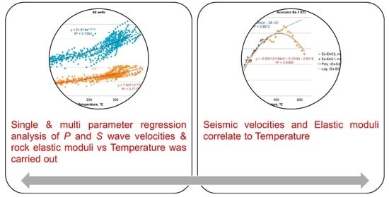
Single regression analysis performed using the 1-D ambient seismic S-wave velocity and elastic modulus profiles as a function of natural state temperature profiles are presented in Figure 7. In Figure 7, the data points corresponding to measured temperatures down to 1800 m depth in well EAC-1 are shown with blue diamonds, while the simulated data points extrapolated down to 3700 m depth in well EAC-2 are shown with orange squares. A logarithmic function with temperature results in the case of measured data points, but a second-order polynomial function results for the simulated extrapolated to depth data points, as S-wave seismic velocity and elastic modulus show a local peak at 2900 m depth around 3 km/s and 22.5 GPa, respectively.

4. Discussion

The analysis has been performed utilizing elastic seismic quantities, which produces results independent of seismic frequency. This is valid for the depths at which this analysis has been performed for Los Humeros (less than 3 km from the surface), but may not be valid for the deepest part of Acoculco, where high temperatures are extrapolated. However, in the deepest part of volcanic geothermal systems and close to the heat source, seismic parameters have typically inelastic behavior, as shown by Poletto et al. [14,25] and Farina et al. [15]. In this case, when inelasticity is included in the analysis, results dependent on the seismic frequency could be expected. We consider that this aspect can be subject to further investigations.

In all graphs, the same correlation trend is followed by seismic velocities and the corresponding elastic moduli, indicating that bulk formation density plays a minor role in the relationship with temperature and that density variability is much smaller than seismic velocity variability.

In Los Humeros, the active and passive seismic results were different in the shallower zone from 1 to 3–4 km depth. This fact, which is still under investigation, can be attributed to the different resolution of the local active and regional passive seismic methods, and/or to the changes that occurred within the reservoir after more than 20 years of exploitation, as the active seismic survey was carried out in 1998, while the passive seismic survey was carried out during 2018–2019.

During this period, huge quantities of fluid mass have been extracted from the Los Humeros reservoir, while only a tiny percentage of this fluid mass was reinjected, resulting in a huge reduction in reservoir (pore) pressure, e.g., by 140 bars in well H-1/H-1D, and an increase in vapor saturation as the fluid boiled out from its initial liquid state [26]. The different correlations with temperature derived could be at least partly attributed to the fact that reservoir temperatures have also changed during the same period, while the same temperature spatial distribution was assumed in this work. Reservoir temperature changes could occur due to a decline in pressure following the boiling point curve, due to recharge from superhot steam from below, and due to inflow of cold reinjected water locally or naturally recharging meteoric water in field boundaries.

As the necessary critical assumptions of multiple linear regression models were not met, the multiple parameter linear regression analysis performed did not yield statistically valid correlation models.

On the other hand, correlations of seismic and elastic parameters with temperature were derived by single parameter linear regression analysis in the vertical direction with R² > 0.95, which were exponential in Los Humeros superhot and logarithmic in Acoculco EGS. However, no such correlation was observed in the horizontal direction. In addition, although the theoretical models of seismic velocities and elastic moduli discussed in the introduction correspond to descending with temperature functions, the correlations observed by analyzing measured data presented in Figure 1, Figure 2, Figure 3, Figure 4 and Figure 5 and Figure 7 correspond to ascending with temperature functions.

This suggests that no direct relation of seismic velocities or elastic moduli with temperature is evident, but an indirect relationship exists among the considered seismic and elastic variables with temperature, possibly due to interdependence on other parameters, such as pressure. Pressure should be the dominant parameter since it is related directly to depth (vertical direction): a rule of thumb in geothermal fields is that confined pressure is lithostatic and pore pressure is hydrostatic, no matter what the physical state of the pore fluid is, e.g., vapor, liquid or two-phase. Other influences in the seismic and elastic parameters could be vapor saturation, porosity, etc., according to the models discussed in the introduction of this paper. In the Los Humeros superhot field, temperature follows the boiling point to depth model; therefore, it is directly related to pressure. In the Acoculco EGS field, temperature increases linearly to depth, and therefore it is also related to pressure, indirectly this time, with depth being the independent parameter.

The common relation of seismic velocities and temperature to pressure explains the strong 1-D correlation between them in the vertical direction and their weaker but still evident overall 3-D correlation. The fact that such a correlation exists, even indirectly, could allow us to predict temperatures at deeper levels, as reliable seismic velocities are derived by inverting seismic data obtained from surface measurements during active or passive seismic surveys, while reliable temperature extrapolation to the depth from measurements at shallow depths is not possible, as there is a cutoff depth beneath which the temperature model derived from shallow measurements is no longer valid. Elastic moduli could also be calculated from seismic velocities, by using bulk formation densities estimated by inverting the gravity field measured at the surface.

Plotting the seismic velocities or elastic moduli with temperature values measured within shallow wells and extrapolating the resulting correlation functions could provide temperature predictions to depth. The fact that a maximum or a local peak value exists at a certain depth in the seismic velocity and elastic moduli fields may allow us to estimate the maximum depth until which the assumed temperature model to depth (boiling point to depth, constant temperature gradient, etc.) is valid. Therefore a more reliable estimate of the deeper reservoir temperature may result, which is the most important parameter for evaluating the feasibility and defining the exploitation plan of the resource. This hypothesis is based on 1-D analysis and may only be valid in the central part of the geothermal resource, as it does not consider the lateral variation in the caldera structure. In addition, this hypothesis needs to be verified in other geothermal fields as well.

5. Proposals for Further Research

As the analysis was performed using only data obtained from sensing-at-surface methods, without direct geophysical calibration at depth, a distributed fiber-optic seismic and temperature sensing system at both surface and downhole is proposed for active-source and passive seismic monitoring, and seismic-while-drilling is considered for reverse vertical seismic profile (RVSP) recording whenever possible for future high-temperature geothermal applications [27].

Two technologies are proposed in the following for the possible utilization of vertical seismic profile (VSP) in superhot geothermal wells. It is well known that the high-temperature conditions, above 250 °C, that exist in Los Humeros wells make it difficult to utilize conventional wireline VSP tools because of the limitations in the electronic and wireline cable technology, which as a standard in non-geothermal conditions can operate at temperatures of the order of 150 °C. This limitation would require the cooling of the well by mud circulation and performing the acquisition in a limited time, with the risk of problems in case of delays, and this operation requires the presence of the drilling rig. In the absence of the rig, this method is problematic. Recently, some logging tool prototypes have been developed and tested in the framework of the DESCRAMBLE H2020 project [28] for the exploitation of supercritical water from deep geothermal resources, with an insulated logging probe allowing downhole measurements to be performed in a well at high pressure and temperatures of the order of 400 °C for six hours.

To extend the applicability of VSP in geothermal wells, we discuss and propose here two alternative approaches to the conventional wireline one. The first one is reverse VSP (RVSP) by seismic while drilling (SWD) using the drilling noise. The method has been known for several years, and recent improvements have been demonstrated. Invoking the reciprocity principle, thanks to the reciprocal (or reverse) geometry with the source at the bit, i.e., the working drill bit itself, and the receivers at the surface, or in other wells (crosswell), the method can also be potentially used at high temperatures of the drilled formation.

The second approach is the use of fiber-optic distributed sensing systems. In this case, the receiver is in the borehole, but it can also be used at the surface, and the sources are at the surface (active seismic sources), while they can also be passive in the subsurface (microseismic sources). This recording technology utilizes the optical signals created by a laser interrogator and transmitted and scattered through the fiber line. This makes it possible to create an array of distributed sensors for acoustic and seismic monitoring (DAS) all along the fiber. Since the system utilized in the well is optical (i.e., the fiber itself), the limitations for high-temperature conditions are very different with respect to those of the electronic systems, e.g., the high temperatures encountered (as 300 °C or more) in deep geothermal wells can be tolerated by the fiber-optic system. Other advantages of DAS are their low cost and their ability to cover a wide area with continuous measurement sampling (e.g., every meter) and time-lapse (4-D) recordings, while the corresponding equipment (fiber and electronics) can be installed permanently within wells or at the surface.

Joint use of both methods and tools, i.e., a permanent distributed acoustic-sensing fiber-optic-sensing system combined with seismic-while-drilling reverse VSP recording when possible, will maximize subsurface imaging information during geothermal resource exploration and exploitation.

6. Conclusions

In the upper 3 km of the Los Humeros superhot geothermal system, subsurface p-wave and S-wave seismic velocities and elastic moduli were correlated to natural state temperatures with ascending convex exponential functions with an overall correlation coefficient R² just above 0.75. Seismic velocities and elastic moduli were derived from inversion of legacy active seismic survey, recent passive seismic monitoring, and ambient seismic noise interferometry, while natural state formation temperatures were estimated from evaluation of temperature logs carried out in the 56 deep geothermal wells drilled in the field, logs provided by courtesy of CFE.

In Los Humeros, although the multiple parameter linear regression analysis performed did not result in any statistically valid correlation models, this was not the case for the single parameter linear regression analysis performed. According to the results of the latter, velocity and moduli correlated to temperature with ascending convex exponential functions in the vertical dimension (R² > 0.95), but did not correlate at all in the horizontal direction (R² close to 0). Considering also that theoretical models suggest descending correlation functions to temperature, we conclude that there should be an indirect dependency on temperature, e.g., through common dependency on a third independent parameter. Pressure should be this parameter, as in hydrothermal fields confined pressure is lithostatic to depth, pore pressure follows the hydrostatic model to depth, and temperature depends on pressure with the boiling point to depth model.

In the Acoculco enhanced geothermal system, the correlation of S-wave seismic velocity derived from ambient seismic noise interferometry to measured natural state temperature profile in the two deep wells drilled in the field yielded an ascending concave function with R² > 0.95. Extrapolation of this function to depth, until the local peak of the seismic velocity or modulus profile, could provide a hint of the maximum temperature expected in the deep part of the system, as indicated by the temperature extrapolation to depth beneath the well bottom until this point, assuming a conduction heat flow model, which is valid for EGS where no fluid flow is expected.

One limitation concerning the accuracy of the methodology adopted was the coarse network of seismic sensors at the surface. A more refined time-lapse subsurface distribution of seismic velocities and elastic moduli can be obtained by using a permanent network of distributed acoustic sensing (DAS) fiber optic tools, which will also allow seismic-while-drilling reverse VSP recordings whenever a new well is drilled.