Comparison among Methods and Statistical Software Packages to Analyze Germplasm Genetic Diversity by Means of Codominant Markers

Abstract

Co-dominant markers’ data are often analysed as if they were dominant markers, an over-simplification that may be misleading. Addressing this, the present paper aims to provide a practical guide to the analysis of co-dominant data and selection of suitable software. An overview is provided of the computational methods and basic principles necessary for statistical analyses of co-dominant molecular markers to determine genetic diversity and molecular characterization of germplasm collections. The Hardy–Weinberg principle is at the base of statistical methods to determine genetic distance, genetic diversity, and its distribution among and within populations. Six statistical software packages named GenAlEx, GDA, Power Marker, Cervus, Arlequin, and Structure are compared and contrasted. The different software packages were selected based on: (i) The ability to analyze co-dominant data, (ii) open access software, (iii) ease of downloading, and (iv) ease of running using a Microsoft Window interface. The software packages are compared analyzing the same dataset. Differences among parameters are discussed together with the comments on some of the software outputs.

1. Introduction

Genetic diversity of germplasm is assessed by collecting key information, especially: (i) Allele number per locus; (ii) genotype number per locus; (iii) gene diversity; (iv) PIC (polymorphism information content) values; (v) observed and expected heterozygosity; (vi) partition of the diversity into its components within and between populations; and (vii) the genetic distance among the analyzed populations. The analyses are usually performed using a variety of molecular markers grouped into two categories: Co-dominant markers, such as SSR (single sequence repeat) and SNP (single nucleotide polymorphism), which are able to identify the allelic situation at each locus, and dominant markers, such as ISSR (inter simple sequence repeats), RAPD (random amplified polymorphic DNA), and AFLP (amplified fragment length polymorphism), which usually have a multi-band pattern and are unable to recognize allelic variants [1]. The latter produce a series of bands with unknown relationships (i.e., could be allelic variants of the same genes or mark different genome regions). Hence, without knowing the allelic situation, each band is recorded as a locus with two possible alleles’ band presence (scored as 1) or band absence (scored as 0) and the relative 0/1 matrix is used in statistical analyses. The papers reviewed here comprise data based on co-dominant markers that were often wrongly recorded as the presence/absence of possible bands, leading to a loss of information on allelic variance and the presence of heterozygosity (observed heterozygosity, Ho).

The present paper offers a short and simple guide to the principles that form the base of the most common analyses. It focuses on some of the most widely-used computer programs in population genetics, run under Windows, to highlight the advantages and disadvantages of the various software packages, thus facilitating appropriate selection and use.

1.1. Hardy–Weinberg Principle

Most of the statistical computations use parameters based on the Hardy–Weinberg principle [2,3]. Here, the basis of the principle and its applications are highlighted. As it is widely known, the Hardy–Weinberg principle considers the genetic and genotype frequency for a single locus in a population and states: “allele and genotype frequencies in a population will remain constant from generation to generation in the absence of other evolutionary influences”. These potential evolutionary forces include: (i) Migration, (ii) mutation, (iii) selection, (iv) population size sufficient to avoid drift, and (v) random mating. Unfortunately, this definition of the Hardy–Weinberg does not sufficiently focus on other important consequences of the principle such as: “if a population is in equilibrium it is possible to compute the allele frequencies knowing the genotype frequencies and vice-versa by the formula of binomial square development i.e., (p + q)² = p² + q² + 2pq = 1”, where p² is the frequency of the AA genotype, q² indicates the aa genotype frequency, 2pq the Aa genotype frequency, p the A allele frequency, and q the a allele frequency. This equation is true only for a population in the Hardy–Weinberg equilibrium where it is possible to compute allele frequencies from knowing the genotype frequencies and vice versa. The above is if only two alleles, A and a, are possible for that locus. If, instead, three alleles may occur at a locus, the formula would be a trinomial square development ((p + q + r)² = p² + q² + r² + 2pq + 2pr + 2qr = 1) and so on for higher numbers of alleles. It should be noted that the square terms (i.e., p² + q² + r², etc.) are homozygote frequencies while the others (i.e., 2pq + 2pr + 2qr, etc.) are heterozygotes. Considering several alleles, I, with a frequency, p_i, the homozygote frequency is Ʃp_i² and heterozygote frequency can be calculated as the complementary difference from the homozygote frequency (i.e., 2pq = 1 − (p² + q²) or 1 − Ʃp_i²).

1.2. Genetic Diversity

The gene diversity index is calculated for each locus and population according to Nei [4], utilizing the Hardy–Weinberg formula, $He=1-{{\displaystyle \sum }}_{i=1}^n{p}_i^2$, hereafter simplified as He = 1 − Ʃp_i², which is the heterozygosity expected if the population is in Hardy–Weinberg equilibrium. In analogy, the genetic identity (J) is Ʃp_i² (homozygotes). However, since He could be computed for all populations, including non-random mating systems (e.g., autogamus, which, by definition, will not in Hardy–Weinberg equilibrium being a pure line with homozygosity for all loci), the terminology for He is thus gene diversity, rather than expected heterozygosity.

In a small population, the alleles per locus can be skewed, especially when compared to large populations [5]. Unbiased heterozygosity is as for the above-mentioned heterozygosity multiplied by the factor, 2n/(2n − 1) [6]. As a result, the larger the population, the lower are the differences between the biased and unbiased expected heterozygosity. This detail is often not sufficiently elaborated upon in the literature, as many papers do not mention whether unbiased or biased He is used.

The variability between and within populations can be calculated according to Nei [4] by taking into account different allele frequencies in whole populations or only in subpopulations. The nomenclature used is: H_T for total observed diversity; H_S for within-population diversity; and D_ST for the between-population diversity, with H_T = H_S + D_ST.

Similarly, the Wright’s fixation indices, F_IS, F_ST, and F_IT [7], are often used, also the F-statistics are based on the expected level of heterozygosity. The measures describe the different levels of population structures, such as variance of allele frequencies within populations (F_IS), variance of allele frequencies between populations (F_ST), and an inbreeding coefficient of an individual relative to the total population (F_IT), all of which are related to heterozygosity at various levels of population structure. The terms mentioned above are represented by the formula, 1 − F_IT = 1 − F_IS + 1 − F_ST, where I is the individual, S the subpopulation, and T the total population. F_IT thus refers to the individual in comparison with the total, F_IS is the individual in comparison with the subpopulation, and F_ST is the subpopulation in comparison with the total. As shown in Figure 1, total F, indicated by F_IT, can be partitioned into F_IS (or f) and F_ST (or θ).

F_ST can be calculated using the formula: F_ST = (H_T − H_S)/H_T, where H_T is the proportion of the heterozygotes in the total population and H_S the average proportion of heterozygotes in subpopulations.

In a series of loci, l, in n populations and using the complementary sum of allele frequency (1 − Ʃp_i²), different figures can be obtained. In particular:

• For each locus and each population, He = (1 − Ʃp_i(lg)²), where p_i(lg) is the ith allele frequency of the lth locus in the gth population.
• The average of the above He over populations gives the genetic diversity within a population for each locus, while the average of all the loci within a population diversity gives H_S. The formula can thus be written as: H_S = (Ʃ_l(Ʃ_g(1 − Ʃ_pi(lg)²)/_g)/_l), where (1 − Ʃp_i(lg)²) indicates the expected heterozygosity for each locus in each population, g indicates the number of populations, and l the loci number.
• The total genetic diversity, H_T, is calculated using the allele frequency, p_i(l), for each locus over all populations and calculating the mean over loci: H_T = Ʃ(1 − Ʃ_pi(l)²)/_l).
• The between population component of diversity is calculated using the formula: D_ST = H_T − H_S.
• The between population component may also be expressed in relation to the total genetic diversity (for each locus and overall loci) as G_ST = H_T/D_ST [4].

Table 1. Allelic situation and computation of the genetic parameters in three populations analyzed using two markers where each one has three possible alleles; adapted from Turpeinen et al. [8].

Locus\Pop	Pop1	Pop2	Pop3				Mean
Locus 1		10	10
167	0.00	0	0				0.00
168	0.50	0	0.9				0.47
172	0.50	1	0.1				0.53
He	0.50	0.00	0.18	HS	0.23	HT	0.50
Locus 2
218	0.50	0.00	0.10				0.20
221	0.10	1.00	0.10				0.40
224	0.40	0.00	0.80				0.40
He	0.58	0.00	0.34	HS	0.31	HT	0.64
	HT	HS	DST	GST
Locus 1	0.50	0.23	0.27	0.54
Locus 2	0.64	0.31	0.33	0.52
Mean	0.57	0.27	0.30	0.53

shows an example extracted from Turpeinen et al. [8], where different parameters for three populations were analyzed using two markers. The H_T for each locus corresponds to the polymorphic information content (PIC) of that locus, which in other words, consists in the capacity of that locus (or better a marker) to assess polymorphism and diversity. Botstein et al. [9] proposed an adjustment of this value as:

$$PIC=1-{\displaystyle \sum }_{i=1}^n{p}_i^2-{\displaystyle \sum }_{i=1}^{n-1}{\displaystyle \sum }_{j=i+1}^{n}2p_i^2{p}_j^2$$

where p_i and p_j are the population frequency of the ith and jth alleles. The PIC proposed by Botstein and colleagues [9] subtracts from the He value an additional probability (ƩƩ2p_i²p_j²) due to the fact that linked individuals do not add information to the overall variation.

1.3. Genetic Distance

Genetic diversity (He) and genetic identity (J or Ho) are also used to estimate the genetic distance within and between populations, since two populations with high identity in their genes are closer than two with high diversity. If J_x = Ʃp_xi² is the probability of identity in population x with p_xi the frequency of the i-th allele and J_y = Ʃp_yi² is the probability of identity in population y, the probability of identity in both populations is J_xy = Ʃp_xip_yi as described by Nei [10,11]. The probability of identity in population x for all normalized loci is I = J_xy/√(J_xJ_y) and, in turn, the genetic distance is D = −LnI = −Ln (J_xy/√(J_xJ_y)). In a small sample set with many loci, any biases can be corrected using Ď = −Ln G_xy/√(G_xG_y), where G_x and G_y are (2n_xJ_x − 1)/(2n_x − 1) and (2n_yJ_y − 1)/(2n_y − 1) over the l loci studied, respectively, and G_xy = J_xy [12]. In this case, Ď could be negative, due to sampling errors, and hence considered as zero.

Various software packages can be used to calculate the above-mentioned parameters; they often use different parameters and have their own advantages and disadvantages. In general, for the analyses of genetic diversity, characteristics required in statistical software are: (i) Precision (no bugs), accuracy, and reproducibility; (ii) user friendliness (e.g., do not need command line scripts); (iii) clear output in terms of graphical options; and (iv) that it is open access. This paper compares some software packages that run using Microsoft Windows, which are generally used to calculate population genetic analyses. The software packages assessed are:

• GenAlEx [13], http://biology-assets.anu.edu.au/GenAlEx/Welcome.html
• GDA [14], http://en.bio-soft.net/dna/gda.html or now at https://phylogeny.uconn.edu/software/
• Popogene [15], https://sites.ualberta.ca/~fyeh/popgene.html
• Power Market [16], http://statgen.ncsu.edu/powermarker/index.html
• Cervus [17], www.fieldgenetics.com
• Arlequin [18], http://cmpg.unibe.ch/software/arlequin3/
• Structure v 2.3 [19], http://web.stanford.edu/group/pritchardlab/structure.html

Software description and comparison is carried out using examples of data obtained with SSR markers (hence, co-dominant) on nine durum wheat populations from three Ethiopian regions as described by Mondini et al. [20]. For the purpose of this assessment, the analyses of 10 genotypes per population are reported.

2. Data Input

One of the first issues is the data format required as the various software packages use different data-file formats. A difference of a single comma or space can make the data unreadable or misclassified. As a result, it often takes more time to organize the data into the correct format than to run the analysis itself. Some programs may offer the possibility of importing/exporting data from/to other formats, thereby avoiding reformatting data manually and making it easier and faster to analyze a given data set with different programs. This is of particular importance where the data set may require the use of more than one application and/or analyses offered by different software packages.

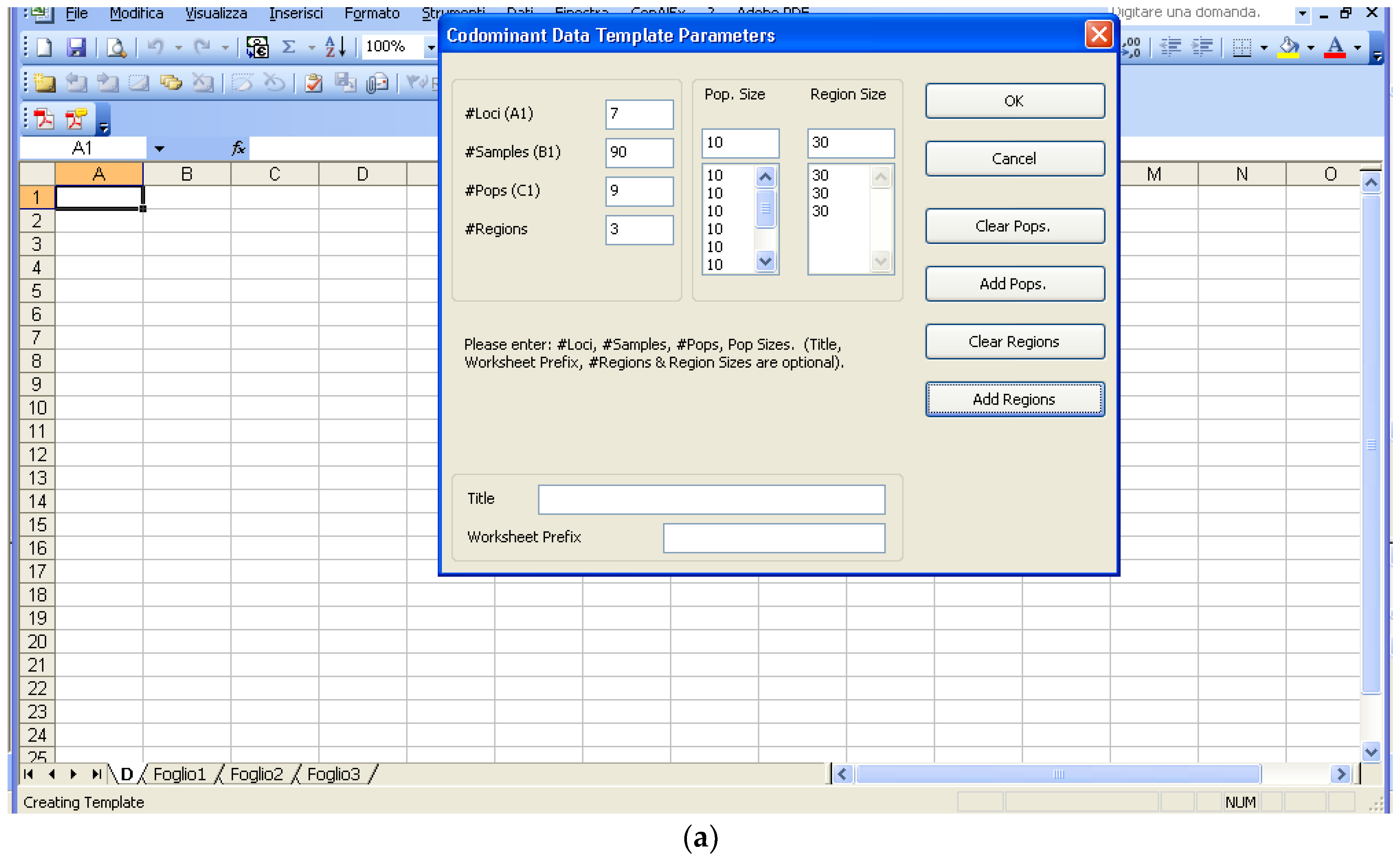
The amplicons generated from markers are distinguished by submarine gel electrophoresis or a capillary in a sequencer; in the later cases, the results, as alleles call, can be exported from the sequencer into a Microsoft Excel file. Excel seems to be the easiest and most universal way to insert data. As such, GenAlEx [13], which is an Excel macro rather than a full software package, is first to be considered. GenAlEx software, as its 6.5 version [21], can be downloaded from http://biology.anu.edu.au/GenAlEx/Download.html and has a template function for co-dominant, binary, and haploid data, creating a framework on which data insertion can be easily carried out starting from the cell C4. After the data are inserted, they can be analyzed directly by GenAlEx or alternatively be exported to other formats specific to other commonly used statistical software. The present example entails seven loci, 90 samples, nine populations, and three regions, which are indicated in the template (Figure 2a).

The results are stored in an Excel sheet where the loci and the populations are indicated with consecutive numbering; it is possible, however, to change these to the correct locus and population names. Being co-dominant data, each locus will have two columns for the two alleles (Figure 2b). GenAlEx can also be used to import or export data from or to other software packages, although it is very important to pay attention to the codes used by the different software to indicate missing data. For example, the alleles can be easily named with their molecular weight in bp, however, the null allele (which is not missing data) could be named as zero, but zero is considered missing for some software, such as GenAlEx, when co-dominance is the option selected. In these cases, it is important to rename the null allele, for example, by substituting zero with 1.

3. Data Analysis

The same data was then analyzed using various software packages and the various outputs compared and reported here.

3.1. GenAlEx

GenAlEx is available at http://biology-assets.anu.edu.au/GenAlEx/Welcome.html, as mentioned above. It is an Excel macro used for statistical genetic analysis, so the user should be registered for an Office package which is not open source. By using the “Frequency…” option, it is possible to compute allele frequency, heterozygosity, F-stat, and polymorphism by population and by locus, some genetic distances (i.e., Nei distance, Nei unbiased distance, pairwise F_ST) together with some graphic options (Figure 3).

One of the positive aspects of GenAlEx is that the different output-sheets display the base of the statistic used. There are also options for graphics (i.e., Allele Frequencies by Population with Graph over Loci or Graphs by Population and Locus) that provide a quick overview of allele distribution among populations. The most important outputs are in the sheets “HFP” and “HFL”, where the different statistical parameters by locus (

Table 2. GenAlEx output of the data in Figure 2 per locus. Sheet HFL.

		WMC24	BARC213	BARC8	wms124	WMC177	WMC170	CFA2278	Mean	SE
N	Mean	9.333	8.667	9.889	9.556	10.000	9.667	9.889
	SE	0.333	0.236	0.111	0.242	0.000	0.167	0.111
Na	Mean	3.222	4.444	3.222	1.667	3.444	4.000	1.444
	SE	0.547	0.475	0.401	0.289	0.475	0.408	0.176
Ne	Mean	2.167	3.374	1.949	1.424	2.106	2.742	1.176
	SE	0.287	0.411	0.322	0.212	0.308	0.292	0.100
I	Mean	0.825	1.266	0.747	0.321	0.829	1.099	0.183
	SE	0.154	0.131	0.145	0.140	0.158	0.132	0.081
Ho	Mean	0.289	0.143	0.035	0.000	0.122	0.117	0.000
	SE	0.084	0.032	0.017	0.000	0.057	0.029	0.000
He	Mean	0.466	0.657	0.395	0.198	0.436	0.585	0.113
	SE	0.074	0.051	0.075	0.087	0.079	0.065	0.054
uHe	Mean	0.493	0.698	0.416	0.209	0.459	0.617	0.119
	SE	0.078	0.054	0.079	0.092	0.084	0.068	0.057
F	Mean	0.426	0.803	0.887	1.000	0.693	0.726	1.000
	SE	0.119	0.045	0.054	0.000	0.130	0.106	0.000
Pops	FIS	0.381	0.783	0.913	1.000	0.720	0.799	1.000
	FIT	0.566	0.838	0.954	1.000	0.767	0.853	1.000	0.854	0.058
	FST	0.300	0.253	0.471	0.308	0.167	0.269	0.210	0.282	0.037
	Nm	0.584	0.739	0.281	0.562	1.246	0.680	0.941	0.719	0.116

) and/or by populations (

Table 3. GenAlEx output of the data in Figure 2 per population. Sheet HFP.

Mean and SE over Loci for Each Pop
Population		N	Na	Ne	I	Ho	He	uHe	F
Pop1	Mean	9.000	3.286	2.400	0.921	0.068	0.520	0.551	0.857
	SE	0.436	0.421	0.348	0.147	0.025	0.077	0.081	0.059
Pop2	Mean	9.714	3.286	2.268	0.853	0.073	0.475	0.501	0.750
	SE	0.184	0.565	0.412	0.174	0.029	0.083	0.088	0.142
Pop3	Mean	9.857	2.286	1.535	0.450	0.057	0.249	0.262	0.832
	SE	0.143	0.522	0.254	0.186	0.043	0.103	0.108	0.090
Pop4	Mean	9.571	2.714	1.697	0.622	0.089	0.347	0.367	0.783
	SE	0.297	0.360	0.246	0.138	0.041	0.074	0.079	0.106
Pop5	Mean	9.714	4.286	2.934	1.088	0.221	0.541	0.571	0.635
	SE	0.184	0.778	0.509	0.245	0.097	0.119	0.125	0.143
Pop6	Mean	9.714	3.571	2.461	0.900	0.164	0.477	0.504	0.694
	SE	0.286	0.719	0.550	0.217	0.096	0.101	0.107	0.161
Pop7	Mean	9.286	2.429	1.733	0.539	0.122	0.303	0.320	0.547
	SE	0.286	0.528	0.358	0.195	0.068	0.105	0.111	0.171
Pop8	Mean	9.429	2.857	1.932	0.687	0.066	0.370	0.392	0.840
	SE	0.297	0.595	0.359	0.209	0.036	0.108	0.114	0.064
Pop9	Mean	9.857	2.857	2.245	0.716	0.046	0.383	0.404	0.886
	SE	0.143	0.705	0.481	0.262	0.033	0.138	0.145	0.056
Grand Mean and SE over Loci and Pops
		N	Na	Ne	I	Ho	He	uHe	F
Total	Mean	9.571	3.063	2.134	0.753	0.101	0.407	0.430	0.755
	SE	0.090	0.198	0.136	0.067	0.019	0.034	0.036	0.039
Population	%P
Pop1	100.00%
Pop2	100.00%
Pop3	57.14%
Pop4	100.00%
Pop5	85.71%
Pop6	85.71%
Pop7	71.43%
Pop8	71.43%
Pop9	57.14%
Mean	80.95%
SE	5.83%

) are provided. The parameters are:

• N: (number of genotypes);
• Na: (No. of Different Alleles);
• Ne: (No. of Effective Alleles = 1/(Σp_i²));
• I: (Shannon’s Information Index = −1 × Σ(p_i × Ln(p_i)));
• Ho: (Observed Heterozygosity = No. of Hets/N);
• He: (Expected Heterozygosity = 1 − Σp_i²);
• uHe: (Unbiased Expected Heterozygosity = (2N/(2N − 1)) × He);
• F: (Fixation Index = (He − Ho)/He = 1 − (Ho/He));
• Fis: (Mean He − Mean Ho)/Mean He);
• Fit: (H_T − Mean Ho)/H_T), F_ST (H_T − Mean He)/H_T);
• Nm: ([(1/Fst) − 1]/4);
• H_T: Total Expected Heterozygosity = 1 − Σtp_i².

Where tp_i is the frequency of the ith allele for the total and Σtp_i² is the sum of the squared total allele frequencies.

The three levels of the fixation indexes (F_IS, F_IT, F_ST) are computed per locus and not per population as in other programs, such as Arlequin (see below).

The output of different genetic distances, such as the Nei’s distance, Nei’s unbiased distance, and pairwise F_ST, are reported in

Table 4. Computation of different parameters of distance between populations. Sheets NeiP, uNeiP, and F_STP. (A) Nei’s genetic distance [10]; (B) Pairwise Population Matrix of Nei’s Unbiased Genetic Distance; (C) Pairwise Population F_ST Values.

(A)
Population	Pop1	Pop2	Pop3	Pop4	Pop5	Pop6	Pop7	Pop8	Pop9
Pop2	0.406	0.000
Pop3	0.569	0.234	0.000
Pop4	0.602	0.224	0.032	0.000
Pop5	0.615	0.401	0.236	0.222	0.000
Pop6	0.513	0.250	0.120	0.127	0.249	0.000
Pop7	0.947	0.619	0.598	0.577	0.445	0.495	0.000
Pop8	0.624	0.540	0.398	0.376	0.163	0.416	0.579	0.000
Pop9	0.392	0.386	0.336	0.290	0.237	0.374	0.619	0.251	0.000
(B)
Population	Pop1	Pop2	Pop3	Pop4	Pop5	Pop6	Pop7	Pop8	Pop9
Pop2	0.347	0.000
Pop3	0.527	0.200	0.000
Pop4	0.553	0.183	0.008	0.000
Pop5	0.548	0.342	0.194	0.173	0.000
Pop6	0.453	0.199	0.085	0.085	0.189	0.000
Pop7	0.901	0.582	0.577	0.549	0.399	0.456	0.000
Pop8	0.573	0.497	0.372	0.343	0.112	0.373	0.550	0.000
Pop9	0.341	0.344	0.310	0.258	0.186	0.330	0.589	0.217	0.000
(C)
Population	Pop1	Pop2	Pop3	Pop4	Pop5	Pop6	Pop7	Pop8	Pop9
Pop2	0.142	0.000
Pop3	0.248	0.140	0.000
Pop4	0.214	0.105	0.044	0.000
Pop5	0.162	0.139	0.141	0.096	0.000
Pop6	0.157	0.108	0.105	0.076	0.104	0.000
Pop7	0.279	0.246	0.364	0.241	0.181	0.234	0.000
Pop8	0.215	0.211	0.257	0.163	0.080	0.187	0.290	0.000
Pop9	0.179	0.197	0.234	0.143	0.110	0.190	0.308	0.152	0.000

.

GenAlEx can calculate the molecular analysis of variance (AMOVA), which partitions genetic variability into different components (

Table 5. AMOVA (analyses of molecular variance) output of GenAlEx.

Source	df	SS	MS	Est. Var.	%
Among Regions	2	27.828	13.914	0.033	2%
Among Pops	6	71.567	11.928	0.515	24%
Within Pops	171	277.550	1.623	1.623	75%
Total	179	376.944		2.171	100%

), including, or not, the individual level.

3.2. GDA

GDA can be downloaded at http://en.bio-soft.net/dna/gda.html or now at https://phylogeny.uconn.edu/software/. Data can be exported from GenAlEx to GDA, but it is necessary to manually change the file extension. A useful tool of GDA is the possibility of easily re-running the analysis excluding/including loci and/or populations.

The descriptive statistics offered by GDA are: (i) Number of alleles per population (A), (Na in GenAlEx); (ii) polymorphic alleles per locus, (not available in GenAlex); (iii) expected (He); and (iv) observed (Ho) heterozygosity. Observed heterozygosity is in line with GenAlEx output, while the He is here the unbiased expected heterozygosity (uHe in GenAlEx). GDA outputs per population and per locus are reported in

Table 6. Descriptive statistics output of GDA per population (A) and per locus (B). Where n is the number of observations, P the polymorphism, A the alleles number, Ap the polymorphic alleles number, He the expected heterozygosity, and Ho the observed heterozygosity.

(A) output per population
Population	n	P	A	Ap	He	Ho
Pop1	9.00	1.00	3.29	3.29	0.55	0.07
Pop2	9.71	1.00	3.29	3.29	0.50	0.07
Pop3	9.86	0.57	2.29	3.25	0.26	0.06
Pop4	9.57	1.00	2.71	2.71	0.37	0.09
Pop5	9.71	0.86	4.29	4.83	0.57	0.22
Pop6	9.71	0.86	3.57	4.00	0.50	0.16
Pop7	9.29	0.71	2.43	3.00	0.32	0.12
Pop8	9.43	0.71	2.86	3.60	0.39	0.07
Pop9	9.86	0.57	2.86	4.25	0.40	0.05
Mean	9.57	0.81	3.06	3.58	0.43	0.10
(B) output per locus
Locus	n	P	A	Ap	He	Ho
WMC24	84.00	1.00	8.00	8.00	0.66	0.30
BARC213	78.00	1.00	12.00	12.00	0.89	0.14
BARC8	89.00	1.00	12.00	12.00	0.75	0.03
wms124	86.00	1.00	3.00	3.00	0.29	0.00
WMC177	90.00	1.00	10.00	10.00	0.53	0.12
WMC170	87.00	1.00	11.00	11.00	0.80	0.11
CFA2278	89.00	1.00	2.00	2.00	0.15	0.00
All	86.14	1.00	8.29	8.29	0.58	0.10

.

Table 7. Private alleles (i.e., allele present in a single population).

Locus	Allele	Frequency	Found in
WMC24	171	0.050	Pop5
WMC24	153	0.050	Pop5
WMC24	169	0.150	Pop5
BARC213	204	0.200	Pop6
BARC213	224	0.050	Pop4
BARC8	248	0.100	Pop8
BARC8	242	0.100	Pop7
BARC8	272	0.050	Pop2
BARC8	274	0.050	Pop1
WMC177	246	0.300	Pop9
WMC177	212	0.100	Pop8
WMC177	204	0.100	Pop7
WMC177	220	0.150	Pop5
WMC177	222	0.050	Pop5
WMC170	214	0.100	Pop8
WMC170	220	0.100	Pop8
WMC170	248	0.050	Pop6
WMC170	230	0.050	Pop4

shows the private alleles, another useful option present in GDA. In

Table 8. Genetic distances computed by GDA. Above diagonal Nei (1978) [12] distance; below diagonal Nei (1972) [10] distance.

	Pop1	Pop2	Pop3	Pop4	Pop5	Pop6	Pop7	Pop8	Pop9
Pop1		0.35	0.53	0.55	0.55	0.45	0.90	0.57	0.34
Pop2	0.41		0.20	0.18	0.34	0.20	0.58	0.50	0.34
Pop3	0.57	0.23		0.01	0.19	0.09	0.58	0.37	0.31
Pop4	0.60	0.22	0.03		0.17	0.09	0.55	0.34	0.26
Pop5	0.62	0.40	0.24	0.22		0.19	0.40	0.11	0.19
Pop6	0.51	0.25	0.12	0.13	0.25		0.46	0.37	0.33
Pop7	0.95	0.62	0.60	0.58	0.45	0.49		0.55	0.59
Pop8	0.62	0.54	0.40	0.38	0.16	0.42	0.58		0.22
Pop9	0.39	0.39	0.34	0.29	0.24	0.37	0.62	0.25

, genetic distances computed in agreement with Nei (1972) [10] and Nei (1978) [12] are shown; the first is the unbiased genetic distance of GenAlEx, while the second is equal to the genetic distance reported in GenAlEx.

Based on Nei’s genetic distance computed in Table 6, GDA builds up a dendrogram with the UPGMA (Unweighted Pair Group Method with Arithmetic Mean) methodology (Figure 4).

The graphic output is as a text file. To improve the options for the quality of graphs, it is necessary to use other software, such as TreeView [22]. The graphic quality and options are not considered here as it is the ability of the statistic software to export the dendrogram codes to be then used in the graphical software that is of prime importance.

3.3. Popgene

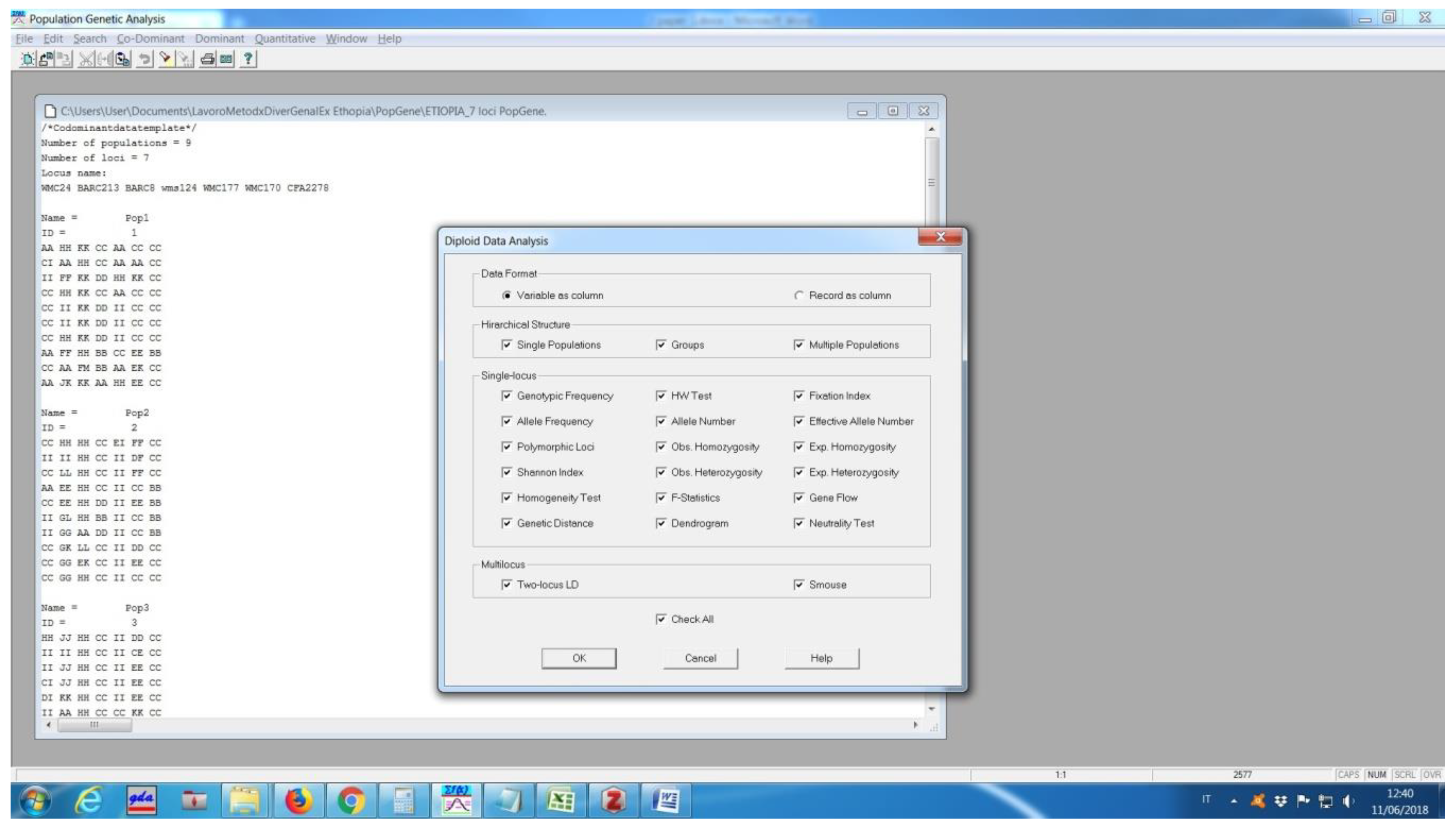
Popgene offers two versions for either 32 or 16 bit Windows operating environments, and can be downloaded at https://sites.ualberta.ca/~fyeh/popgene.html. It immediately divided the analysis depending on whether it deals with dominant or codominant markers. For diploid data, it performs a genotypic frequency, HW test (not commonly found in other packages), fixation index, allele frequency, allele number, effective allele number, polymorphic loci, observed and expected homozygosity and heterozygosity, Shannon index, homogeneity test, F-statistics (F_IT, F_ST, F_IS), gene flow, and genetic distance (following Nei 1972 [10] and Nei 1978 [6]). It also produces a dendrogram using UPGMA of the Nei’s distance, neutrality test, and the linkage disequilibrium (LD) between two loci. In the cases of several alleles per locus, the required input is not straightforward, based on the Mendelian convention (Figure 5), i.e., providing a letter for each allele, but it is possible to export the Popgene format from GenAlEx. However, a significant disadvantage is that it assigns the same letter to alleles from different loci, as if they were the same allele. This creates confusions and errors especially when reading the tables of “Allele Frequency”.

3.4. Power Marker

Power Marker, like GDA, was developed at the North Carolina State University and uses as a reference the Genetic Data Analysis by Weir [23]. The original download source for Power Markers, http://www.powermarker.net/ [16], seems to be expired, however, the program and the manual can be found at http://statgen.ncsu.edu/powermarker/index.html.

Data input is very easy, entering the allelic phase separated by space, tab, and/or commas. It is possible to indicate up to three category levels. In this example, we used: Genotype, populations, and regions. The program is suitable for microsatellite data; however, it also works with haplotypes. The data can be reduced by a sub-selection of genotypes or markers based on particular parameters, such as the level of missing data, heterozygosity, or diversity. Outputs have their own format, which can be easily converted into Excel files. A very useful tool is the internal link with the TreeView [24] graphic program (http://taxonomy.zoology.gla.ac.uk/rod/treeview.html) used to display genotype relationships (Trees) with good graphical resolution. However, to use this function, the user must also install the TreeView program.

The summary table (Figure 6) illustrates information, such as: (i) Allele frequency, (ii) genotype number, (iii) number of observations, (iv) allele, (v) gene diversity, (vi) heterozygosity, and (vii) PIC. Number of observations, allele, gene diversity, heterozygosity, and PIC are equivalent to the values reported in GDA, respectively, as n, A, He, and Ho. In Power Marker, the expected heterozygosity (which is not unbiased expected heterozygosity as in GDA) is named “gene diversity”. It should be noted that the PIC values are here computed according to Botstein et al. [9]. The main disadvantage of Power Marker is that outputs always refer to the markers rather than to the population as per GDA. To show values per population, it is necessary to create a subset of data where only one population is considered each time. Another disadvantage is that the output does not report the options chosen, so naming the folders with self-explaining labels is an imperative.

After the user has computed the allele frequency by using the “phylogeny” option, it is possible to calculate the frequency based distance utilizing several methods. The only equivalent method to the other software in this paper is Nei’s genetic distance 1972 [10]. In addition, Power Maker can compute the pairwise linkage disequilibrium, where the output is displayed for each marker in the order they were inserted in the data file (Figure 7). Therefore, it is crucial that the marker results be entered in the “right” order, which is important only if a genetic map with marker positions along the chromosomes is available.

3.5. Cervus

Cervus is primarily designed for the assignment of parents to their offspring using genetic markers. Nevertheless, it is sometimes used for genetic analysis. It is available for download at www.fieldgenetics.com. The input data sheet is not as user-friendly as some of the other programs, but this can be converted from GenePop, which in turn can be converted from GenAlEx.

It calculates the PIC value as per Botstein et al. [9] and He is unbiased. In crossed populations, Cervus computes the average non-exclusion probability for a series of related genotypes, such as the first and second parent, parent pair, identity, and sib identity (

Table 9. Cervus output reporting the number of alleles per locus (k), number of individuals (N), observed (Hobs) and expected (Hexp) heterozygosity, PIC, combined non-exclusion probability for first parent (NE-1P), second parent (NE-2P), parent pair (NE-PP), identity (NE-I) and sib identity (NE-SI), the Hardy–Weinberg equilibrium significance (HW), and the F test (F).

Locus	k	N	HObs	HExp	PIC	NE-1P	NE-2P	NE-PP	NE-I	NE-SI	HW	F(Null)
WMC24	8	84	0.298	0.663	0.615	0.748	0.575	0.387	0.160	0.460	***	+0.3786
BARC213	12	78	0.141	0.886	0.868	0.391	0.242	0.090	0.026	0.317	ND	+0.7244
BARC8	12	89	0.034	0.754	0.727	0.620	0.435	0.230	0.086	0.397	***	+0.9145
wms124	3	86	0.000	0.285	0.261	0.960	0.858	0.754	0.536	0.742	ND	+0.9766
WMC177	10	90	0.122	0.527	0.508	0.835	0.655	0.448	0.243	0.549	***	+0.6174
WMC170	11	87	0.115	0.804	0.772	0.565	0.388	0.204	0.067	0.367	***	+0.7509
CFA2278	2	89	0.000	0.146	0.134	0.989	0.933	0.879	0.742	0.863	ND	+0.8551
Mean	8.29			0.580	0.555	0.081	0.012	0.000	0.000	0.007

ND = Non significance; *** = Significance (with Bonferroni correction).

). Moreover, it also tests Hardy–Weinberg equilibrium. The program is particularly useful for animal population genetics.

3.6. Arlequin

Arlequin, available at http://cmpg.unibe.ch/software/arlequin3/, produces output displayed in a browser page, and thus is not ideal for conversion into a word document. On the other hand, the particular computation run by Arlequin is AMOVA (analyses of molecular variance) as described by Excoffier et al. [25]. It considers haplotype, and with 90 genotypes, the total degree of freedom is 179 [(90 × 2) − 1] = 2N − 1 (

Table 10. AMOVA (analyses of molecular variance) output of Arlequin.

Source of Variation	d.f.	Sum of Squares	Variance Components	Percentage of Variation	Expected Mean Square
Among Region	2 (R − 1)	27.828	0.03310 Va	1.52	Nσ2a + 2σ2b+ σ2c
Among Populations within Region	6 (P − R)	71.567	0.51523 Vb	23.73	2σ2b + σ2c
Within Populations	171 (2N − P)	277.550	1.62310 Vc	74.75	σ2c
Total	179 (2N − 1)	376.944	2.17144		σ2T

Where: σ²_a = F_ct σ²_T, σ²_b = (F_ST − F_CT) σ²_T, σ²_c = (1 − F_st) σ²_T, F_ST = (σ²_a + σ²_b)/σ²_T, F_SC = σ²_b/(σ²_b + σ²_c), F_CT = σ²_a/σ²_T, F_ST = 0.252 = F_IT, F_SC = 0.240 = F_IS, and F_CT = 0.015 = F_ST.

). The AMOVA output is very similar to the GenAlEx one (Table 5).

He and Ho are reported for each locus within each population and produce the same average outcome as the GDA software. Linkage disequilibrium, where the deviation from random association between alleles at different loci [26], expressed as D = p_ij − p_ip_j, is a potentially useful additional feature of Arlequin. However, although the instruction manual asserts the computation of the linkage disequilibrium coefficient (D) is possible, this seems not to be true. On the contrary, significance is reported as the P values of χ² with 1000 permutations. Moreover, the number of loci linked to each locus for each population analyzed is provided. Unfortunately, even when the locus name is inserted, it is not reflected in the output, where the loci are simply numbered starting at zero. Similarly, the populations are numbered as pop1#, pop2#, pop3#, etc. rather than using the given name. This could easily lead to mistakes and confusion. In addition, there are sometimes discrepancies between the data saved in the browser output file and that saved as an xls file.

3.7. Structure

Structure software [19] is available for downloaded at http://web.stanford.edu/group/pritchardlab/structure.html. Preparation of the data file in order to run Structure presents some problems. Conversion from GenAlEx is not straightforward since (i) an extra space is required at the end of the second row to allow the program to read the last number, and (ii) population names are not converted automatically. Moreover, particular care must be taken when dealing with missing data and their code, for doing so differs from other software packages (in Structure, “−9” is used as default, but it is possible to set it differently). However, with suitable modification, it is easy to convert files directly from Excel by saving it as a text file.

In Structure, the analysis should be set in agreement with the populations’ information and the procedures used in the population sampling. Useful information to assist clustering includes three possible options: (i) Considering individuals with or without common ancestry, (ii) with or without use of sampling locations, and (iii) to set the allele frequencies as either independent or dependent in each population.

Fundamentally, Structure performs a K-mean cluster analyses [27]. As with all K-mean cluster methods, in Structure, the analysis should be performed trying different values for the number of clusters (K). Clearly, some logical pre-cluster division can be argued in agreement with the data typologies, number of populations, regions, groups, etc. Nevertheless, several runs with different K values should be performed and compared. Moreover, it is sometimes useful to run single populations alone to test if they include different subpopulations. Evanno [28] has suggested the use of ∆K in order to aid determination of the correct number of clusters. This should help in most situations, but should not be used as an exclusive criterion. The STRUCTUREHARVESTER software, available on line [29], has been developed to determine Evanno computation.

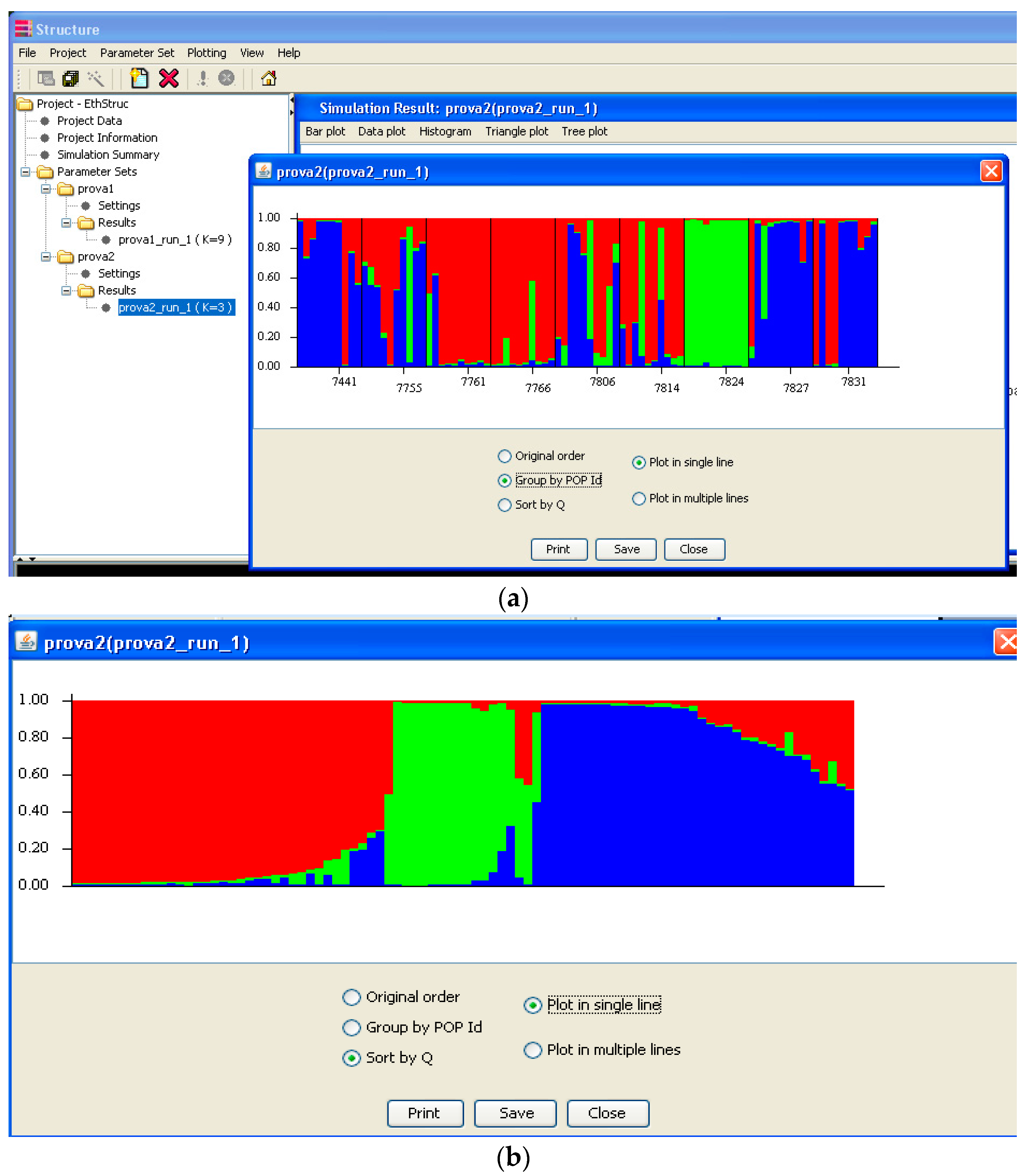
The Structure output can be displayed as a “triangle plot” in which two clusters are plotted at two vertices and all the others at the third (Figure 8). When more than three clusters are obtained, it can require further classification. However, a more useful, frequently used output is the bar plot on which the clusters are shown using different colors that can then be divided to highlight populations, or can be sorted by the Q value (Figure 9a,b). The picture gives a clear idea of how the individuals are divided among clusters/populations, and hence, the population similarity and the collections structure. Structure can provide the histograms of Fst, alpha, and likelihood for each cluster, as well as a tree plot of the distance among clusters. It is also possible to plot the average proportion of the Q values directly on a geographic map [30].

4. Conclusions

The different software packages available often use different methods and tools to describe populations.

Table 11. Comparison of different characteristics of most frequently used software.

Software	GenAlEx	GDA	Popgene	Power Marker	Cervus	Arlequin	Structure
Insert Data	Excel	Text	Text	Excel	Text	Text	Text
Descriptive Statistics
Genetic Diversity		X	X	X		X
Degree of Polymorphism	X		X	X
Heterozygosity	X	X	X	X	X	X
Expected Heterozygosity	X	X	X	X	X	X
Number of Alleles	X	X	X	X	X	X
Private Alleles		X
Effective Allele Number	X		X
PIC				X	X
Gene Flow			X
Homogeneity Test			X
Genetic Distance	X	X	X	X		X	X
Graphic Options		X	X	X			X
Fisher Parameters (Fis, Fit, Fst)	X	X	X			X
MANOVA	X					X
LD			X	X		X

provides an overview of the main function available for each program assessed in this paper. Overall, the author recommends using GenAlEx and/or Power Marker to insert data, subsequently exporting/importing and converting as required. In addition, either GDA and/or Power Marker can be used to perform most of the statistical analyses required for measuring genetic diversity, such as the percent of polymorphism, allele number, polymorphic allele number, and the expected and observed heterozygosity. In GDA, these parameters refer both to the loci and to the populations, while in Power Marker, several subsets of data should be run per population. Power Marker also computes PIC values, while GDA also computes private alleles. Both programs have different methodologies for computing population distance. Finally, GenAlEx and Arlequin are useful for determining analyses of molecular variance and Structure provides a clear illustration of population clustering.

References

- Mondini, L.; Noorani, A.; Pagnotta, M.A. Assessing Plant Genetic Diversity by Molecular Tools. Diversity 2009, 1, 19–35. [Google Scholar] [CrossRef] [Green Version]
- Hardy, G.H. Mendelian proportions in a mixed population. Science 1908, 28, 49–50. [Google Scholar] [CrossRef] [PubMed]
- Weinberg, W. On the demonstration of heredity in man. In Papers on Human Genetics (1963); Prentice Hall: Englewood Cliffs, NJ, USA, 1908. [Google Scholar]
- Nei, M. Analysis of Gene Diversity in Subdivided Populations. Proc. Natl. Acad. Sci. USA 1973, 70, 3321–3323. [Google Scholar] [CrossRef] [PubMed] [Green Version]
- Petit, R.J.; Mousadik, A.E.; Pons, O. Identifying Populations for Conservation on the Basis of Genetic Markers. Conserv. Biol. 1998, 12, 844–855. [Google Scholar] [CrossRef]
- Nei, M. Estimation of Average Heterozygosity and Genetic Distance from a Small Number of Individuals. Genetics 1978, 89, 583–590. [Google Scholar] [PubMed]
- Wright, S. The Interpretation of Population Structure by F-Statistics with Special Regard to Systems of Mating. Evolution 1965, 19, 395–420. [Google Scholar] [CrossRef]
- Turpeinen, T.; Tenhola, T.; Manninen, O.; Nevo, E.; Nissilä, E. Microsatellite diversity associated with ecological factors in Hordeum spontaneum populations in Israel. Mol. Ecol. 2001, 10, 1577–1591. [Google Scholar] [CrossRef]
- Botstein, D.; White, R.L.; Skolnick, M.; Davis, R.W. Construction of a genetic linkage map in man using restriction fragment length polymorphisms. Am. J. Hum. Genet. 1980, 32, 314–331. [Google Scholar]
- Nei, M. Genetic Distance between Populations. Am. Nat. 1972, 106, 283–292. [Google Scholar] [CrossRef]
- Nei, M.; Roychoudhury, A.K. Sampling Variances of Heterozygosity and Genetic Distance. Genetics 1974, 76, 379–390. [Google Scholar]
- Nei, M. Molecular Evolutionary Genetics; Columbia University Press: New York, NY, USA, 1987; 512p. [Google Scholar]
- Peakall, R.; Smouse, P.E. GenALEx 6: Genetic analysis in Excel. Population genetic software for teaching and research. Mol. Ecol. Notes 2006, 6, 288–295. [Google Scholar] [CrossRef]
- Lewis, P.O.; Zaykin, D. Genetic Data Analysis: Computer Program for the Analysis of Allelic Data, Version 1.0 (d16c), 2001. Free Program Distributed by the Authors over the Internet. 2012. Available online: http://lewis.eeb.uconn.edu/lewishome/software.html (accessed on 1 October 2018); https://phylogeny.uconn.edu/software/ (accessed on 5 December 2018).
- Yeh, F.C.; Yang, R.C.; Boyle, T.; Ye, Z.H.; Mao, J.X. POPGENE, Version 1.32: The User Friendly Software for Population Genetic Analysis; Molecular Biology and Biotechnology Centre, University of Alberta: Edmonton, AB, Canada, 1999. [Google Scholar]
- Liu, K.; Muse, S.V. PowerMarker: An integrated analysis environment for genetic marker analysis. Bioinformatics 2005, 21, 2128–2129. [Google Scholar] [CrossRef] [PubMed]
- Kalinowski, S.T.; Taper, M.L.; Marshall, T.C. Revising how the computer program cervus accommodates genotyping error increases success in paternity assignment. Mol. Ecol. 2007, 16, 1099–1106. [Google Scholar] [CrossRef] [PubMed]
- Excoffier, L.; Laval, G.; Schneider, S. Arlequin (version 3.0): An integrated software package for population genetics data analysis. Evol. Bioinform. Online 2005, 1. [Google Scholar] [CrossRef]
- Pritchard, J.K.; Stephens, M.; Donnelly, P. Inference of Population Structure Using Multilocus Genotype Data. Genetics 2000, 155, 945–959. [Google Scholar] [PubMed]
- Mondini, L.; Farina, A.; Porceddu, E.; Pagnotta, M.A. Analysis of durum wheat germplasm adapted to different climatic conditions. Ann. Appl. Biol. 2010, 156, 211–219. [Google Scholar] [CrossRef]
- Peakall, R.; Smouse, P.E. GenAlEx 6.5: Genetic analysis in Excel. Population genetic software for teaching and research—An update. Bioinformatics 2012, 28, 2537–2539. [Google Scholar] [CrossRef]
- Page, R.D. TreeView; Glasgow University: Glasgow, UK, 2001. [Google Scholar]
- Weir, B.S. Genetic data analysis. Methods for discrete population genetic data. In Genetic Data Analysis. Methods for Discrete Population Genetic Data; Sinauer Associates: Sunderland, MA, USA, 1990. [Google Scholar]
- Page, R.D.M. TREEVIEW: An Application to Display Phylogenetic Trees on Personal Computers. Comput. Appl. Biosci. Macintosh 1996, 12, 357–358. [Google Scholar]
- Excoffier, L.; Smouse, P.E.; Quattro, J.M. Analysis of Molecular Variance Inferred from Metric Distances among DNA Haplotypes: Application to Human Mitochondrial DNA Restriction Data. Genetics 1992, 131, 479–491. [Google Scholar]
- Lewontin, R.C.; Kojima, K. The Evolutionary Dynamics of Complex Polymorphisms. Evolution 1960, 14, 458–472. [Google Scholar] [CrossRef]
- Dixon, W.J.; Brown, M.B.; Engelman, L.; Jennrich, R.I. Multiple comparison tests. In BMDP Statistical Software Manual; University of California Press: Berkeley, CA, USA, 1990; pp. 196–200. [Google Scholar]
- Evanno, G.; Regnaut, S.; Goudet, J. Detecting the number of clusters of individuals using the software structure: A simulation study. Mol. Ecol. 2005, 14, 2611–2620. [Google Scholar] [CrossRef] [PubMed]
- Earl, D.A.; vonHoldt, B.M. STRUCTURE HARVESTER: A website and program for visualizing STRUCTURE output and implementing the Evanno method. Conserv. Genet. Resour. 2012, 4, 359–361. [Google Scholar] [CrossRef]
- Pagnotta, M.A.; Fernández, J.A.; Sonnante, G.; Egea-Gilabert, C. Genetic diversity and accession structure in European Cynara cardunculus collections. PLoS ONE 2017, 12, e0178770. [Google Scholar] [CrossRef] [PubMed]
Figure 1.
Diagram of the relationships between the gene diversity components. I = individual, S = subpopulation, T = total population.
Figure 2.
Structure of the data inserted by GenAlEx, the Excel macro for genetic analyses. (a) Template; (b) data in D sheet.
Figure 3.
Co-dominant frequency options of GenAlEx Excel macro.
Figure 4.
UPGMA dendrogram based on Nei genetic distance.
Figure 5.
Popgene input file and analyses options.
Figure 6.
Power Marker output for the genetic data.
Figure 7.
Power Marker output for the pairwise linkage disequilibrium.
Figure 8.
Structure output of the triangle plot with the relationships among clusters.
Figure 9.
Structure output of the bar plot clusters either by populations (a) or sorted by the Q value (b) are reported with different colors.