The Impact of Misspecified Random Effect Distribution in a Weibull Regression Mixed Model


1
Escuela de Estadística, Universidad Nacional de Colombia sede Medellín, Medellín 050034, Colombia
2
Instituto de Matemática e Estatística, Universidade de São Paulo, São Paulo 05508-090, Brazil
*
Author to whom correspondence should be addressed.
Stats 2018, 1(1), 48-76; https://doi.org/10.3390/stats1010005
Submission received: 17 March 2018
/
Revised: 25 May 2018
/
Accepted: 29 May 2018
/
Published: 31 May 2018
Abstract
:Mixed models are useful tools for analyzing clustered and longitudinal data. These models assume that random effects are normally distributed. However, this may be unrealistic or restrictive when representing information of the data. Several papers have been published to quantify the impacts of misspecification of the shape of the random effects in mixed models. Notably, these studies primarily concentrated their efforts on models with response variables that have normal, logistic and Poisson distributions, and the results were not conclusive. As such, we investigated the misspecification of the shape of the random effects in a Weibull regression mixed model with random intercepts in the two parameters of the Weibull distribution. Through an extensive simulation study considering six random effect distributions and assuming normality for the random effects in the estimation procedure, we found an impact of misspecification on the estimations of the fixed effects associated with the second parameter of the Weibull distribution. Additionally, the variance components of the model were also affected by the misspecification.
1. Introduction
Mixed models are useful tools for analyzing correlated, clustered and longitudinal data that arise from medical, social and behavioral sciences studies. However, this class of models makes a strong assumption about the distribution of random effects. For computational convenience, random effects are assumed to be normal, but this assumption may be unrealistic for some applications [1]. Since the random effects are not observable, checking the assumption is difficult, and if the true distribution of the random effects is far from normality, the estimation and inferences could be considerably affected.
In the literature, many studies have evaluated the impacts of mixed models that assume a normal distribution for random effects on several aspects related to the estimation and inference, when in fact the underlying distribution of the random effects is non-normal. This situation was called the “misspecification problem” by Neuhaus and McCulloch [2]. In these studies, the covariates are classified into two types. A covariate can be a “between-cluster” covariate, meaning that it is constant over the units in a cluster. Conversely, it can be a “within-cluster” covariate, which means that it varies within a cluster, but it has an average that is constant between clusters [3]. Some of these studies are summarized below.
Considering linear mixed models (LMM), Verbeke and Lesaffre [4] used simulations to show that maximum likelihood estimators for fixed effects and variance components are consistent and asymptotically normally distributed, even when the random effect distribution is not normal. Using the relative distance, the authors showed the clear consistency of the maximum likelihood estimators as the total sample size increased. Unfortunately, these conclusive results were not found for other classes of mixed models.
Neuhaus et al. [5] conducted a simulation of a logistic random model (LRM) in which gamma, t-Student and normal distributions were considered for the random effects. They estimated the model parameters assuming a normal distribution for the random effects and found that the estimated parameters were asymptotically biased, but the magnitude of the bias was typically small.
Heagerty and Kurland [6] considered an LRM in which the random effect followed one of four situations: a random intercept that was non-normally distributed, the variance of the random intercept, which depended on a between-cluster covariate, assuming a random intercept, when in fact there was a random intercept and slope, and autocorrelated random intercepts. Through a simulation study using relative bias, the authors found that incorrect assumptions regarding the random effects could lead to substantial bias in the estimates for the fixed effects when the random effect distribution depended on the measured covariates or when there was an autoregressive random effect.
Agresti et al. [7] showed that a considerable loss of efficiency occurred when the random effect distribution differs from the true distribution for three different models: LRM, random effects model for log odds ratio and frailty model.
Litière et al. [8] used simulations to study the impacts of the misspecification of the random effect distribution on the power of the Wald test for the fixed effect parameters in an LRM. Four true distributions for the random effects (normal, power function, discrete and a mixture of two normal) and each simulated dataset were fitted assuming normality for the random effects. They claimed that the misspecification of the random effect distribution could produce a marked increase or decrease in the power of the Wald test, depending on the shape of the random effect distribution.
Litière et al. [9] also studied the impact of misspecification on parameter estimation and hypothesis testing through simulations using an LRM based on a schizophrenia study considering nine different distributions of the random effects. These authors found that the estimates of the variance components were severely affected by the misspecification. Additionally, they found that the coefficient of the within-cluster covariate appeared to be less affected by the misspecification of the variance of less than four for the random effects. With respect to hypothesis testing, they found that misspecification severely affected the power of the test.
McCulloch and Neuhaus [3] used a simulation study to assess the impacts of misspecification on the inference of covariate effects, to estimate the random effects variance and to predict the random effects in an LRM. The authors used the Tukey distribution as the true distribution for random effects, and they fitted models assuming normal and Tukey (with known and unknown parameters) distributions for random effects. They found that the estimation of the intercept may be biased for a random effect distribution far from normal, and for the other parameters, the estimations had low biases. With respect to the prediction of random effects, they found that the mean square error of the prediction was slightly higher for the assumed normal distribution.
Neuhaus et al. [10] were not in agreement with Litière et al. [8] with respect to the LRM. They reanalyzed the scenarios and found that the misspecification of the shape of the random effect distribution led to a minimal increase in the Type II error. Moreover, to demonstrate the effects of misspecification, they argued that the assumed distribution needs to vary while the true distribution is held constant.
Litière et al. [11] presented a rejoinder to Neuhaus et al. [10], in which they defended the approach of varying the true underlying distribution for the random effects while fitting the model by assuming a normal distribution. Litière et al. considered an LRM and argued that, by using both approaches, the power associated with the test for the fixed-effect parameters in the logistic random model may be affected by misspecifying the random-effect distribution.
McCulloch and Neuhaus [12] used theory and a simulation study to investigate the impacts of the misspecification of the random effect distribution on how well the predicted values recover the true underlying distribution and the accuracy of the prediction of the realized values of the random effects. They considered two situations: LMM and LRM, with three random effect distributions. For each generated dataset, the model was fitted by assuming normal and exponential distributions for the random effects. The authors found that the shape of the distribution of the predictions of the random effects did not necessarily match the shape of the true distribution. In addition, the use of an incorrect distribution for the random effects only caused modest degradation of the mean square error of the prediction.
Neuhaus et al. [13] analyzed the impacts of the misspecification on the shape of the joint distribution of the random intercepts and slopes on the estimates and confidence intervals for generalized linear mixed models (GLMM). Through analytical and simulation studies, the estimates of the covariate effects showed little bias.
As shown, until now, most simulation studies focused on LRM or GLMM, and no significant studies have considered other classes of mixed models or other distributions for the response variable. The Weibull distribution is one of the most popular distributions associated with the models that can be applied to diverse areas ranging from engineering (reliability), health (survival analysis) and ecology (Fleming [14], Carroll [15], Abdel-Ghaly et al. [16]). The contribution of this paper is to explore the impacts of a misspecified random effect distribution on the estimation of the parameters in a mixed model with a response variable that follows a Weibull distribution.
Our paper is organized as follows. In Section 2, we present a case study of the lifetime of rubber in an abrasive process. In Section 3, we define the mixed model under consideration. In Section 4, we present the structures and the scenarios that were used in the simulation study, and in Section 5, we analyze the results of the simulation. The final Section 6 provides some concluding remarks.
2. A Case Study of Lifetime in an Abrasive Process
The data were obtained from an experimental design to study the effect of the density, torque, viscosity and temperature on the wear time of rubber pieces in an abrasive process. Ten pieces were analyzed, and each piece was cut into 15 small sub-pieces. For each piece, the density (g/cm) and the viscosity (Mooney viscosity) were measured; in the abrasive experiment, for each sup-piece, the torque (Tan ) and temperature (°C) were measured. The test involved submitting each sub-piece to an abrasive process to measure the wear time (minutes). Figure 1 depicts the empirical density (left) over time and boxplots for the time for the piece (right). The mean time was 12.9 min with a standard deviation of 8.9 min.
In this application, we have clustered data because several sub-pieces were obtained from a specific piece. In this situation, it was appropriate to consider a mixed model to model the response variable. The variables density and viscosity were between-cluster covariates because they were measured over pieces; whereas torque and temperature were measured over the sub-pieces. Several mixed models were fitted to explain the of the sub-piece j within piece i where and . Using the Akaike information criterion () proposed by Akaike [17] and the Schwarz Bayesian criterion () proposed by Schwarz [18], the best mixed model for the dataset had a response variable showing a Weibull distribution, and the model can be summarized as:
3. Weibull Regression Mixed Model
The Weibull distribution was named after Swedish mathematician Waloddi Weibull (1887–1979). This distribution is important because it describes the failure times of many different phenomena [19]. The Weibull distribution has been extensively used and cited in the fields of engineering, chemistry, meteorology, material science, medicine, quality control and biology. More details about the applications were provided by Murthy et al. [20] and Rinne [21].
The importance of the Weibull distribution can be viewed in terms of the parameterizations that were proposed in the literature. Almalki and Nadarajah [22] provided an extensive review of 29 modifications of the Weibull distribution. Bagheri et al. [23] proposed the generalized modified Weibull power series distribution that contains, as special cases, several important distributions that are modifications of the Weibull distribution. Domma et al. [24] proposed the generalized weighted Weibull distribution that includes decreasing, increasing, upside-down bathtub, N-shape and M-shape hazard rates.
In the literature, some regression models have used the Weibull distribution. Silva et al. [25] proposed a log-extended Weibull regression model to analyze survival time for patients with cancer using the performance status at diagnosis, a measure of general fitness, the age of the patient and the number of months since the cancer diagnosis as explanatory variables. Vigas et al. [26] used the Poisson–Weibull distribution to explain the survival time of the patients who were admitted into a heart transplant program using the year of acceptance to the program, the age of the patient, information about previous surgery (where one was yes and zero was no) and if the patient had the transplant within the program (where one was yes and zero was no) as covariates. Prataviera et al. [27] considered a generalized odd log-logistic flexible Weibull regression model to explain the breaking time for a part located in a sugarcane cutting system using the agent causing the failure as the covariate.
Mixed Weibull models have been also used to analyze real datasets. Sohn et al. [28] used a random effects Weibull model to explain the reliability of modules in a fighter aircraft based on the characteristics and operational conditions of the plane. Sohn et al. [29] considered a random effects Weibull regression model to study the occupational lifetime of the employees who join another company, based on characteristics such as position, gender, marriage status and age, among others. Bartolucci et al. [30] proposed a Bayesian mixed Weibull model to explore the survival time of patients with myelodysplastic syndrome by comparing the efficacy and toxicity of two treatments. Lv et al. [31] used a mixed Weibull model for data from a design experiment to explain the lifetime of a thermostat using 12 low- or high-level explanatory variables.
The original Weibull distribution has several parameterizations; however, in this work, we used the parameterization called , which can be found in Stasinopoulos and Rigby [32]. The probability density function, mean and variance for the parameterization are as follows:
where and is the gamma function.
Assuming that is the j-th observation for the i-th cluster and conditional on the independent random intercepts and , the response variable is distributed as an independent random variable with a Weibull distribution as follows:
where represents the number of clusters and represents the number of observations within cluster i. In the model (5), and are known design matrices for the cluster i; thus, and correspond to the j-th rows of and respectively, and and are vectors of unknown fixed effects. The log function included in the model (5) ensures that the linear predictors for and map to the appropriate values for and , respectively. The model assumes that and and uncorrelated. Then, the parameter vector for the model (5) is .
The likelihood function for the i-th cluster is given by:
where is the probability density function of and corresponds to the normal density with zero mean and variance . The integrals in Equation (6) do not have a closed form, and approximations are required for a computationally-feasible estimation [33]. In this work, we used the Gauss–Hermite quadrature (GHQ) approximation to obtain Equation (6). We choose the maximum likelihood method to obtain the estimates for the parameter vector , in which the objective is to maximize the log-likelihood function given by:
4. Simulation Study
We performed a simulation study to evaluate the impacts of misspecification on the estimation of parameters. We adopted the approach used by Verbeke and Lesaffre [4], Agresti et al. [7], Litière et al. [8], Litière et al. [9], Litière et al. [11], Alonso et al. [34] and Alonso et al. [35], in which we varied the true distribution of the random effects while the assumed distribution remained constant. For the random intercepts and , we considered six different distributions: normal, uniform, exponential, log-gamma, log-normal and symmetric mixture of two normal densities that were defined as in McCulloch and Neuhaus [12]. The distributions were transformed such that the zero-mean condition was satisfied, and the corresponding variances were equal to the prespecified values and for and , respectively. Figure 2 shows the respective densities for the case with unit variance. With this choice, we cover a range of densities varying from very symmetric to very skewed distributions.
For the simulation study, we considered the next model:
with being the number of clusters and the number of observations per cluster. The variables and represent between-cluster covariates, whereas and represent within-cluster covariates. We considered , , and distributed as . The vector parameter in the simulation study is given by .
The true values for the fixed parameters in the simulation were chosen to ensure that the datasets had a response variable with mean and variance of approximately 12 and nine, respectively. The fixed effects were considered constant with the following values: , , , , , . This selection emulated the dataset shown in Section 2.
We considered equal variances for the random intercepts and , and these variances were 0.5, 1.0, 1.5 and 2.0. The variances greater than 2.0 were not considered because they caused larger values of and , which directly affected the parameters and , which increased the variance that depends on and shown in Equation (4). We considered a variety of different numbers of clusters and observations per cluster, and the values were 5, 10, 15, 20, …, 45, 50 and 5, 10, 15, 20.
The simulation study included 960 cases, given by 6 distributions and 4 variances for the random intercepts, 10 values of N and 4 values of . For each distribution setting, the variance, N and , we generated 1000 samples with the model given by Equation (8). For each sample, we obtained the estimates of for the parameter vector that maximized the log-likelihood function in Equation (7) using our own code in R Core Team [36].
As in Verbeke and Lesaffre [4], we used the relative distance () to quantify the impact of the misspecification on the estimates. The relative distance is defined as
The smaller the value of the relative distance, the lower the impact. We also studied the impact of the misspecification on the estimation procedure using the median of .
5. Results
In this section, we present the results of the simulation study that was conducted to evaluate the impact of the misspecification of the random effect distribution in a Weibull mixed model as defined in Equation (8). The results are shown using figures that are provided in the Appendix A.
5.1. Relative Distance between the Estimated Parameter Vector and the True Parameter Vector
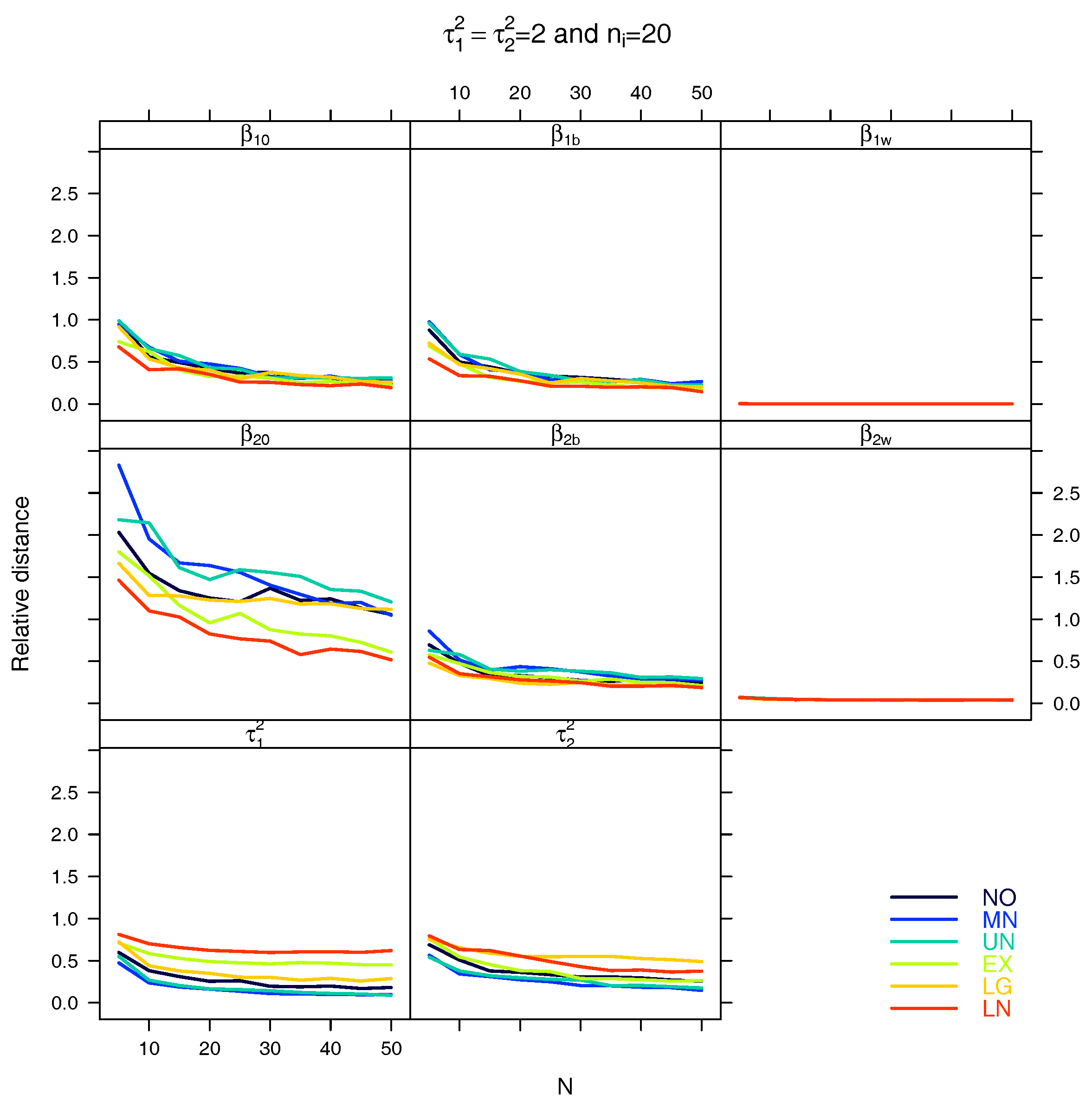
In Figure A1, Figure A2, Figure A3 and Figure A4, we can observe the median of the relative distance between the estimated parameter vector and the true parameter vector versus N for several combinations of and . Blue was assigned to the symmetric distributions (,,), whereas green, orange and red (,,) correspond to exponential, log-gamma and log-normal (asymmetric distributions), respectively. Dark blue (
) corresponds to the normal distribution used as the reference case. Figure A1, Figure A2, Figure A3 and Figure A4 have the same y-axis scale to facilitate comparison.
In each figure, the expected pattern of the relative distance decreasing as the number of clusters N increasing is observed. Additionally, we note an increase in the relative distance as the variances increase.
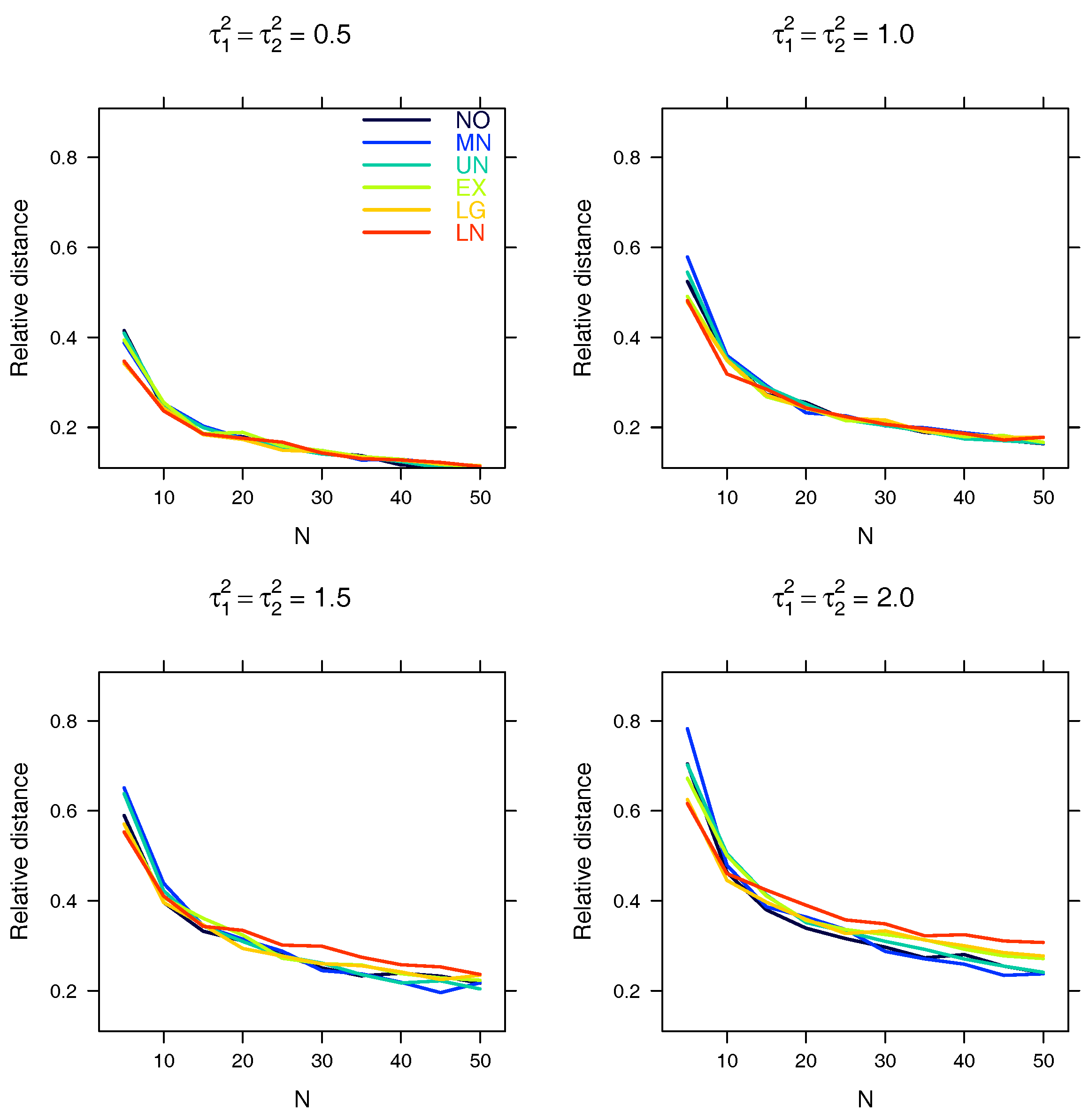
If we compare the corresponding panels in Figure A1, Figure A2, Figure A3 and Figure A4, the relative distance decreases as the number of observations per cluster increases, due to the increase in the number observations available to estimate the parameter vector .
From the third and fourth panels in Figure A2, Figure A3 and Figure A4, the blue lines tend to be below the asymmetric distributions (,,) when . This means that when asymmetric distributions are used to generate the random intercepts and the model is fitted assuming normality for the random intercepts, the estimated parameter vector is far from .
5.2. Relative Distance between the Estimated Parameter and the True Parameter
In Figure A5, Figure A6, Figure A7, Figure A8, Figure A9, Figure A10, Figure A11, Figure A12, Figure A13, Figure A14, Figure A15, Figure A16, Figure A17, Figure A18, Figure A19 and Figure A20, the medians are displayed of the relative distance between the estimated parameter and the true parameter versus N for several combinations of and . Again, blue was assigned to the symmetric distributions (
,,), whereas green, orange and red (,,) correspond to exponential, log-gamma and log-normal (asymmetric distributions), respectively. Dark blue () corresponds to the normal distribution used as the reference case. In these figures, six colored lines are found within each panel, excluding the panels for and in which the red line () intersects the other lines. The y-axis has different scales that clearly show the variability in the relative distance in each case.
By analyzing Figure A5, Figure A6, Figure A7, Figure A8, Figure A9, Figure A10, Figure A11, Figure A12, Figure A13, Figure A14, Figure A15, Figure A16, Figure A17, Figure A18, Figure A19 and Figure A20, we note that the relative distance for each estimated parameter decreases as N increases, except for and , in which the relative distance appears to be constant. The intercept shows the largest relative distance. By comparing Figure A5, Figure A6, Figure A7 and Figure A8, in which is constant at 0.5, the relative distance decreases as incrementally increases. This pattern is also observed in Figure A9, Figure A10, Figure A11, Figure A12, Figure A13, Figure A14, Figure A15, Figure A16, Figure A17, Figure A18, Figure A19 and Figure A20 when the variances are 1, 1.5 and 2. If the figures are compared with fixed, the relative distance increases as the variances increase.
The relative distance curves for the estimations of , , , and present the same shape as in Figure A5, Figure A6, Figure A7, Figure A8, Figure A9, Figure A10, Figure A11, Figure A12, Figure A13, Figure A14, Figure A15, Figure A16, Figure A17, Figure A18, Figure A19 and Figure A20 in which all colored lines tend to be near each other. In fact, for the estimated fixed coefficients ( and ) associated with the within variables, the relative distance curves are close. For this reason, we see only the red line that was drawn last.
For the estimated intercept , we note that the lines are slightly separated, but all lines show the same pattern. In half of the figures, the red line (log-normal) has a lower relative distance.
From Figure A5, Figure A6, Figure A7, Figure A8, Figure A9, Figure A10, Figure A11, Figure A12, Figure A13, Figure A14, Figure A15, Figure A16, Figure A17, Figure A18, Figure A19 and Figure A20, the blue lines (symmetric distributions) tend to be below the other lines (asymmetric distributions) as increases in the estimations for and . This means that when the random intercepts have asymmetric distributions, the estimated variances tend to have large relative distances.
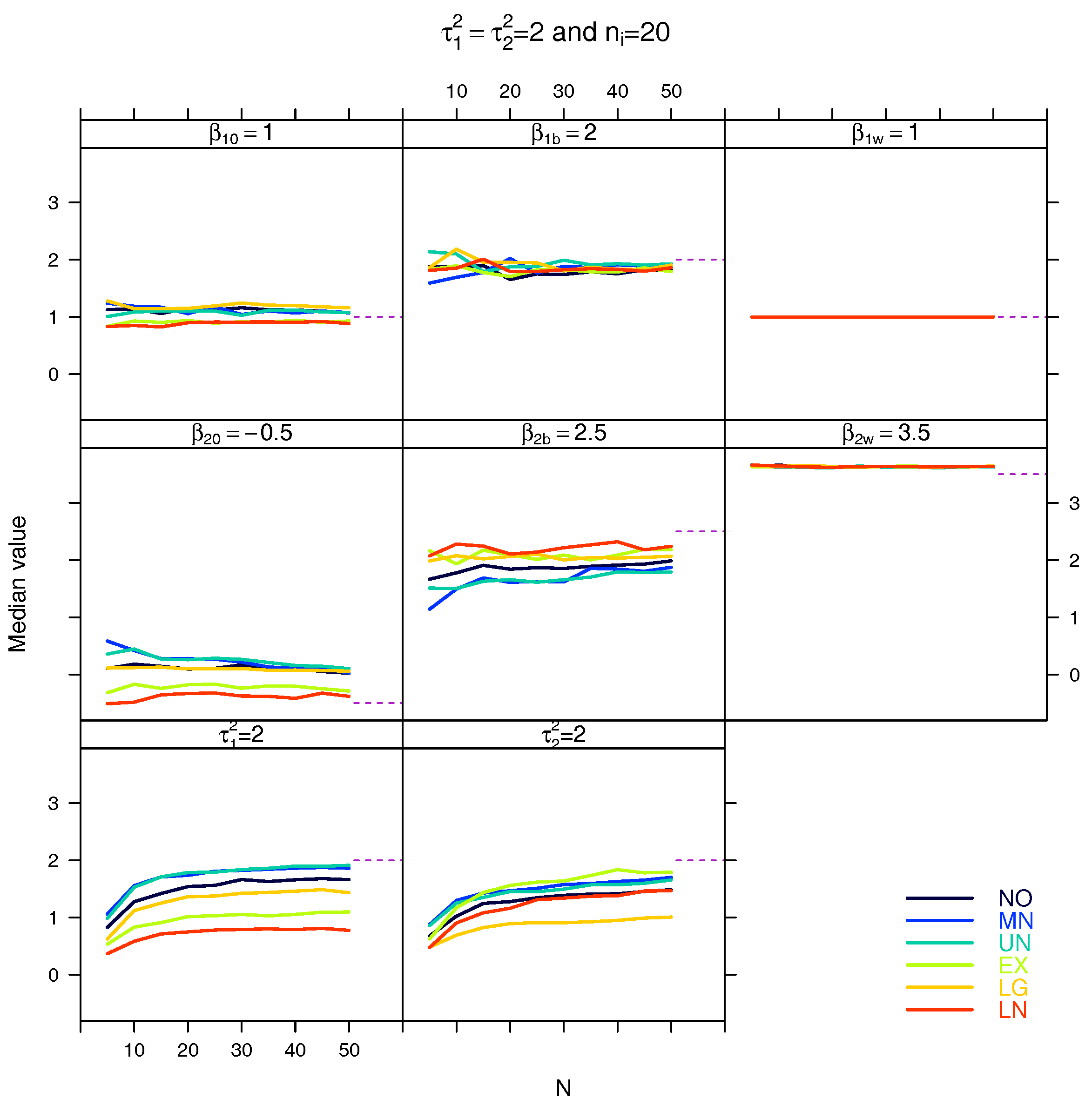
5.3. Median for the Estimated Fixed Parameters
Figure A21, Figure A22, Figure A23, Figure A24, Figure A25, Figure A26, Figure A27, Figure A28, Figure A29, Figure A30, Figure A31, Figure A32, Figure A33, Figure A34, Figure A35 and Figure A36 demonstrate the median for the estimated parameters obtained in the simulation study versus N for several combinations of and . Within each panel, the true value for the parameter and a dashed purple line () on the right side of the panel are included to identify if the estimators converge to the correct value.
Figure A21, Figure A22, Figure A23, Figure A24, Figure A25, Figure A26, Figure A27, Figure A28, Figure A29, Figure A30, Figure A31, Figure A32, Figure A33, Figure A34, Figure A35 and Figure A36 show some similar patterns. In all figures, the estimations for have a small bias that decreases as increases. As the variances of the random intercepts increase, the estimations for have a small bias when the true distributions of the random intercepts are normal, a mixture of normal, uniform and log-gamma. When the variances of the random effects are 1.5 or two, the estimations for tend to have a bias when the true distributions for the random intercepts are normal, a mixture of normal, uniform and log-gamma. The estimations for the variance components () tend to have a bias when the true distributions for the random intercepts are log-gamma and log-normal.
6. Conclusions
This simulation study was conducted to explore the impacts of a misspecified random effect distribution in a Weibull mixed model. The datasets for the study were simulated following six different distributions for random intercepts, but assuming normality for the random intercepts in the parameter estimation procedure. Two measures were used to evaluate the impacts of the misspecification on the parameter estimation, the relative distance and the median of the estimated parameters.
In Section 5.1, we calculated the relative distance between the estimated parameter vector and the true parameter vector . We found that when the true distributions of the random intercepts were exponential, log-gamma and log-normal (asymmetric distributions), the relative distance tended to be higher for , variances 1.5, 2.0 and . This means that when the true distributions for the random intercepts are asymmetric, the estimated vector tends to be far from the true vector .
In Section 5.2, the individual relative distance was obtained between each estimated parameter and the true parameter . The intercept demonstrated the largest relative distance, and the estimates of the variance components were severely affected when the random intercepts had an asymmetric distribution.
In Section 5.3, the median for each estimated parameter was obtained. From these results, we observed a large bias for that was not identified with the individual relative distance. However, the bias decreased as increased. We noted a bias in and for all distributions that were used to simulate the random intercepts. This bias tended to be higher for normal, mixture of normal, uniform and log-gamma when 1.5, 2. Additionally, we identified a remarkable bias in the estimated variance components when 1.5, 2 and the random intercepts had exponential, log-gamma, and log-normal distributions.
Despite that we did not consider the variances for random effects higher than two in the simulation study, we think that this could severely impact the measures for the cases when the random effects have asymmetric distributions (exponential, log-gamma and log-normal).
With these findings, we conclude that the misspecification impacts the estimations for the fixed effects and associated with the second parameter of the Weibull distribution. Additionally, the variance components and were also affected by the misspecification. For these reasons, in practice, we recommend checking the random effect distribution using diagnostic tests as proposed by Drikvandi et al. [37] and Efendi et al. [38]. Then, if the random effect distribution is not normal, use flexible procedures by considering non-normal distributions for the random effects to estimate the model parameters.
Overall, the misspecification of the random effects significantly impacts the estimation of all the parameters of the Weibull mixed model mainly when the distribution of the random effects is asymmetric.
Author Contributions
F.H. and V.G. wrote the paper and developed the simulation study together.
Acknowledgments
The authors would like to thank the research funding agencies CAPES and CNPq for the scholarships granted to the post-graduate student participating in the study.
Conflicts of Interest
The authors declare no conflict of interest.
Abbreviations
The following abbreviations are used in this manuscript:
| GLMM | Generalized linear mixed model |
| LMM | Linear mixed model |
| LRM | Logistic random model |
| Third parameterization of Weibull distribution | |
| GHQ | Gauss–Hermite quadrature |
| Relative distance |
Appendix A
Next are the figures for Section 5.1.
Figure A1.
Median of relative distance between and versus N for .
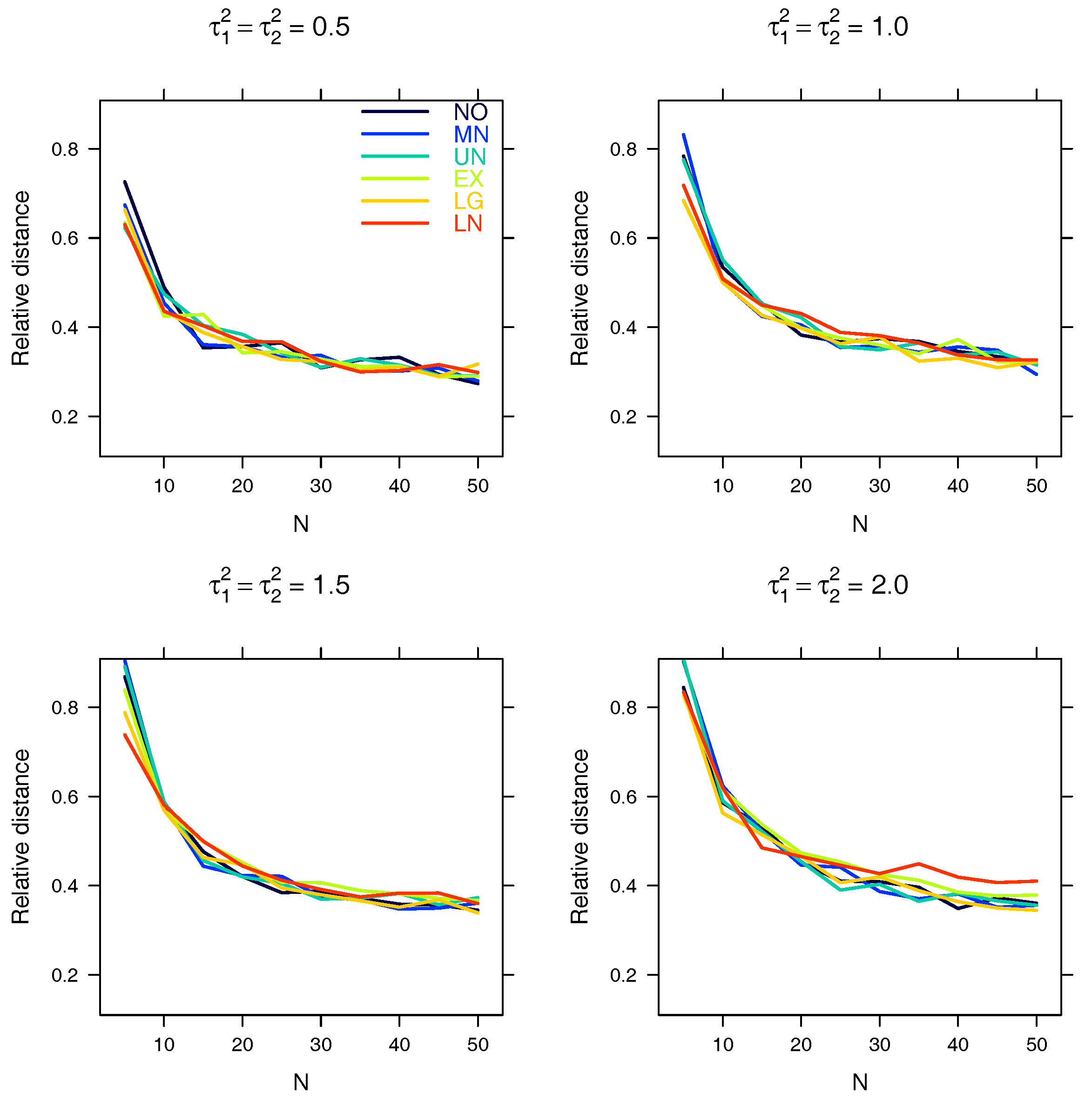
Figure A2.
Median of relative distance between and versus N for .
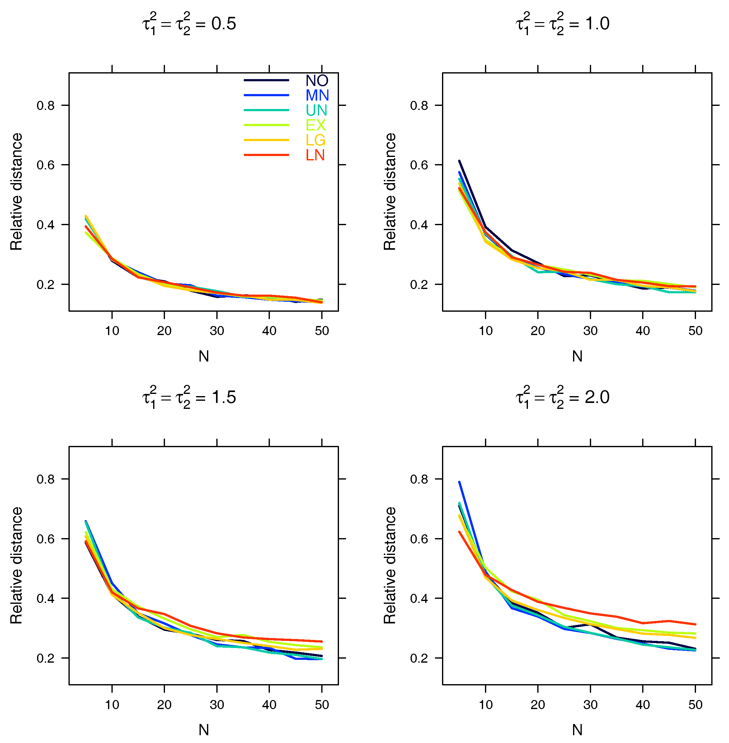
Figure A3.
Median of relative distance between and versus N for .
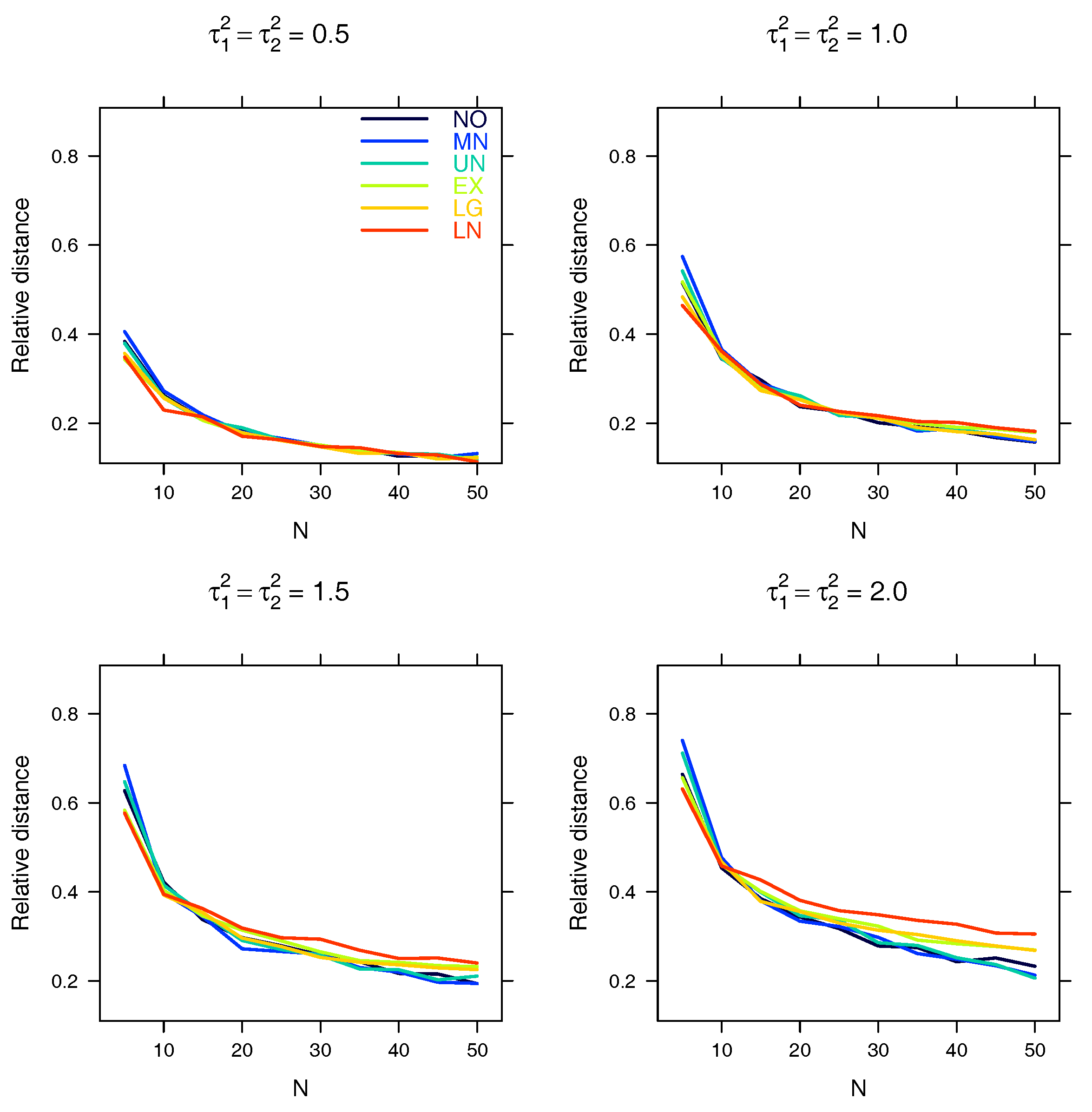
Figure A4.
Median of relative distance between and versus N for .
Next are the figures for Section 5.2.
Figure A5.
Median of relative distance between and versus N for with and .
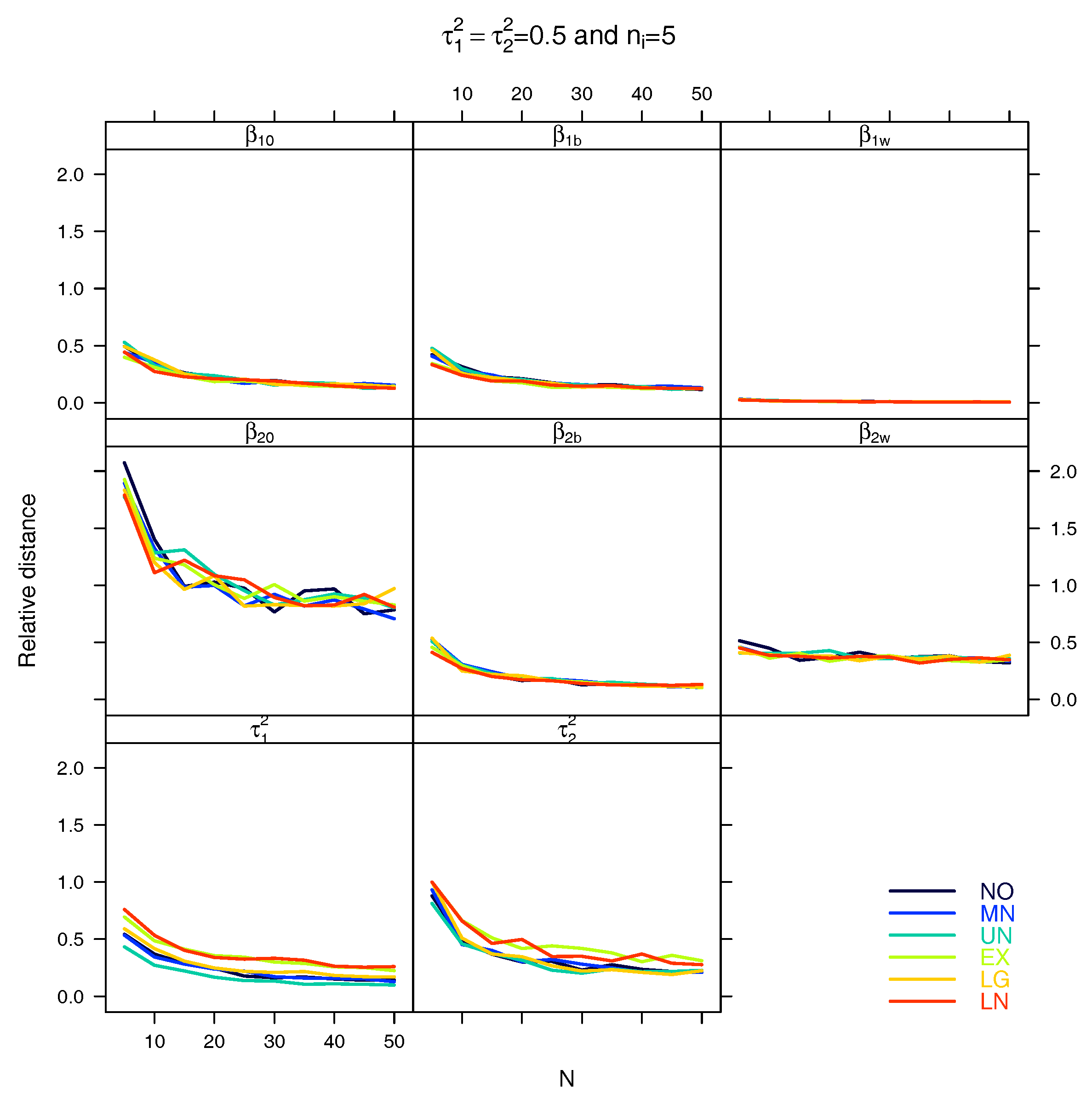
Figure A6.
Median of relative distance between and versus N for with and .
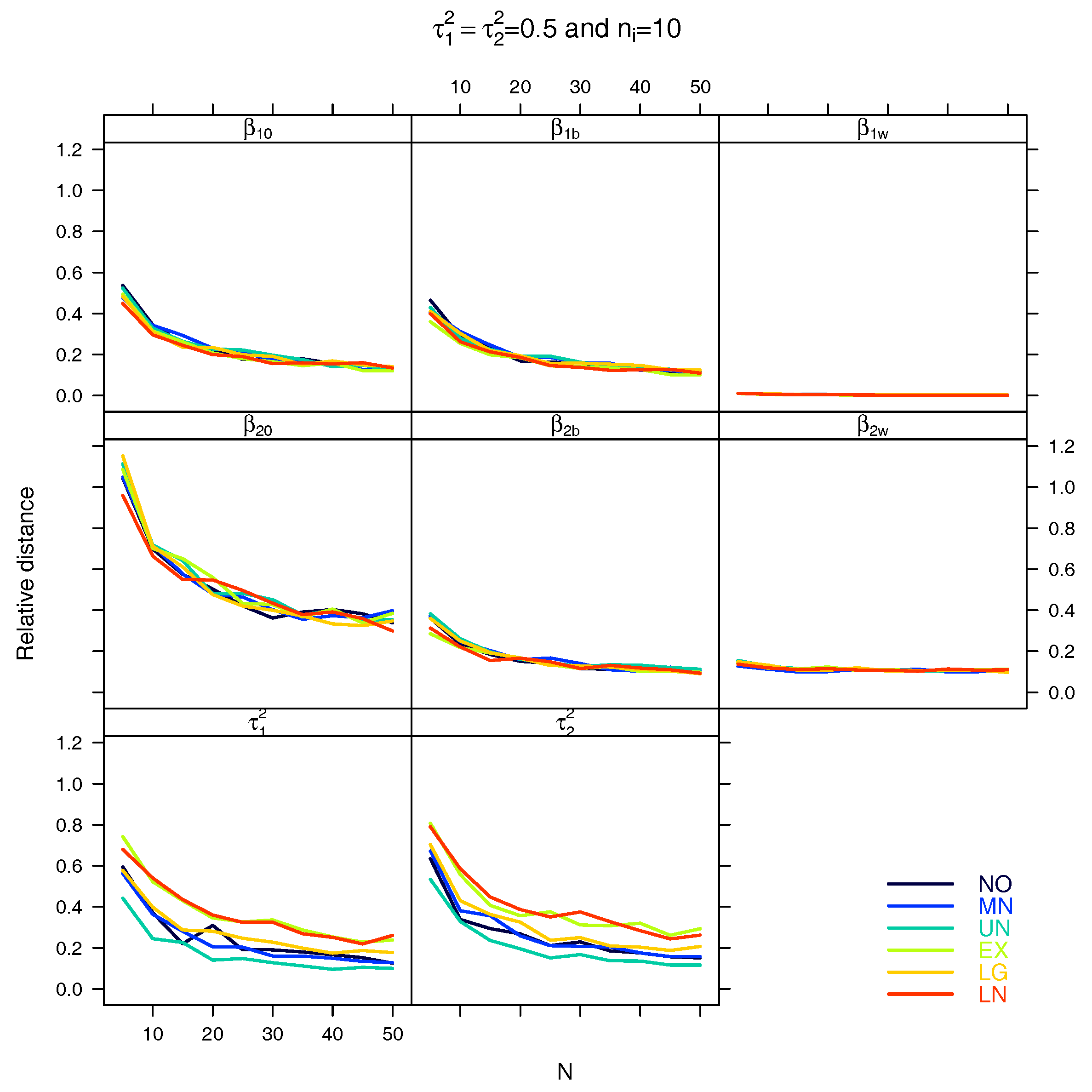
Figure A7.
Median of relative distance between and versus N for with and .

Figure A8.
Median of relative distance between and versus N for with and .
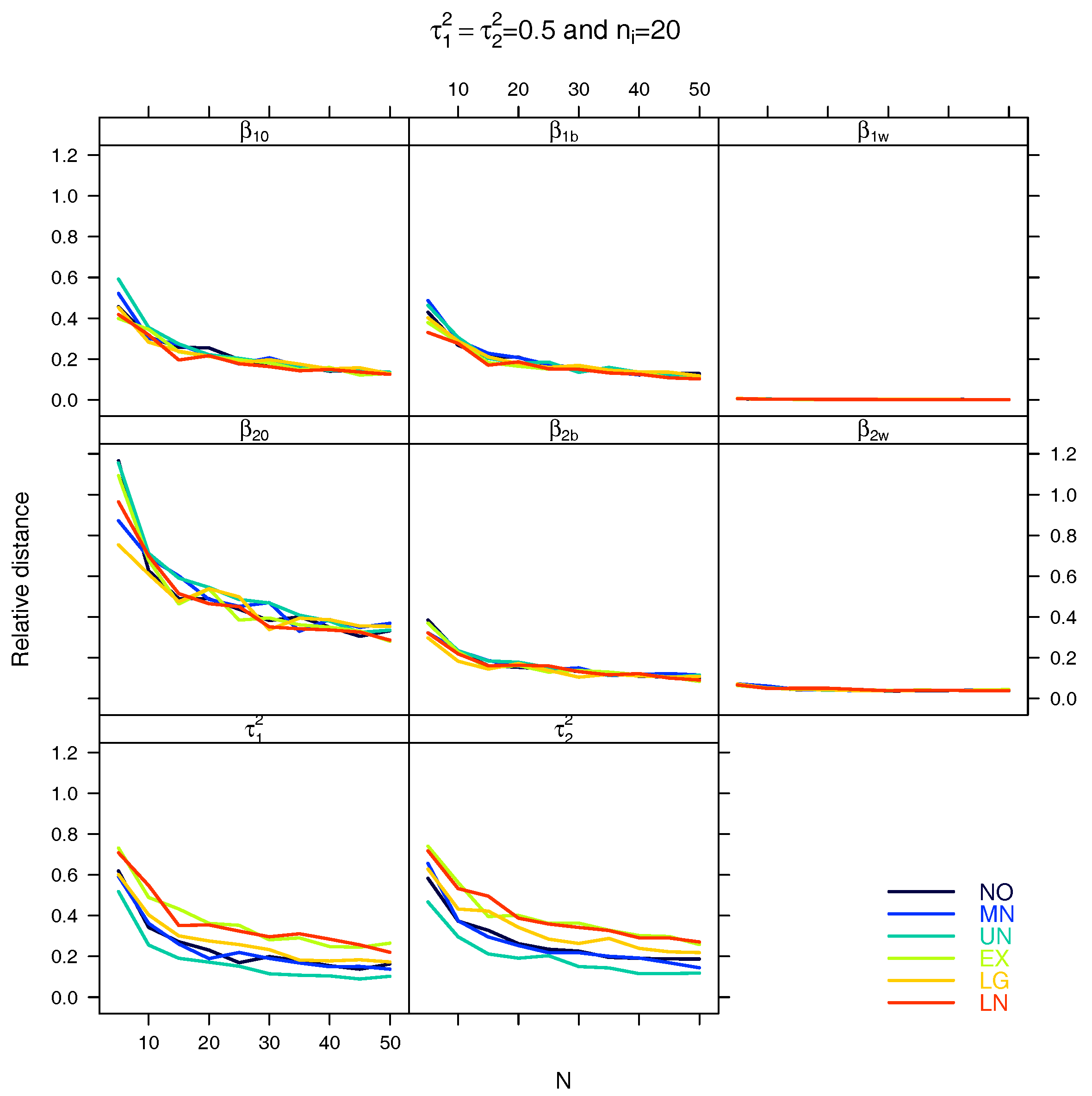
Figure A9.
Median of relative distance between and versus N for with and .
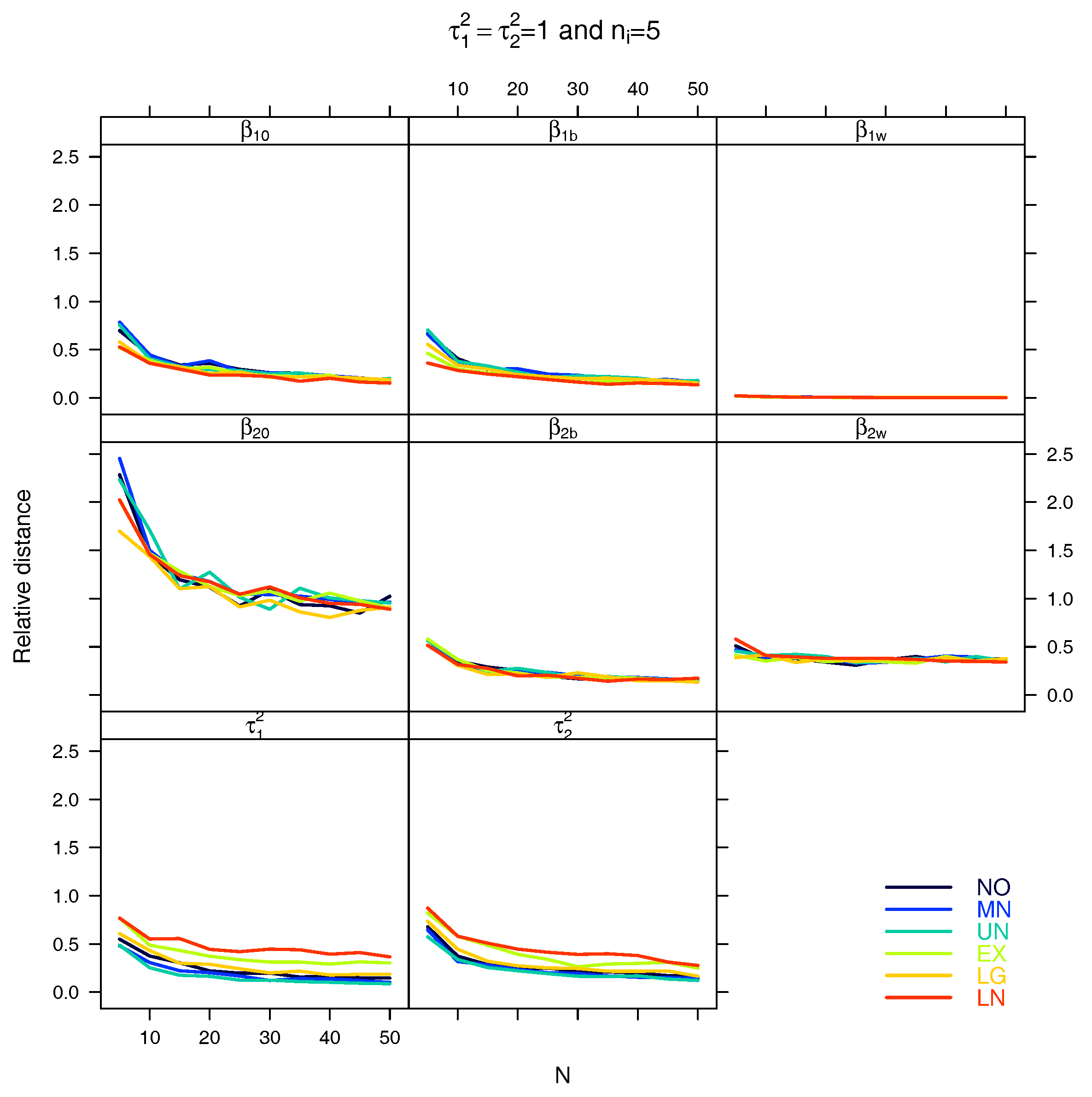
Figure A10.
Median of relative distance between and versus N for with and .
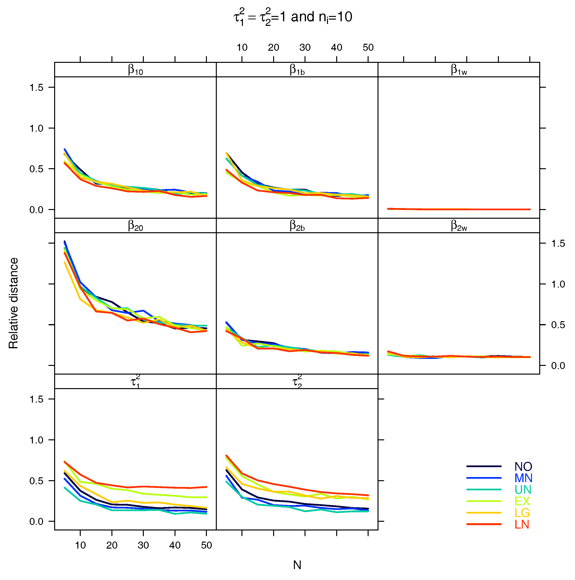
Figure A11.
Median of relative distance between and versus N for with and .

Figure A12.
Median of relative distance between and versus N for with and .
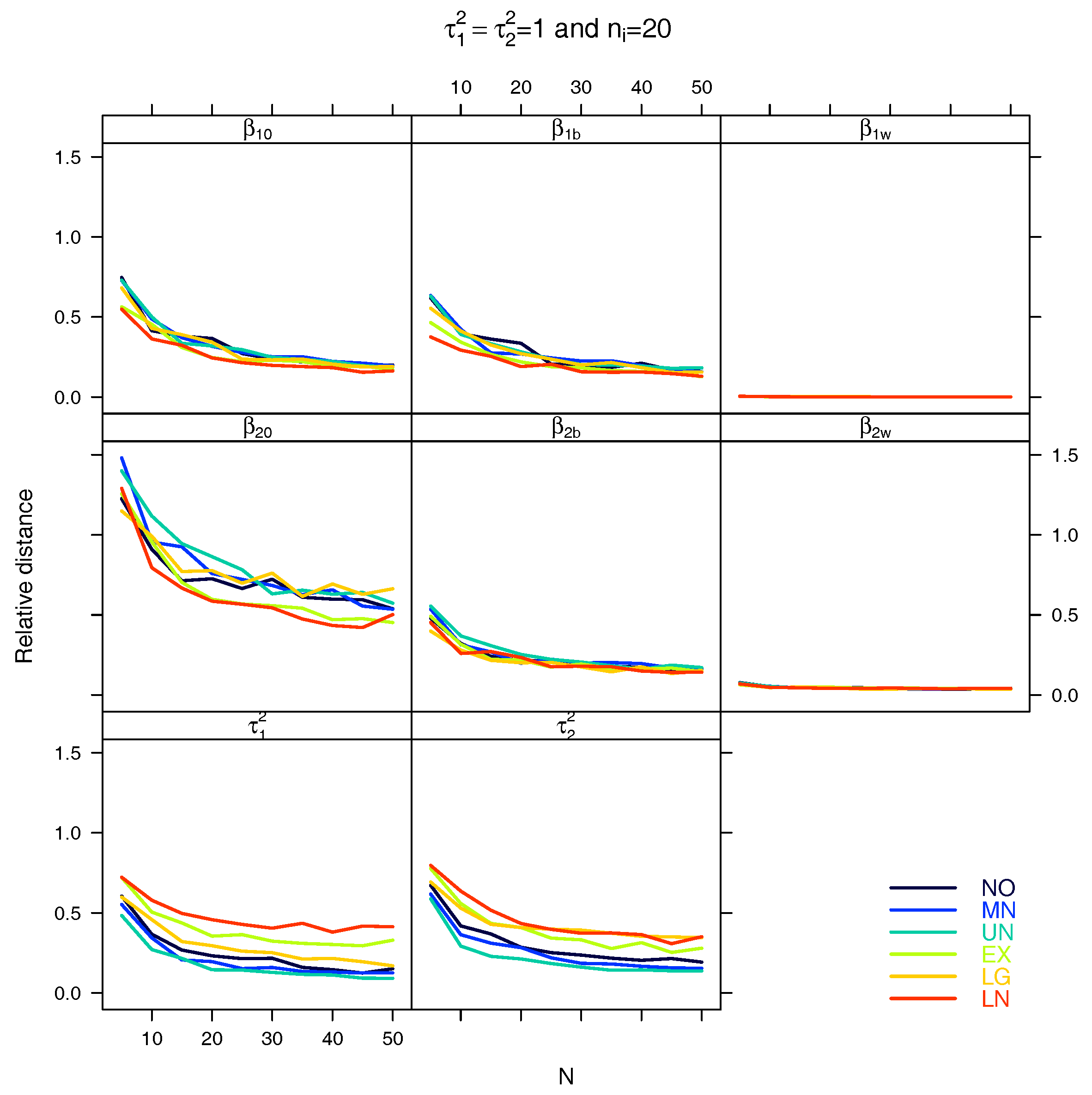
Figure A13.
Median of relative distance between and versus N for with and .
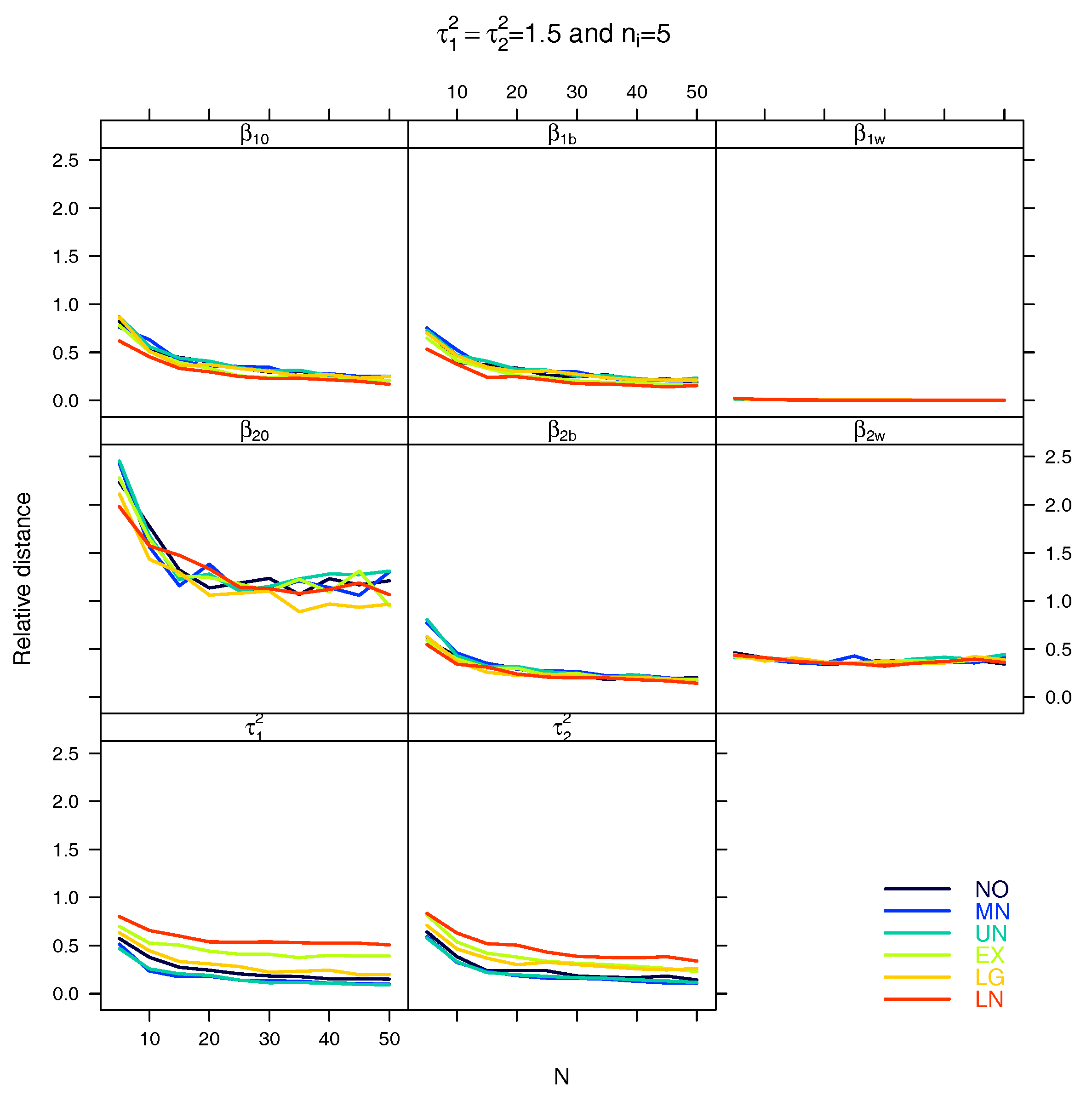
Figure A14.
Median of relative distance between and versus N for with and .
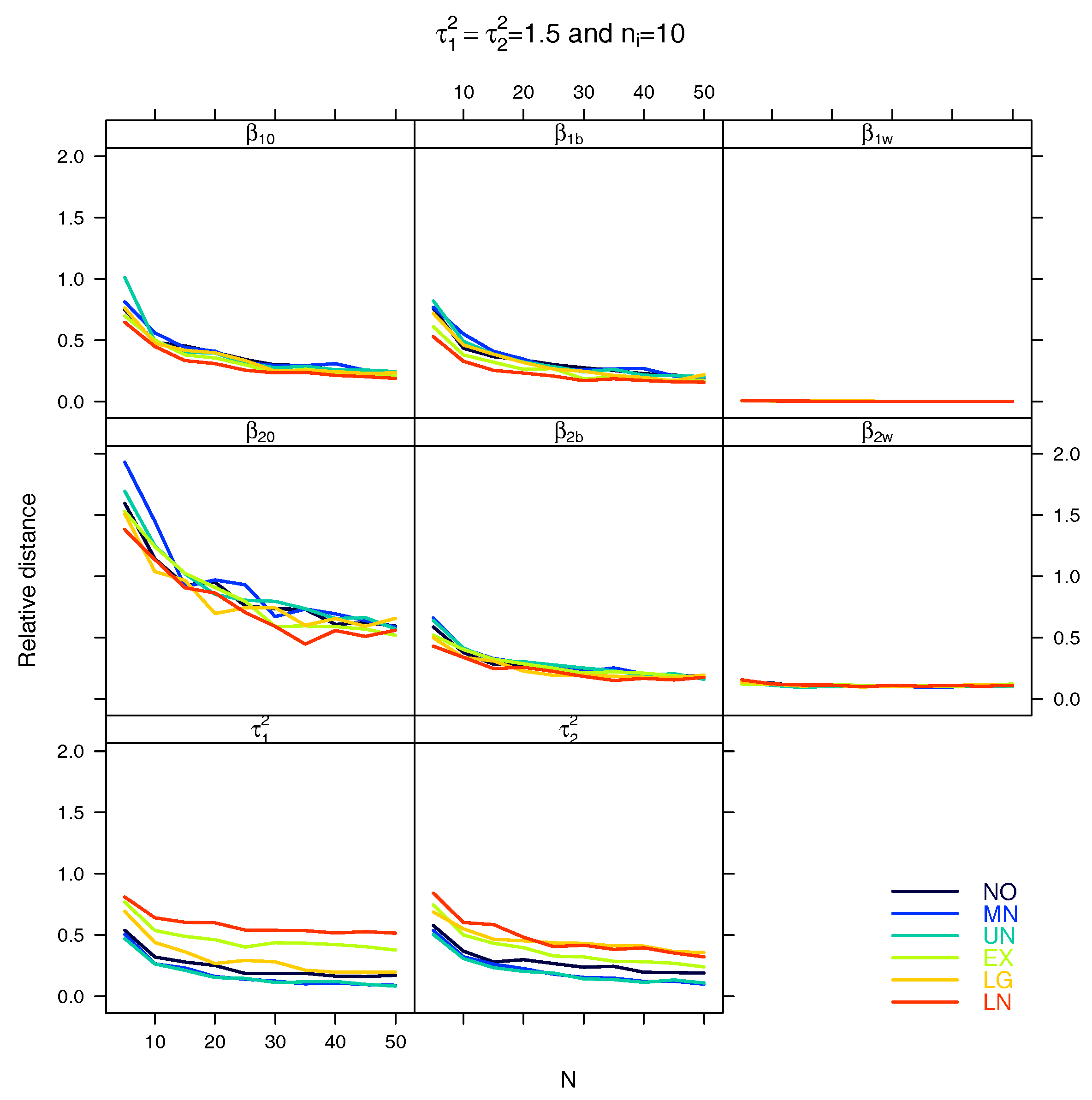
Figure A15.
Median of relative distance between and versus N for with and .
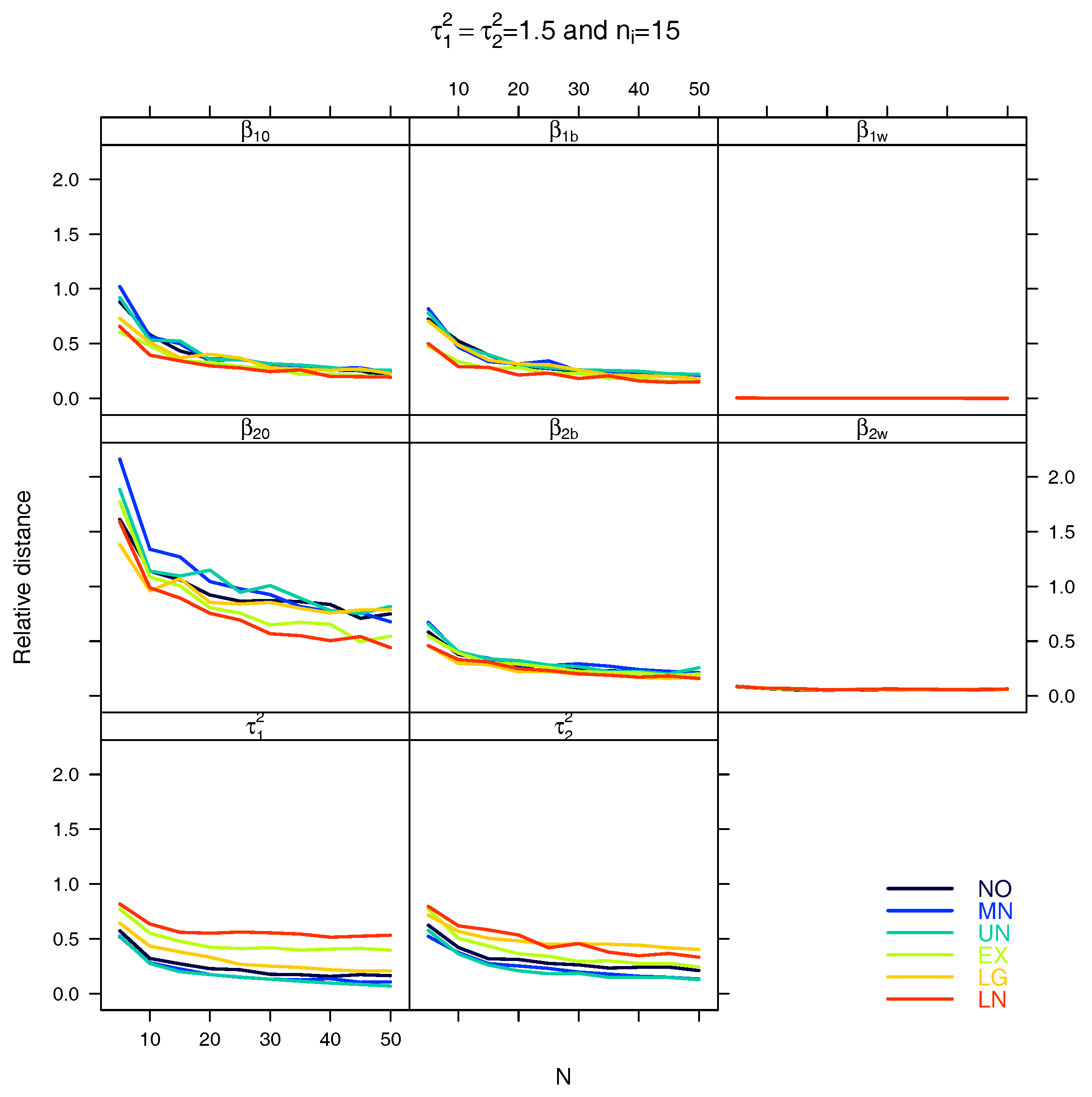
Figure A16.
Median of relative distance between and versus N for with and .
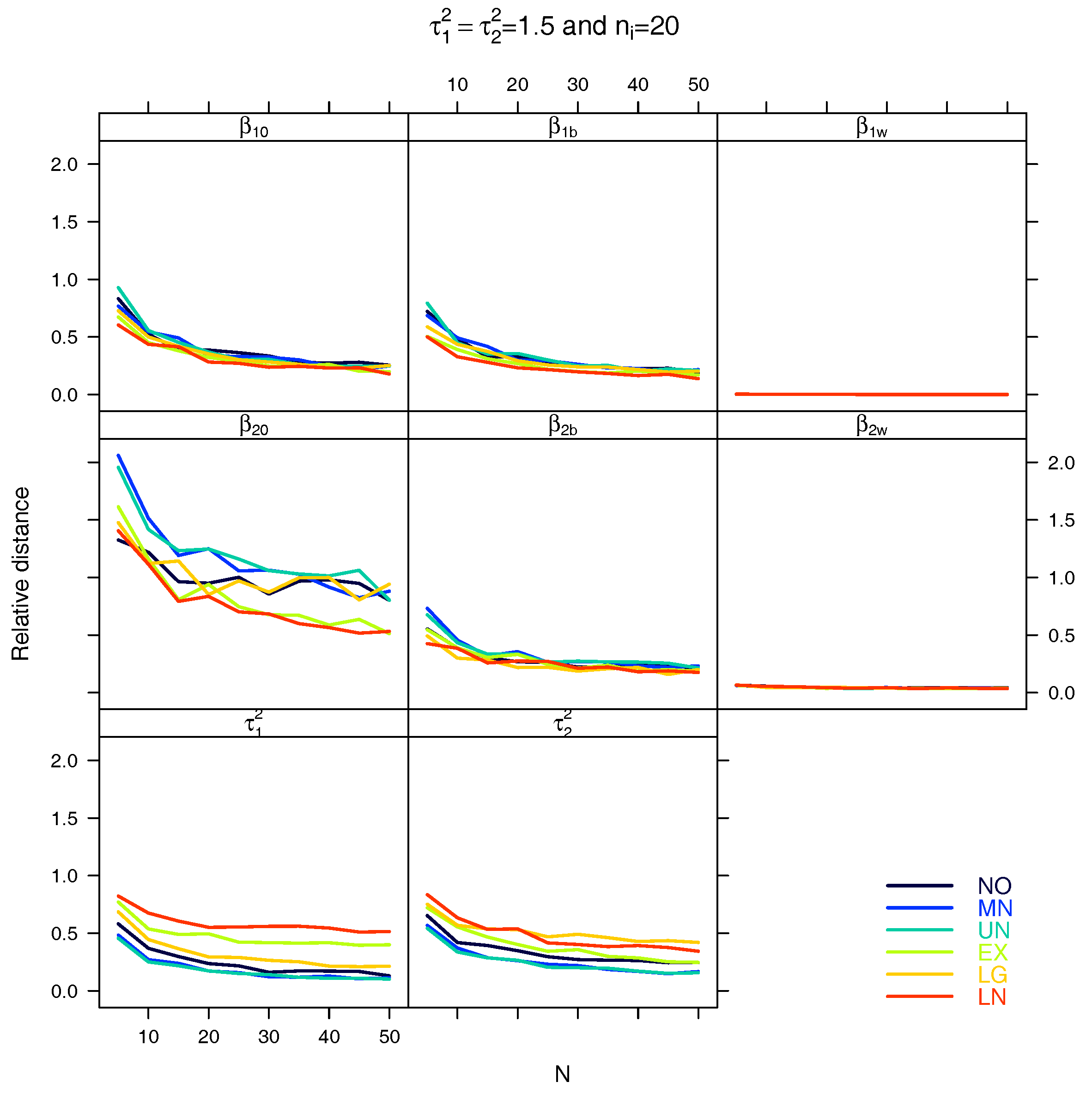
Figure A17.
Median of relative distance between and versus N for with and .
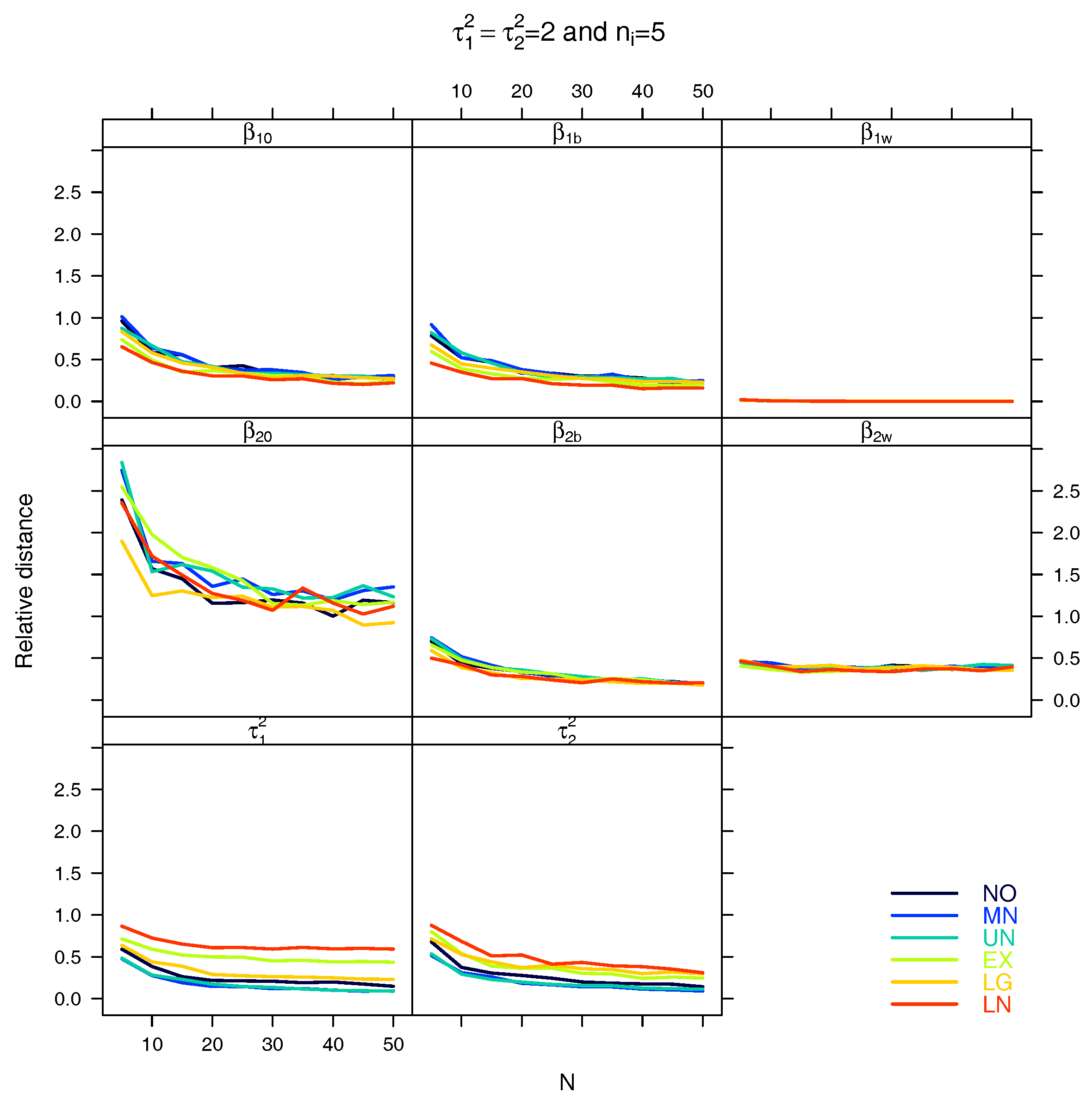
Figure A18.
Median of relative distance between and versus N for with and .

Figure A19.
Median of relative distance between and versus N for with and .
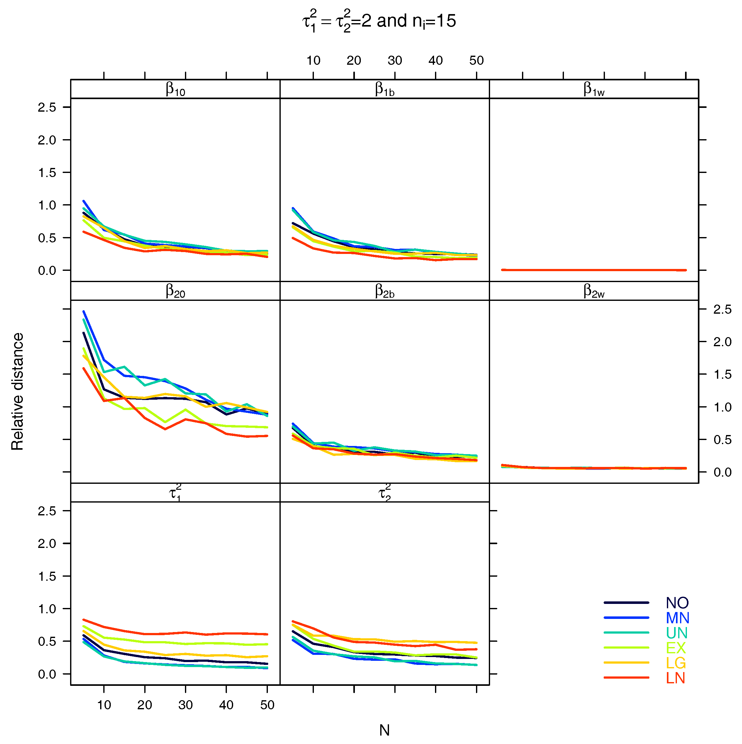
Figure A20.
Median of relative distance between and versus N for with and .
Next are the figures for Section 5.3.
Figure A21.
Median for the estimated fixed parameters for and .
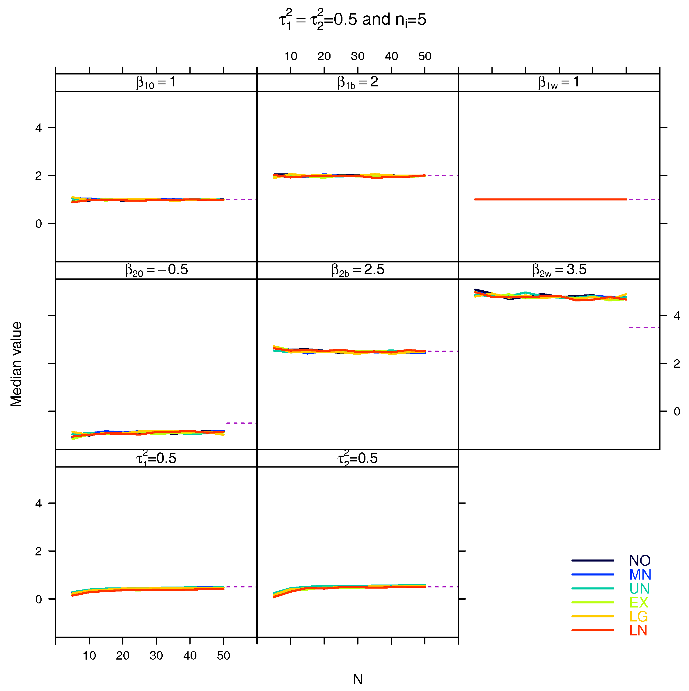
Figure A22.
Median for the estimated fixed parameters for and .
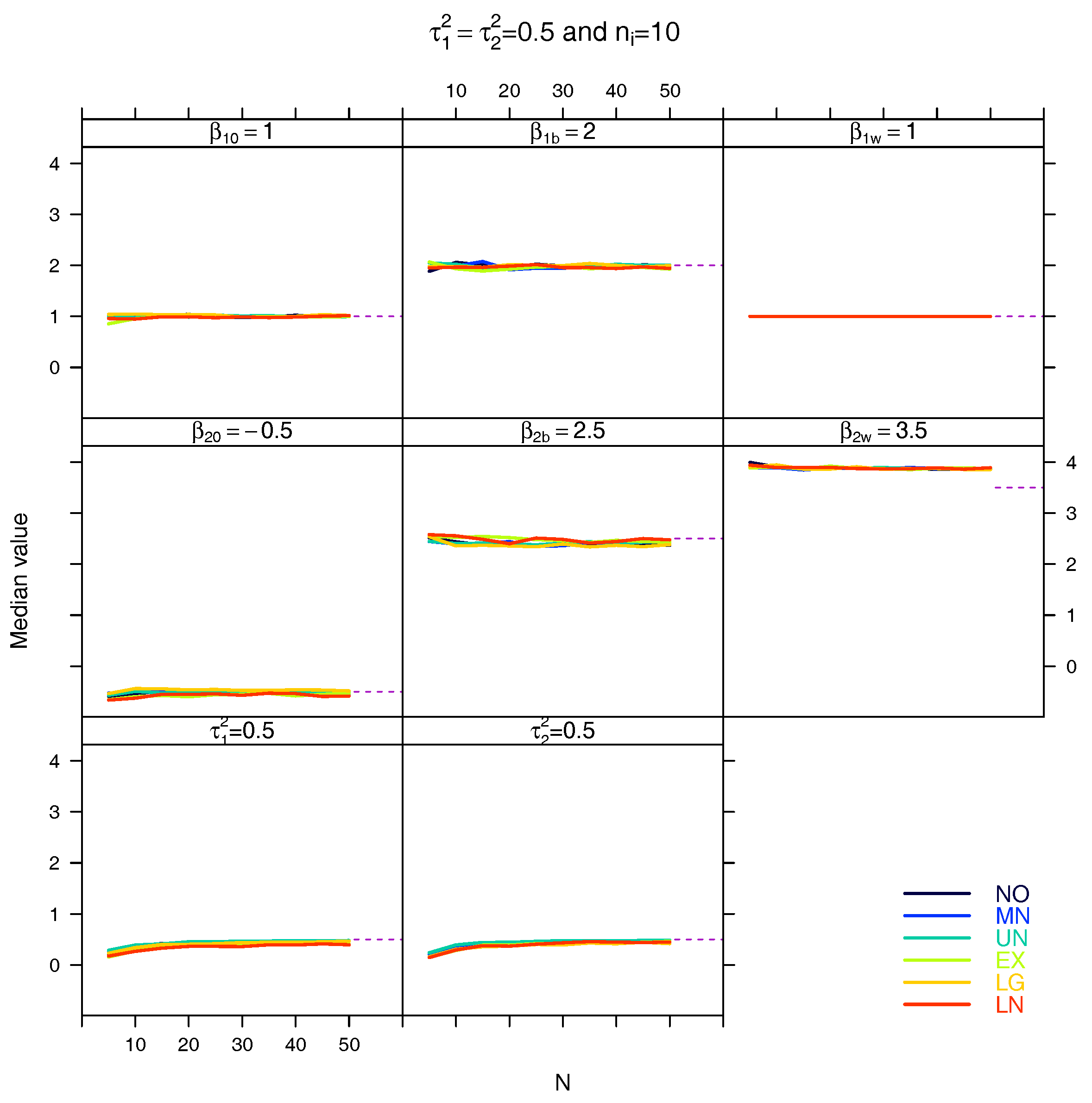
Figure A23.
Median for the estimated fixed parameters for and .
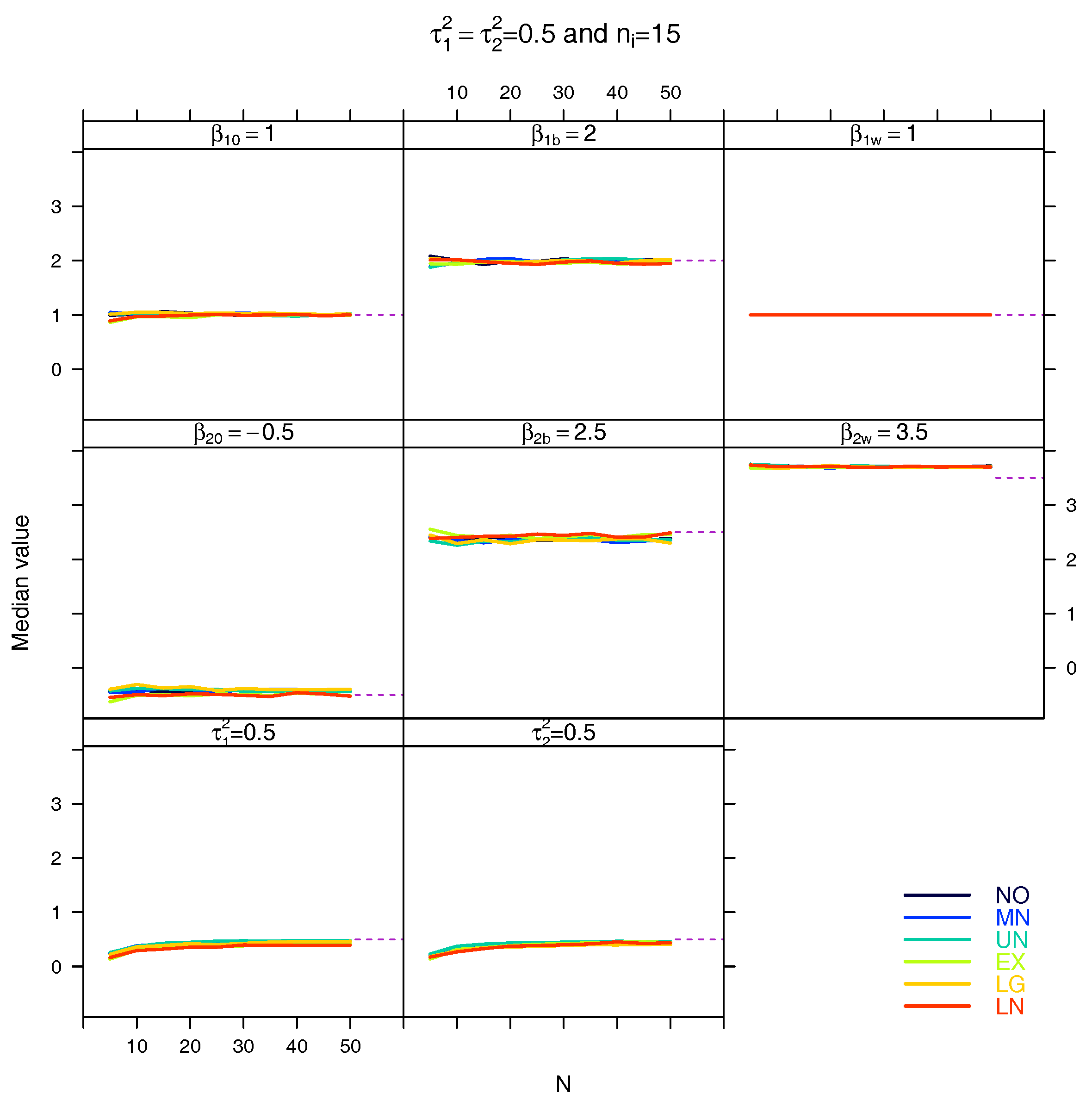
Figure A24.
Median for the estimated fixed parameters for and .

Figure A25.
Median for the estimated fixed parameters for and .

Figure A26.
Median for the estimated fixed parameters for and .
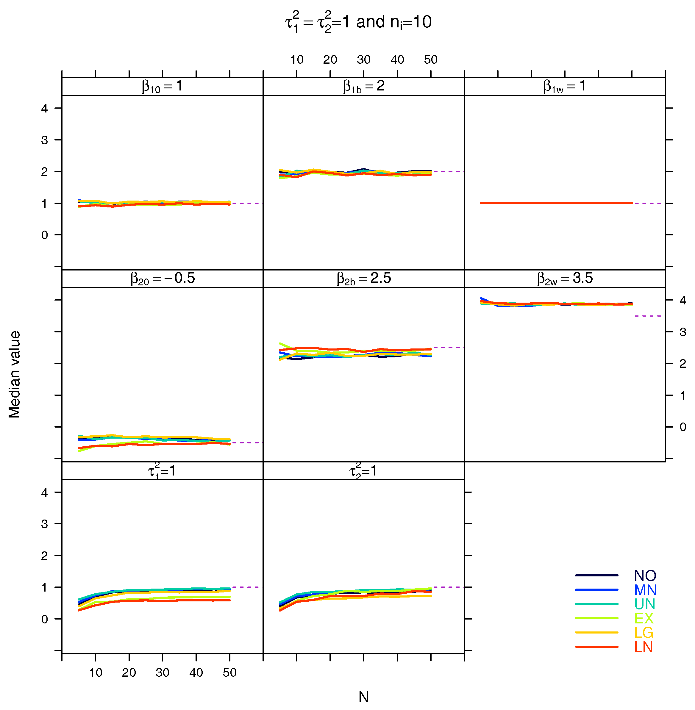
Figure A27.
Median for the estimated fixed parameters for and .

Figure A28.
Median for the estimated fixed parameters for and .
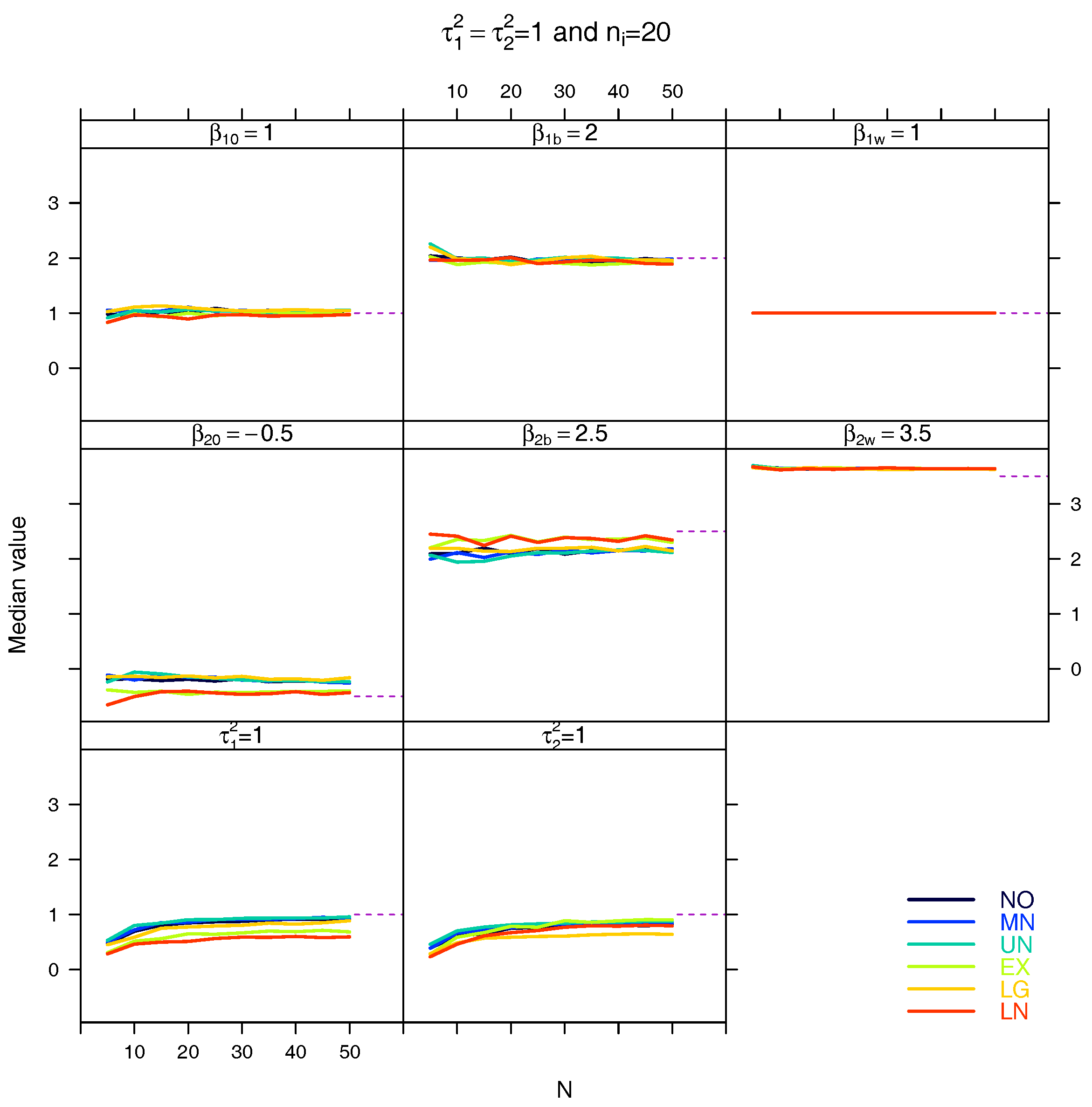
Figure A29.
Median for the estimated fixed parameters for and .
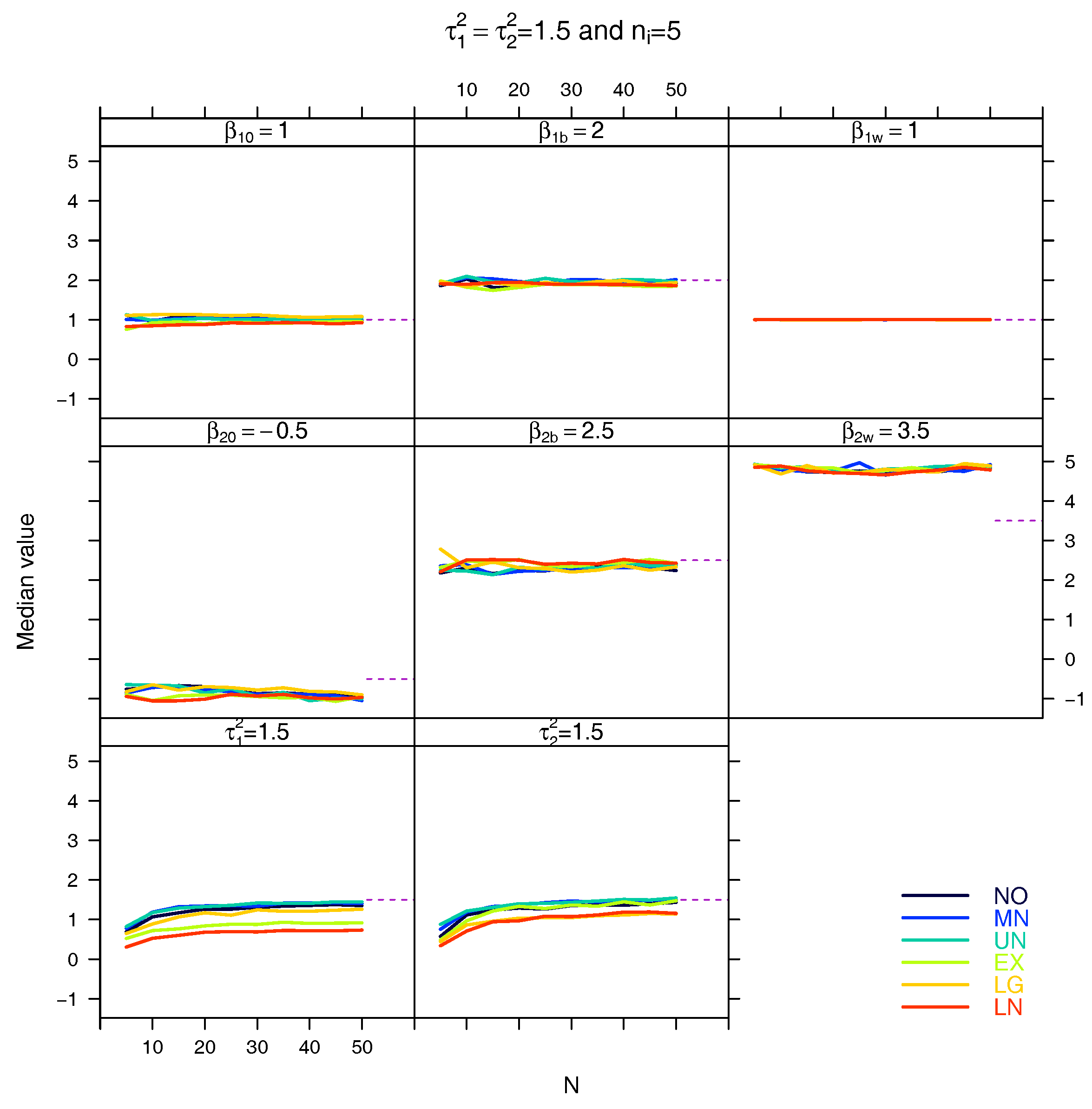
Figure A30.
Median for the estimated fixed parameters for and .
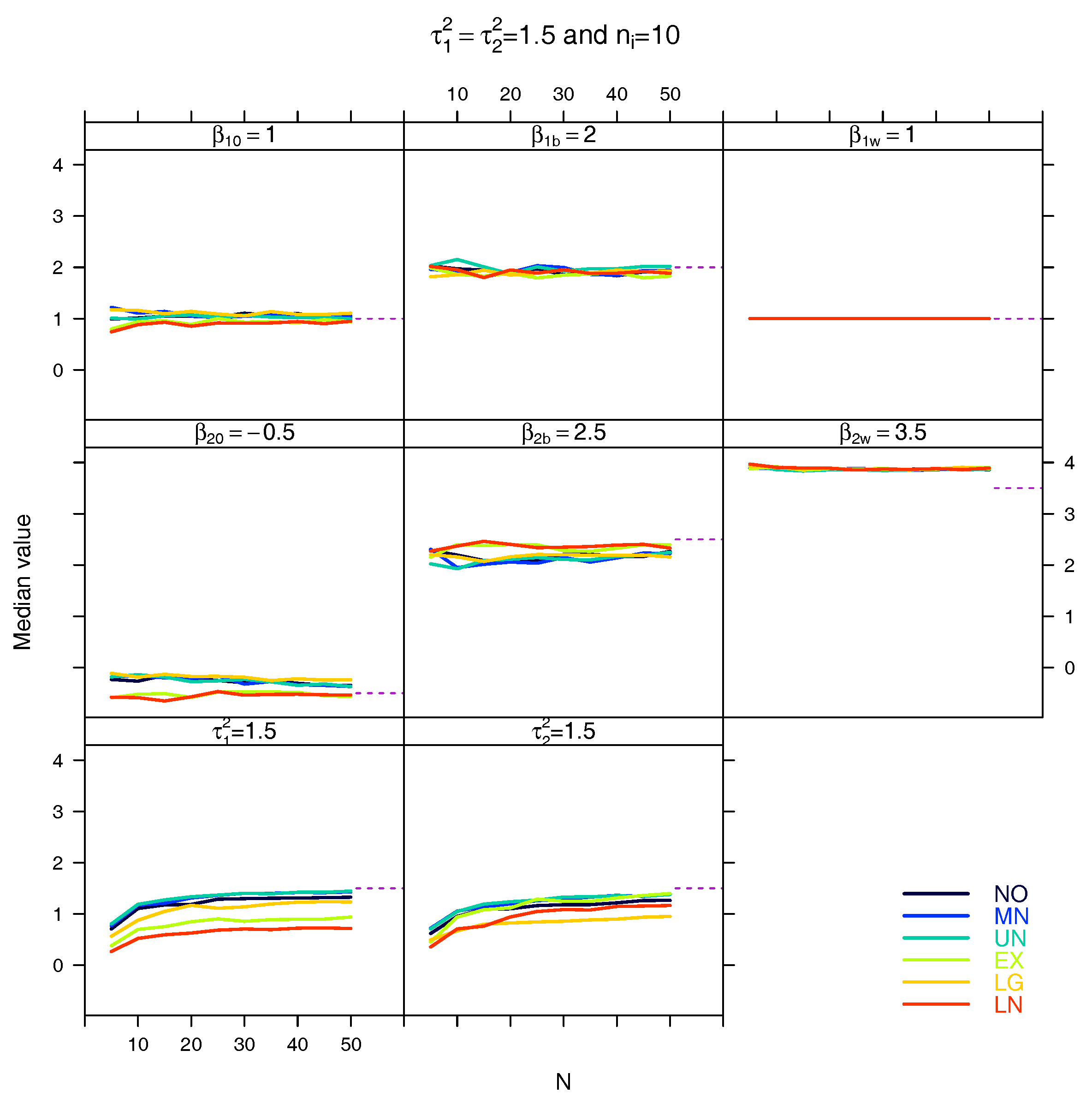
Figure A31.
Median for the estimated fixed parameters for and .
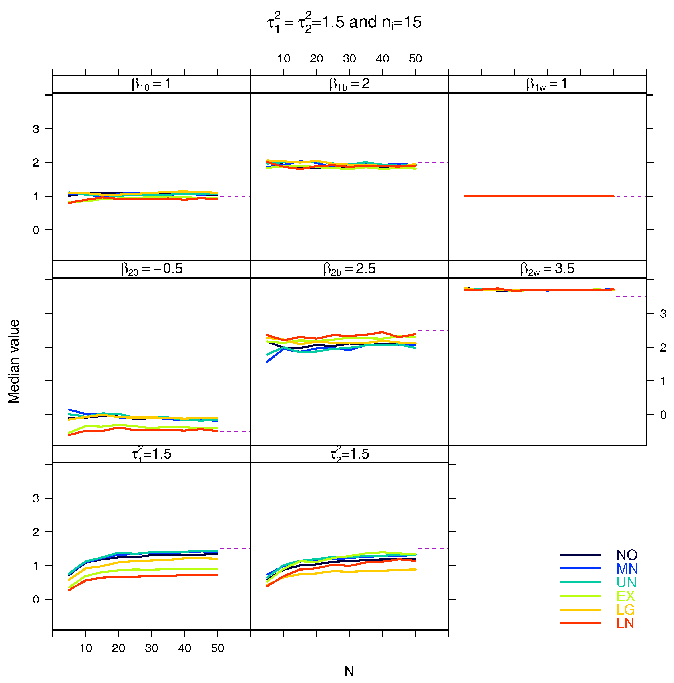
Figure A32.
Median for the estimated fixed parameters for and .
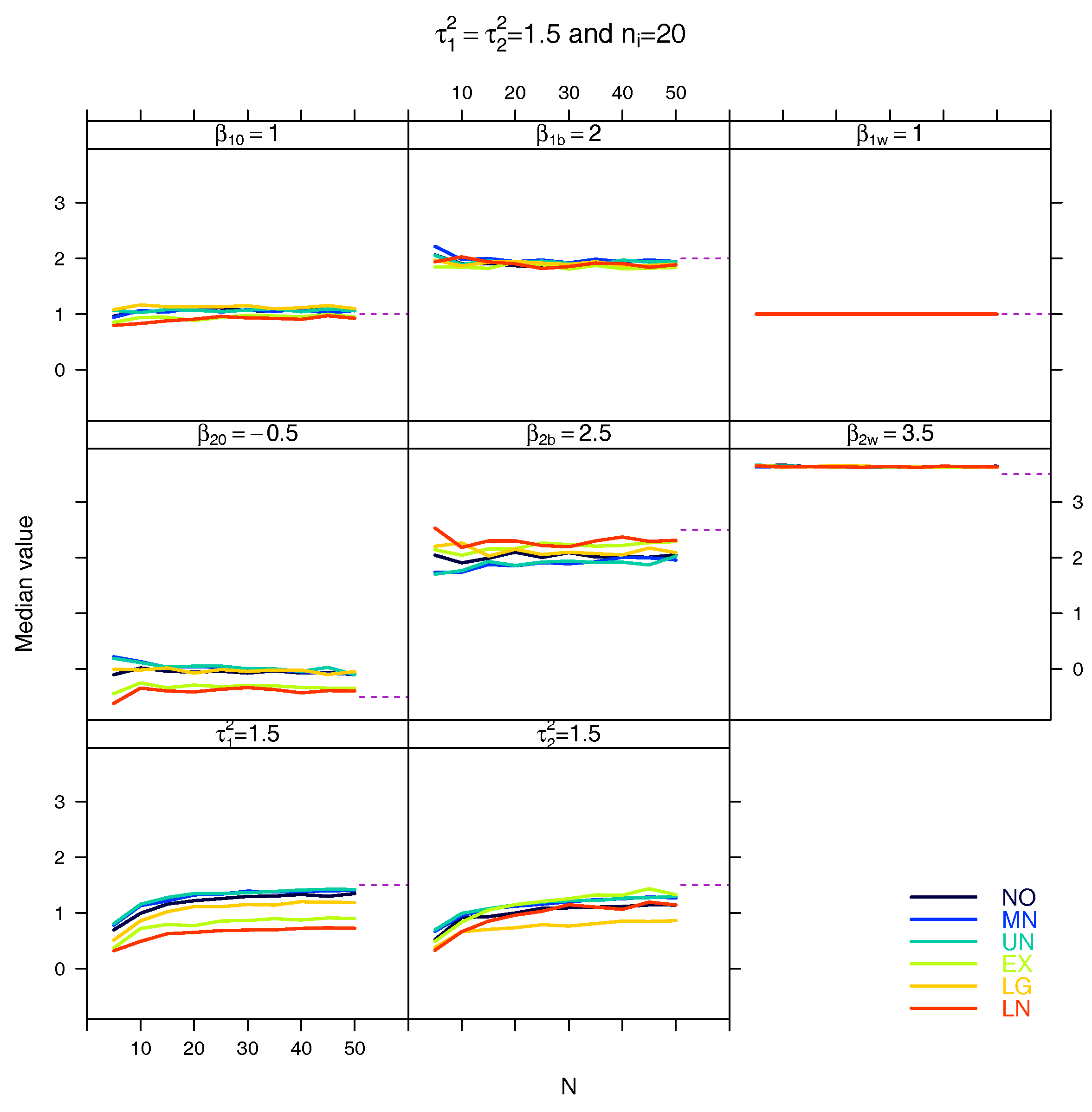
Figure A33.
Median for the estimated fixed parameters for and .

Figure A34.
Median for the estimated fixed parameters for and .
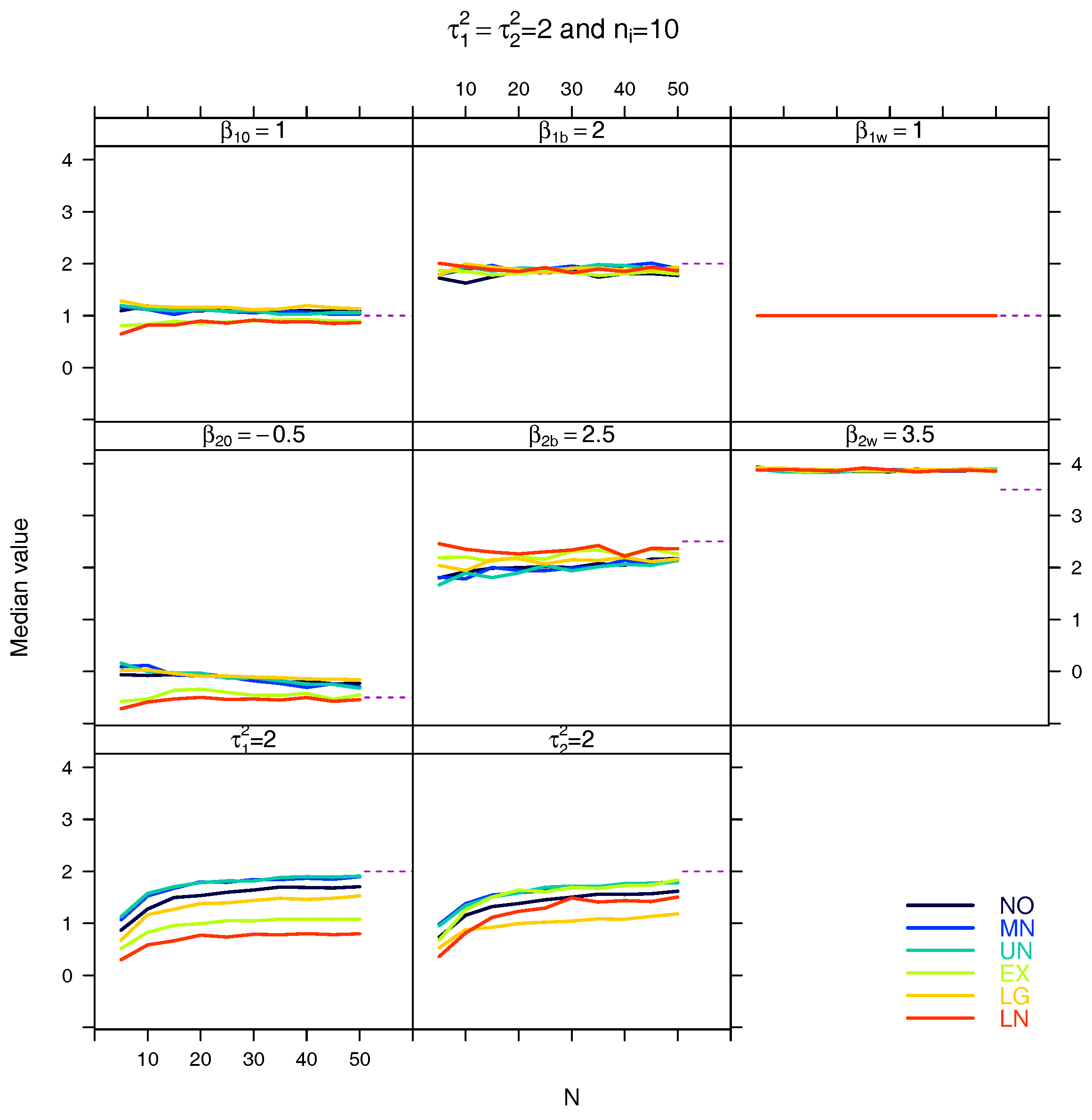
Figure A35.
Median for the estimated fixed parameters for and .
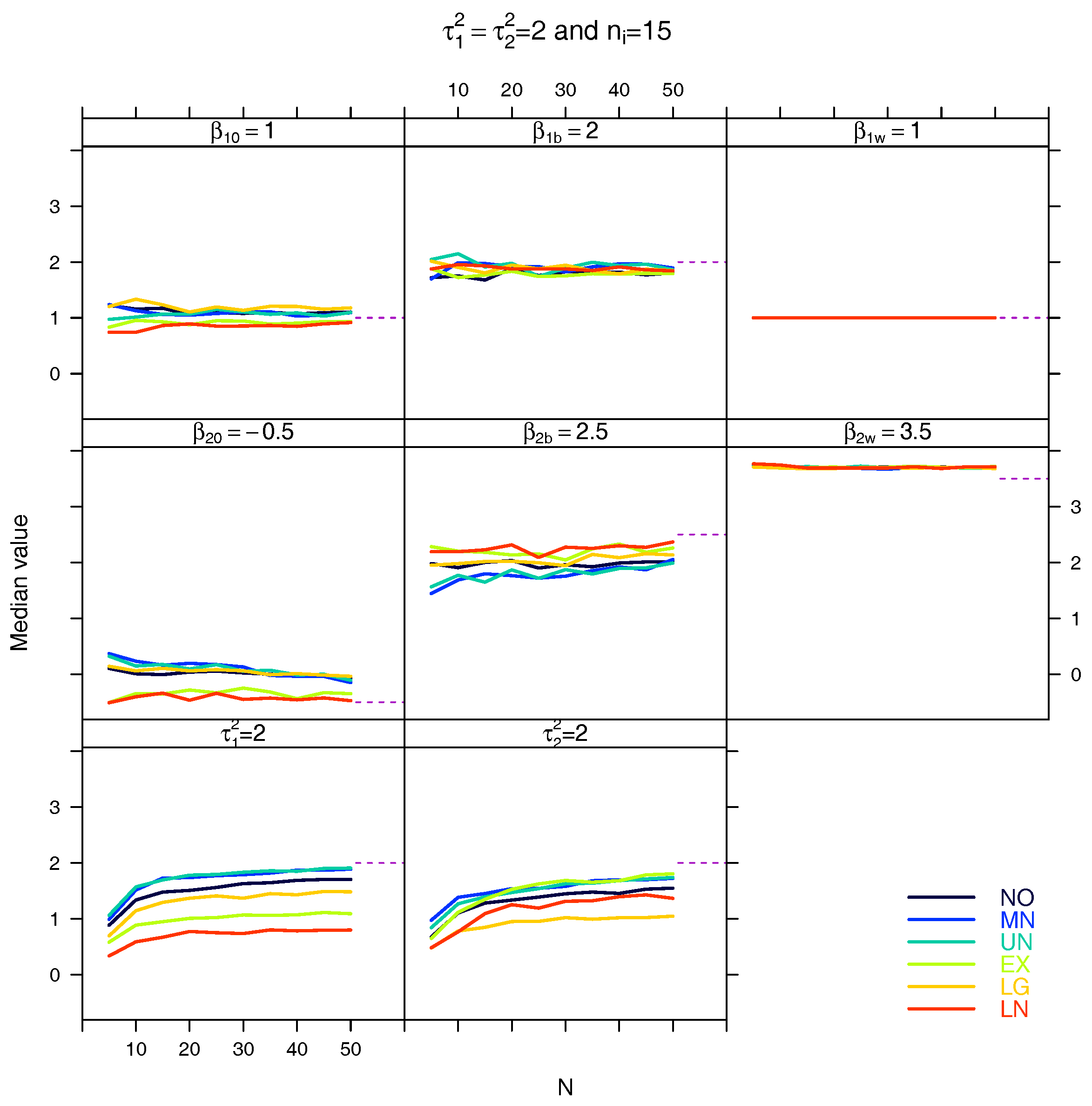
Figure A36.
Median for the estimated fixed parameters for and .
References
- Huang, X. Diagnosis of random-effect model misspecification in generalized linear mixed models for binary response. Biometrics 2009, 65, 361–368. [Google Scholar] [CrossRef] [PubMed]
- Neuhaus, J.M.; McCulloch, C.E. The effect of misspecification of random effects distributions in clustered data settings with outcome-dependent sampling. Can. J. Stat. Revue Can. Stat. 2011, 39, 488–497. [Google Scholar] [CrossRef] [PubMed]
- McCulloch, C.E.; Neuhaus, J.M. Misspecifying the Shape of a Random Effects Distribution: Why Getting It Wrong May Not Matter. Stat. Sci. 2011, 26, 388–402. [Google Scholar] [CrossRef]
- Verbeke, G.; Lesaffre, E. The effect of misspecifiying the random-effects distribution in linear mixed models for longitudinal data. Comput. Stat. Data Anal. 1997, 23, 541–556. [Google Scholar] [CrossRef]
- Neuhaus, J.M.; Hauck, W.W.; Kalbfleisch, J.D. The Effects of Mixture Distribution Misspecification when Fitting Mixed-Effects Logistic Models. Biometrika 1992, 79, 755–762. [Google Scholar] [CrossRef]
- Heagerty, P.J.; Kurland, B.F. Misspecified Maximum Likelihood Estimates and Generalised Linear Mixed Models. Biometrika 2001, 88, 973–985. [Google Scholar] [CrossRef]
- Agresti, A.; Caffo, B.; Ohman-Strickland, P. Examples in which misspecification of a random effects distribution reduces efficiency, and possible remedies. Comput. Stat. Data Anal. 2004, 47, 639–653. [Google Scholar] [CrossRef]
- Litière, S.; Alonso, A.; Molenberghs, G. Type I and Type II Error Under Random-Effects Misspecification in Generalized Linear Mixed Models. Biometrics 2007, 63, 1038–1044. [Google Scholar] [CrossRef] [PubMed]
- Litière, S.; Alonso, A.; Molenberghs, G. The impact of a misspecified random-effects distribution on the estimation and the performance of inferential procedures in generalized linear mixed models. Stat. Med. 2008, 27, 3125–3144. [Google Scholar] [CrossRef] [PubMed]
- Neuhaus, J.M.; McCulloch, C.E.; Boylan, R. A note on Type II error under random effects misspecifications in generalized linear mixed models. Biometrics 2011, 67, 654–660. [Google Scholar] [CrossRef] [PubMed]
- Litière, S.; Alonso, A.; Molenberghs, G. Rejoinder to “A Note on Type II Error Under Random Effects Misspecification in Generalized Linear Mixed Models”. Biometrics 2011, 67, 656–660. [Google Scholar] [CrossRef]
- McCulloch, C.E.; Neuhaus, J.M. Prediction of Random Effects in Linear and Generalized Linear Models under Model Misspecification. Biometrics 2011, 67, 270–279. [Google Scholar] [CrossRef] [PubMed]
- Neuhaus, J.M.; McCulloch, C.E.; Boylan, R. Estimation of covariate effects in generalized linear mixed models with a misspecified distribution of random intercepts and slopes. Stat. Med. 2013, 32, 2419–2429. [Google Scholar] [CrossRef] [PubMed]
- Fleming, R.A. The Weibull model and an ecological application: Describing the dynamics of foliage biomass on Scots pine. Ecol. Model. 2001, 138, 309–319. [Google Scholar] [CrossRef]
- Carroll, K.J. On the use and utility of the Weibull model in the analysis of survival data. Control. Clin. Trials 2003, 24, 682–701. [Google Scholar] [CrossRef]
- Abdel-Ghaly, A.A.; Attia, A.F.; Abdel-Ghani, M.M. The maximum likelihood estimates in step partially accelerated life test for the Weibull parameters in censored data. Commun. Stat. Theory Methods 2002, 31, 551–573. [Google Scholar] [CrossRef]
- Akaike, H. A new look at the statistical model identification. IEEE Trans. Autom. Control 1974, 19, 716–723. [Google Scholar] [CrossRef]
- Schwarz, G. Estimating the Dimension of a Model. Ann. Stat. 1978, 6, 461–464. [Google Scholar] [CrossRef]
- Lai, C.D. Generalized Weibull Distributions; Springer: Berlin, Germany, 2013. [Google Scholar]
- Murthy, D.N.P.; Xie, M.; Jiang, R. Weibull Models, 1st ed.; Wiley Series in Probability and Statistics; J. Wiley: Hoboken, NJ, USA, 2004. [Google Scholar]
- Rinne, H. The Weibull Distribution: A Handbook, 1st ed.; CRC Press: Boca Raton, FL, USA, 2009. [Google Scholar]
- Almalki, S.J.; Nadarajah, S. Modifications of the Weibull distribution: A review. Reliab. Eng. Syst. Saf. 2014, 124, 32–55. [Google Scholar] [CrossRef]
- Bagheri, S.F.; Samani, E.B.; Ganjali, M. The generalized modified Weibull power series distribution: Theory and applications. Comput. Stat. Data Anal. 2016, 94, 136–160. [Google Scholar] [CrossRef]
- Domma, F.; Condino, F.; Popović, B. A new generalized weighted Weibull distribution with decreasing, increasing, upside-down bathtub, N-shape and M-shape hazard rate. J. Appl. Stat. 2017, 44, 2978–2993. [Google Scholar] [CrossRef]
- Silva, G.O.; Ortega, E.M.; Cordeiro, G.M. A log-extended Weibull regression model. Comput. Stat. Data Anal. 2009, 53, 4482–4489. [Google Scholar] [CrossRef]
- Vigas, V.P.; Silva, G.O.; Louzada, F. The Poisson-Weibull Regression Model. Chil. J. Stat. 2017, 8, 25–51. [Google Scholar]
- Prataviera, F.; Ortega, E.M.; Cordeiro, G.M.; Pescim, R.R.; Verssani, B.A. A new generalized odd log-logistic flexible Weibull regression model with applications in repairable systems. Reliab. Eng. Syst. Saf. 2018, 176, 13–26. [Google Scholar] [CrossRef]
- Sohn, S.Y.; Yoon, K.B.; Chang, I.S. Random effects model for the reliability management of modules of a fighter aircraft. Reliab. Eng. Syst. Saf. 2006, 91, 433–437. [Google Scholar] [CrossRef]
- Sohn, S.Y.; Chang, I.S.; Moon, T.H. Random effects Weibull regression model for occupational lifetime. Eur. J. Oper. Res. 2007, 179, 124–131. [Google Scholar] [CrossRef]
- Bartolucci, A.A.; Bae, S.; Singh, K.P. Establishing a Bayesian predictive survival model adjusting for random effects. Math. Comput. Simul. 2008, 78, 328–334. [Google Scholar] [CrossRef]
- Lv, S.; Niu, Z.; Cui, Q.; He, Z.; Wang, G. Reliability improvement through designed experiments with random effects. Comput. Ind. Eng. 2017, 112, 231–237. [Google Scholar] [CrossRef]
- Stasinopoulos, M.; Rigby, B. gamlss.dist: Distributions for Generalized Additive Models for Location Scale and Shape. Available online: https://cran.r-project.org/web/packages/gamlss.dist/gamlss.dist.pdf (accessed on 30 May 2018).
- Pinheiro, J.C.; Chao, E.C. Efficient Laplacian and Adaptive Gaussian Quadrature Algorithms for Multilevel Generalized Linear Mixed Models. J. Comput. Graph. Stat. 2006, 15, 58–81. [Google Scholar] [CrossRef]
- Alonso, A.; Litière, S.; Molenberghs, G. A family of tests to detect misspecifications in the random-effects structure of generalized linear mixed models. Comput. Stat. Data Anal. 2008, 52, 4474–4486. [Google Scholar] [CrossRef]
- Alonso, A.; Litière, S.; Molenberghs, G. Testing for misspecification in generalized linear mixed models. Biostatistics 2010, 11, 771–786. [Google Scholar]
- R Core Team. R: A Language and Environment for Statistical Computing; R Foundation for Statistical Computing: Vienna, Austria, 2018. [Google Scholar]
- Drikvandi, R.; Verbeke, G.; Molenberghs, G. Diagnosing misspecification of the random-effects distribution in mixed models. Biometrics 2017, 73, 63–71. [Google Scholar] [CrossRef] [PubMed]
- Efendi, A.; Drikvandi, R.; Verbeke, G.; Molenberghs, G. A goodness-of-fit test for the random-effects distribution in mixed models. Stat. Methods Med. Res. 2017, 26, 970–983. [Google Scholar] [CrossRef] [PubMed] [Green Version]
Figure 1.
Empirical density function for time (left) and boxplot for time given each piece (right).

Figure 2.
Probability density function used for random effects, each one with zero mean and unit variance.
Figure 2.
Probability density function used for random effects, each one with zero mean and unit variance.


Table 1.
Parameter estimates, standard errors, p-values, and Schwarz Bayesian criterion () for the model (1).
Table 1.
Parameter estimates, standard errors, p-values, and Schwarz Bayesian criterion () for the model (1).
| Model for | Estimate | Std. Error | t-Value | p-Value |
| Intercept | 0.96 | 0.0065 | 149.1 | < |
| 1.80 | 0.0094 | 191.3 | < | |
| 0.99 | 0.0077 | 127.8 | < | |
| Model for | Estimate | Std. Error | t-Value | p-Value |
| Intercept | −0.64 | 0.1620 | −3.97 | 0.000125 |
| 2.69 | 0.2454 | 10.97 | < | |
| 3.62 | 0.2078 | 17.45 | < | |
| 486.46 | 560.93 |
© 2018 by the authors. Licensee MDPI, Basel, Switzerland. This article is an open access article distributed under the terms and conditions of the Creative Commons Attribution (CC BY) license (http://creativecommons.org/licenses/by/4.0/).
Share and Cite
MDPI and ACS Style
Hernández, F.; Giampaoli, V. The Impact of Misspecified Random Effect Distribution in a Weibull Regression Mixed Model. Stats 2018, 1, 48-76. https://doi.org/10.3390/stats1010005
AMA Style
Hernández F, Giampaoli V. The Impact of Misspecified Random Effect Distribution in a Weibull Regression Mixed Model. Stats. 2018; 1(1):48-76. https://doi.org/10.3390/stats1010005
Chicago/Turabian StyleHernández, Freddy, and Viviana Giampaoli. 2018. "The Impact of Misspecified Random Effect Distribution in a Weibull Regression Mixed Model" Stats 1, no. 1: 48-76. https://doi.org/10.3390/stats1010005