Building W Matrices Using Selected Geostatistical Tools: Empirical Examination and Application


Department of Spatial Econometrics, University of Lodz, POW 3/5 Street, 90-255 Lodz, Poland
Stats 2018, 1(1), 112-133; https://doi.org/10.3390/stats1010009
Submission received: 30 July 2018
/
Revised: 23 September 2018
/
Accepted: 26 September 2018
/
Published: 29 September 2018
Abstract
:This paper investigates how to determine the values (elements) of spatial weights in a spatial matrix (W) endogenously from the data. To achieve this goal, geostatistical tools (standard deviation ellipsis, semivariograms, semivariogram clouds, and surface trend models) were used. Then, in the econometric part of the analysis, the effect of applying different variants of matrices was examined. The study was conducted on a sample of 279 Polish towns from 2005–2015. Variables were related to the quantity of produced waste and economic development. Both exploratory spatial data analysis and estimations of spatial panel and seemingly unrelated regression models were performed by including particular W matrices in the study (exogenous-random as well as distance and directional matrices constructed based on data). The results indicated that (1) geostatistical tools can be effectively used to build Ws; (2) outcomes of applying different matrices did not exclude but supplemented one another, although the differences were significant; (3) the most precise picture of spatial dependence was achieved by including distance matrices; and (4) the values of the assessed parameter at the regressors did not significantly change, although there was a change in the strength of the spatial dependency.
1. Introduction
The construction of a spatial weight matrix (W) is an important problem of spatial econometrics [1]. This matrix considers and expresses the potential for interactions between pairs of observations in various locations [2]. The W matrix could be set a priori (W specified exogenously) by the researcher (e.g., [3,4]). On the other hand, it could also be estimated endogenously directly from the data [5]. Kooijman [1] was one of the first to explicitly tackle the question of estimating the W matrix endogenously. He suggested that weights could be built by maximizing the value of Moran’s I. His procedure aroused many doubts but provoked a search for innovative ways of solving the problem. For example, Lee [6] showed that the W k-nearest neighbor problem and other seemingly unrelated problems can be solved efficiently with the Voronoi diagram. In addition, Griffith [7] proposed finding weights in the W by absorbing spatial effects from the data. Additionally, Getis and Aldstadt [8] used the local statistical model and the AMOEBA algorithm (a multidirectional optimum ecotope-based algorithm). Fernández et al. [9] suggested a specification of W based on the measure of entropy. Later, Mur and Paelinck [10] focused on the maximization of the complete correlation coefficient. Stewart and Zhukov [11] indicted neighbors from the visualization of spatial effects, while Hondroyiannis et al. [12] and Keleijan and Piras [13] assumed that elements of W are an unknown function of two sets of exogenous variables. In addition, Benjanuvatra and Burridge [14] and Qu and Lee [15] presented the quasi-maximum likelihood estimator (QML) to estimate weights in W endogenously—directly from data. The selection problem of Ws is widely described in [4,8,16]. Specifications and estimation methods of models with an endogenous spatial weight matrix are widely presented in [15,17]. However, these issues are not within the scope of this research paper.
In this paper, an attempt was made to verify the research hypothesis that the selected methods and tools of geostatistics (the standard deviation ellipsis, semivariograms, and surface trend models) can be used to specify and develop values in a spatial weight matrix endogenously. This study also evaluates the effect of using different variants of spatial weight matrices on the results of exploratory spatial data analysis (ESDA) as well as econometric modelling, and identifies the differences that significantly occurred (over the space and in the time span). The analysis was conducted on a sample of 279 Polish cities from 2005 to 2015. Variables were related to the quantity of collected municipal mixed waste (it covers waste from households, including bulky waste, and similar waste from commerce and trade, office buildings, institutions, small businesses, yard and gardens, street sweepings, contents of litter containers, and market cleansing. Waste from municipal sewage networks and treatment and municipal construction and demolition is excluded [18]) and the economic development of cities (the value of the revenue of the city budget is in PLN per capita, Revenues). The ESDA, estimations of the spatial panel, and seemingly unrelated regression (SUR) models (with spatial error) were performed by including particular row-standardised spatial weight matrices in the study (exogenous as a random one and distance and directional matrices constructed endogenously based on the data). The research was conducted in ArcMap (by Environmental Systems Research Institute, ArcGIS), R (a free software environment for statistical computing and graphics), SAGA (a system for automated geoscientific analyses), and GeoDa (an introduction to spatial data analysis).
The paper is organized as follows. Section 2 presents the selected geostatistical methods used to specify and develop values in endogenous spatial weight matrices directly from the data. Semivariograms, based on which the spatial continuity (variation and degree of spatial correlation) of the specified phenomena can be effectively characterized depending on the distance, are introduced here as an effective tool in the construction of distance matrices. The standard deviation ellipsis and surface trend models are considered when the spatial tendency and directionality of the phenomena occurred and could be set in the Ws. To verify whether the application of spatial weight matrices differentiates the analysis results and to examine whether Ws should be different for different years the ESDA methods as well as the spatial panel model and seemingly unrelated regressions are applied. Moreover, the economic background of the analyzed scientific problem is also discussed in this section. Section 4 presents the outcomes considering the utility of applied tools and provides some ideas for evaluating the effect of using different spatial weight matrices on the modelling of the quantity of municipal waste in Polish cities. Some suggestions for further research are also published here. Conclusions are given in Section 5. Technical details are relegated to the appendix.
2. Selected Geospatial Tools in Weight Matrix Construction and Examination: Proposal
2.1. Semivariograms
Recalling Tobler’s first law of geography, the distance and neighboring relations between different areas can indicate to what degree spatial dependence exists and ‘how close places need to be’ to be related or spatially autocorrelated [19]. This law makes it clear that spatial relations are not static but evolve over distance.
In the structure of the spatial weight matrix based on the geographical distance, it can be difficult to determine the maximum distance to which units are autocorrelated (show similarity in terms of a studied feature resulting from mutual spatial relations). One of the main assumptions of the article is to describe and apply semivariograms based on which the spatial continuity (variation and degree of spatial correlation) of specified phenomena can be effectively characterized depending on the distance [20].
The variogram is defined as the variance (Var) of a random variable whose values are differences in the realization of the analyzed phenomenon in various locations of space D:
where are the realisations of a random variable in locations i and j, for i = 1, ..., N and j = 1, ..., N. In the variogram, each pair of spatial locations is considered twice. For this reason, to describe the differentiation of the variable depending on the distance of the measuring points, the semivariogram (semivariance) is commonly analyzed. Geostatistics determines it as half of the variogram:
The values of the semivariogram are distance functions and are not functions of specific locations. Therefore, the commonly used notation of the experimental (empirical) semivariogram is according to the classical formula proposed by Matheron [21,22] as follows:
with the constant mean assumption:
such that:
E[X(si + h) − X(si)] = E[X(si + h) − E[X(si)] = 0,
Var[X(si + h) − X(si)] = E[X(si + h) − X(si)]2 = 0.
Using h to mark the vector whose length may depend on both the distance separating two locations and, in some cases, on the direction of measurement and which is an independent variable of the function of the experimental semivariogram, one may use the following formula (unlike a correlation coefficient, semi-variance is not normalised, and values are not constrained like most correlation measurements [23]):
and (6) may be estimated by:
where is the number of pairs of experimental data separated by the distance . In the case of an isotropic process of the random field, arguments of the semivariogram function do not depend on direction: . According to the graphical representation of the semivariance from the data, when analyzing changes in values of the semivariogram with changing distance, one may distinguish the spatial variability (dependence) of the process. Semivariance values range between 0, which indicates complete autocorrelation, and , which indicates complete randomness in the data. It is a way to obtain an estimate of the general range of spatial dependence, which can be fitted to the theoretical semivariogram that can also be used as a model for spatial interpolation (kriging) [21]. One can use a variety of permissible theoretical semivariogram models for the fitting procedure (i.e., exponential, Gaussian, power, spherical, cubic, sine hole effect, penta-spherical, matérn class); see, e.g., [24] or [25]. However, the idea of spatial interpolation is not the aim of this paper. The theoretical semivariogram is a plot, in which the values should increase as the distance increases until they reach a ‘sill’, which is the maximum level of γ(h) on the y-axis. The distance to the sill on the x-axis is called the ‘range’ (α0). The range of distance h from zero to the point at which the semivariogram attains approximately 95% of the constant value is called the effective range—the range that expresses the longest distance at which the values of the semivariogram are still correlated. With a further increase in the distance, autocorrelation can no longer be observed. Finally, the nugget (c0) effect can be attributed to measurement errors or spatial sources of variation at distances smaller than the sampling interval or both. Measurement error occurs because of the error that is inherent in measuring devices. Natural phenomena can vary spatially over a range of scales. Variation at micro scales smaller than the sampling distances will appear as part of the nugget effect [26] (Figure 1).
With a lack of spatial autocorrelation of the analyzed phenomenon, the semivariogram takes the form of a line parallel to the horizontal axis. Step changes show that the variable is not continuous and has highly irregular spatial variability (directionality). If the analysis of the phenomena is characterized by a specific pattern of spatial similarities, then the semivariogram may be a function of increasing and decreasing variable values that depend not only on the distance but also on spatial directions. It is called the directional semivariogram and constructs individual semivariograms arranged by direction [28] (pp. 34–51).
2.2. Standard Deviational Ellipse
The directionality of the phenomena, indicated by the semivariogram cloud (it displays the individual point-pair contributions to the final semivariogram. When compared with the simple semivariogram, it allows a subjective impression to be gained of whether the apparent pattern of spatial variation is related to systematic trends in the data or to a few unusual points [29]), may also be confirmed by the standard deviational ellipse (SDE; Figure 2).
Standard deviation arises as one of the classical statistical measures for depicting the dispersion of univariate features around the center. Its evolution in two-dimensional space arrives at the SDE, which was first proposed by Lefever [31] in 1926. Ever since then, SDE has long served as a versatile geographical information system (GIS) tool for delineating the bivariate distributed features. It is typically employed for sketching the geographical distribution trend of the relevant features by summarizing both their dispersion and orientation. Therefore, it has also been adopted to quantitatively analyze the orientation anisotropy [32]. The SDE is mainly determined by three measures: average location, dispersion (or concentration), and orientation [33]. What is crucial is that one can calculate the SDE using either the locations of the features or using the locations influenced by an attribute value associated with the features. The latter is termed “a weighted SDE”. Here, this was used to determine the directionality of the variable. Then, the trend surface analysis was applied to prove the anisotropy and to indicate the values of the directional matrix. The standard deviational ellipse calculation may be based on an optional ‘weight field’ (to obtain the ellipses for locations weighted by Waste, for example). This numeric field is used to weight locations according to their relative importance [34].
2.3. Trend Surface Analysis
The trend surface analysis (TSA) describes trends of changes of a phenomenon in a geographical space and, consequently, enables one to come to conclusions concerning agglomeration, dispersion, or spatial global trends and local fluctuations [35]. The TSA is one of the global surface-fitting procedures (i.e., spatial trend identification supporting inference about the nature of the spatial trend estimation of a phenomenon) and one of the oldest mathematical analytical methods used for spatial non-stationarity analysis. The TSA parameters reflect the strength and direction of global and local trends (i.e., systematic heterogeneity of a phenomenon expressing itself with the mean of a spatial process). A random component enables one to grasp the variability of a phenomenon of the mean constant in space, which makes identification of the potential spatial relations possible. According to Chojnicki and Czyż [35], the TSA method enables one to provide a simplified description of a spatial process of high complexity by means of separating large-scale systematic spatial changes from small-scale local fluctuations. Depending on the spatial structure, variability, and nature of a phenomenon, spatial (surface) trend models take different forms of a function (from linear to a polynomial of any degree).
However, one should note that these models do not provide information on the causality of a phenomenon in space. Regarding the estimation of regression of a specific dependent variable (zij), where independent variables in the basic version of the model are orthogonal geographic coordinates (Xcoori, Ycoorj), the estimation of the model gives an answer to the question regarding whether there are any principles governing the spatial distribution of the analyzed phenomenon in the defined geographical area [35]. Depending on the nature of spatial changes of the phenomenon, one may discuss a linear spatial trend (8) or non-linear spatial trend estimation, for example, expressed by means of a second-degree polynomial, higher n degrees, and analogous versions of models with an added set of independent variables. The general form of linear TSA is as follows:
where zij is a dependent variable in a geographical space, Xcoori, Ycoorj are independent variables (flat coordinates of geographic location), α0 denotes the constant, absolute term and represents the height of the surface at the map origin where Xcoori = Ycoorj = 0 [36] (p. 6), α1, ..., αi are the structural parameters standing near flat coordinates, and εij is a random component.
In the surface trend model, the signs of estimates of parameters are subject to estimation. ‘Interpretation’ of the value makes sense when comparisons are made over time. The sign of the estimate of the parameter next to variable Xcoori describes the global trend of the phenomenon from the west to the east of the area, while the sign of the estimate of the parameter next to the variable Ycoorj provides information on the global trend from the south to the north. The remainders obtained from the surface trend model give a picture of the local fluctuations and deviations—the so-called spatial local trends—that are specific to a certain unit. The weights in the matrix were given in such a way that the units of a clearly stronger directional spatial trend were attributed with higher values. On the other hand, the outliers, which clearly stand out regarding the level of the analyzed phenomenon, were attributed with the highest weights in relation to their values.
The above-mentioned methods were used to give the values of weights in endogenous Ws. The matrices were row-standardized—this means that each element in the -th row is divided by the row sum. The elements of the row-standardized matrix take values between zero and one. The sum of the row values is always one [2,17]. On the other hand, to determine whether varied values of spatial weights lead to significant differences in the analytical results and to determine the results if we introduce a weight matrix built without considering the nature of phenomena, five spatial weight matrices were introduced to exploratory spatial data analysis (ESDA) as well as panel and seemingly unrelated regression (SUR) models to examine whether weight matrices should be different for different years.
2.4. ESDA and Spatial Models
The exploratory spatial data analysis is the latter set of methods that allow for the study and understanding of the spatial distribution and spatial structure as well as the detection of spatial dependence or autocorrelation in the data [7]. The most common spatial autocorrelation indicator in the literature is Moran’s I [37]. The global and local statistics of Moran were used, first, to examine the spatial interactions in the analyzed phenomena and, second, to compare the effects of applying different variants of matrices on the spatial dependencies.
Moreover, the spatial econometric models with spatial autocorrelation of the error component (spatial panel [38,39] and spatial SUR [40]) were applied. First, this was to check whether the results are sensitive to a change in the matrices, second, to verify whether the modelling results are substantially accurate, and the application of different Ws is justified, and finally to verify whether using the different matrices has an influence on the general stability of models over time. If a weighting matrix in a spatial model is endogenous, typical model specifications will no longer be appropriate. Similarly, regression parameter estimators that do not account for the endogeneity of the weighting matrix will typically be inconsistent. To avoid problems with misspecifications or the method of estimation, spatial error models were applied rather than autoregressive models [13].
The fixed-effects panel model with spatial autocorrelation of the error term is as follows:
where is the vector of dependent variables, consisting of one observation on the dependent variable for every unit in the sample = (y1t, ..., ynt)’. In addition, is the vector of disturbance terms, and is the matrix of independent variables, where . The is the vector of dummy variables introduced for each spatial unit as a measure of the variable intercept, . The is the vector of parameters, and λ is the spatial autocorrelation coefficient. Moreover, Wm is the matrix of spatial weights n × n, where m = (1, ..., 5), and is the vector of independent error terms, obeying the normal distribution for , and n denotes the number of units (number of cities where n = 1, ..., 279).
A spatial SUR with spatial autocorrelation of the error component (SUR-SEM) is as follows:
where γt denotes the vector of parameters, is the vector of disturbance terms, is the vector of independent error terms, and λ is the vector of spatial autocorrelation coefficients. The remaining variables are as defined in Equation (9).
To specify and develop values in endogenous spatial weight matrices, the selected methods and tools of geostatistics will be used. To test the statistically significant spatial relationships among cities, to examine whether the strength of these interactions changes with distance, and to verify whether the application of spatial weight matrices differentiates the analysis results, the ESDA methods will be applied. Furthermore, to determine whether varied values of spatial weights lead to significant dissimilarities in the economic results, the spatial panel with an error term model will be introduced. Finally, to examine whether weight matrices should be different for different years, considering the character of the data, any spatial heterogeneity underlying in the variables and the effect of any relevant unobservable variable the SUR-SEM will be used (with each equation corresponding to a year of analysis).
3. Results
3.1. Spatial Weight Matrices
3.1.1. Geographical Distance
Distances from the geographic centers of Polish cities, which served to build three spatial weight matrices, were selected based on the statistically significant spatial relationships characterizing the discussed phenomenon—the quantity of produced waste in kilograms per capita (averaged for 2005–2015) in 279 Polish towns (Wasteav). Preliminarily, to evaluate the scope of the spatial autocorrelation (similarity) and to show the semivariance values of specific ranges of distances among the compared pairs of locations, the empirical (experimental) semivariogram was calculated and drawn (the systematic first-order trend was removed); see Table 1 and Figure 3. Moreover, to indicate the ‘effective’ range from which the data became the most spatially independent, the empirical model was fitted to the theoretical one (see Figure 3 and Table 1). The omnidirectional stable semivariogram model was the most optimal in terms of the parameter values (nugget, range, partial sill, and sill), and it had the lowest mean squared and standard errors [20] or [25] (p. 25). In ArcGIS, the geostatistical analyst extension tool was used to construct the stable semivariogram model for the studied phenomena using ordinary kriging. Several other types of semivariogram models (circular, spherical, exponential, Gaussian, etc.) were examined; however, the stable model fitted the data best (all results of the modelling available by email).
The data shown in Table 1 and Figure 3 indicate that, for the individual distance ranges, the spatial autocorrelation characterizing the municipal waste collection in Polish cities on average reached 21 km, 57 km, 177 km, 263 km, 290 km, 347 km, and 545 km (values of the semivariogram decreased with distance periodically). The length of 545 km indicates the ‘effective’ distance of the semivariogram from which there is no significant spatial autocorrelation in the data.
To summarize, the results of this part of the analysis indicated that waste collection (management) might be local (regional, social, and urban economic development and waste policy determine the volume of waste streams) and global in nature. Spatial autocorrelation reached more than 500 km, undoubtedly due to the transboundary shipment of waste [41]. Hence, three matrices were built for selected geographic distances: W1—a weight matrix built based on the close distance from the determined geographic centers of cities with a radius of up to 57 km; W2—where the weights were determined depending on the ‘medium’ geographic distance from the geographic center of the city and units contained in a radius of up to 263 km, and W3—based on a radius of up to 545 km (long-distance weight matrix).
3.1.2. Directional Matrix
Examining the semivariogram clouds (Figure 4), it appears that, on average, there are differences in the semivariance values of the amount of the collected waste in Polish cities depending on direction. Changing the direction, as shown in Figure 4, some linked locations have values that finally result in higher semivariogram values. This indicates that cities separated by a selected distance of about 230,000 m in the northwest direction are on average more diverse and higher in terms of waste streams than locations in the south and east. As a result, these semivariogram clouds that present the correlations of spatial variability show that the variability varies not only with distance but also along with spatial directions; this is called ‘anisotropy’.
Considering the assumption of the anisotropy in spatial autocorrelation (Figure 4), the asymmetrical directional matrix was built (W4), based on the ‘medium’ geographic distance matrix W2. The weight values were initially determined based on the slope (orientation) of two SDEs, weighted by Wasteav. (Figure 5), and then were made more precise and confirmed by assessments of the parameters of the linear spatial trend model (TSA; Equation (8)).
The dependent variable in the estimated trend model was the waste quantity in Polish cities averaged by years. The form of the model is given by the following formula:
where Wasteav. is the averaged quantities of mixed waste collection in kilograms per capita; Xcoor and Ycoor are the standardized geographic coordinates of the centers of the analyzed Polish cities; β0, β1, and β2 are the structural parameters of the model; and is a random component. After assessing the parameters, the model takes the following form:
Not all estimated parameters of Model 12 were statistically significant at the assumed significance level of α = 0.05 (for critical value t* = 1.65, df = 276). They confirmed only the presence of a surface trend in waste collection (west–east). Signs of assessed parameters at the X coordinate were negative (−189). This indicated a downward spatial trend in the west–east directions (confirmation of the initial assumptions read off the SDE (Figure 5). Therefore, cities in western Poland were characterized by a higher level of the analyzed variable, and there was a downward trend among cities in the eastern parts of the country.
Based on the information about spatial trends in the average amount of collected municipal waste in Polish cities from 2005 to 2015, a spatial weight matrix was built. The matrix considered the occurrence of the spatial trend in such a way that cities in north-western Poland were assigned higher weights, from 3 to 4, reflecting an upward spatial trend (compare Figure 5), whereas central and eastern cities were assigned lower weights, from 1 to 2. Moreover, while analyzing the local spatial trends (Equation (12), high outliers were observed where volumes of waste exceeded the average for the studied Polish cities. In matrix W4, a weight of 5 was assigned to those cities. The cities were Sopot, Karpacz, Augustów, Lidzbark, Legnica, Szczawnica, Karpacz, Sławków, and Zakopane (Figure 5). The analysis indicated the TSA model defined by Equation (12) as the best under the formal regimes: Jarque–Bera = 5.99 with p = 0.37, Breusch–Pagan = 3.66 with p = 0.18, and lower values of Akaike and Schwarz rather than models with high levels of function values.
It can be inferred from Figure 5 that the directions of the intensity of waste production in Poland are south-west and central-north. The flattening of the weighted ellipse of two standard deviations (which contains ~95% of observations) indicates a certain spatial trend in waste streams in Polish cities, which is made more precise and confirmed by statistically significant assessments of the surface trend model parameters.
3.1.3. Random Weight Matrix
This matrix (W5) was set a priori (specified exogenously). The nearest neighbor matrix was built, which is based on the adjacency of the eight nearest cities (the only explanation might be that the average number of city neighbors was eight—without considering the content of the data).
3.2. ESDA
At this stage of the study, I seek an answer to the research question of whether the volume of municipal waste in Polish cities shows statistically significant spatial relationships. Does the strength of these interactions change with distance? Does the application of spatial weight matrices differentiate analysis results, and are they justified and factually correct?
The results of the ESDA analysis indicate the presence of significant and varied interregional relationships, which are different for specific years of the study and by the type of W matrix (Table 2).
When applying all spatial weight matrices, positive and statistically significant global Moran’s I statistic values were obtained. This means that, during 2005–2015, the cities displayed a tendency to cluster in space with respect to a similar volume of collected municipal waste. The strongest relationship characterized the amount of mixed collected waste for adjacency as defined by the matrix of close distance W1 and directional matrix, W4. On average and in the selected years, stronger positive and statistically significant spatial interactions also characterized volumes of waste in cities located close to each other, rather than in cities far away from one another. Moreover, data contained in Table 2 indicate that the strength of statistically significant spatial relationships decreased from 2005 to 2015 (an average flow of 57% in Moran’s I statistic value in 2015 as compared to 2005). Thus, the production and management of waste in a city still significantly affects the volume of that phenomenon in its adjacent units; however, these processes seem to be more condensed (e.g., due to the new thermal waste treatment plants or a more effective local waste management policy) [41]. Overall, the results obtained from global autocorrelation indicate statistically significant differences in strength, especially between results provided with W3 and W4 as well as with W3 and W5 (Kruskal–Wallis post-test, Dunn’s multiple comparison test). In the local indicators of spatial autocorrelation processes, results from ESDA using this matrix appear more precise and more specific because the values of global spatial autocorrelation are conditioned by local spatial regimes. Figure 6 shows the local indices of spatial autocorrelation determined based on matrices W1, W2, W3, W4, and W5.
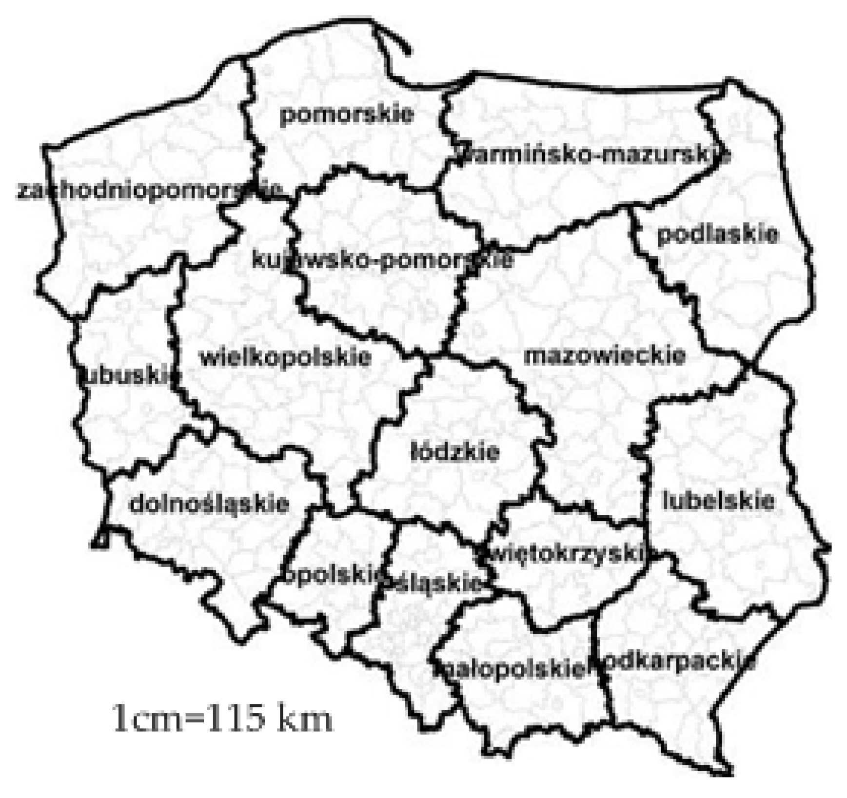
According to Figure 6, the general pictures of spatial relations characterizing the annual amounts of collected mixed municipal waste are similar, regardless of the spatial weight matrix included in the analysis. Namely, between 2005 and 2015, the cities located in western Poland were characterized by high-level variables and created classes of similar values. On the other hand, in the units located in the eastern part of the country, in the selected voivodeships in east-southern Poland and in Mazowieckie Voivodeship, the annual amounts of collected municipal waste are smaller than in other parts of the country (for a map of Polish voivodeships, see Figure A1). Such a situation may relate to higher urbanization rates and levels of economic development of cities in western Poland as well as to the higher level of ecological awareness [42]. On the other hand, the observation of the phenomenon behavior near Warsaw, which is the capital of Poland and one of the wealthiest cities in the country, demonstrates that the amount of annual waste is related to the ‘wealth’ of a city (i.e., higher levels of consumption, population density, investments, some issues related to ecology and environment, and the level of development of a city).
The most precise, detailed, and substantial picture of the occurring spatial relations was obtained by including the matrix of close distance (of a radius up to 57 km), spatial trend, and long distance (up to 545 km). The analysis of relations with the use of properly designed distance matrices revealed the occurrence of many specific units, the so-called outliers, in intercity relations (especially high-low, e.g., the cities that have a high amount of waste are surrounded by locations that have a lower level of the phenomena). These matrices indicated on some mechanisms that could be the reason the spatial heterogeneity exists in the amount of municipal waste among Polish cites. First, in Mazowieckie, there are relatively large differences between provinces or cities that are mainly due to population density and the degree of the industrialization of urban areas (especially Warsaw) [43]. Second, according to the Polish local database, in the eastern parts of the country, there is a strong concentration of illegal dumping sites, from which tons of municipal waste were collected while closing them down. Moreover, the regions situated in the east of Poland are those where the economic development is faster than in the rest of areas, mostly through the European Regional Development Fund between 2007 and 2013. Finally, those spatial matrices detected regions of southern Poland that are attractive for tourists and therefore generate a high increase of waste.
That cannot be said when one estimates the results obtained by including the randomly defined spatial weight matrix. The picture of local relations obtained based on the randomly generated matrix is poor. The scale of the detected statistically significant spatial relations with the use of matrix W5 is significantly different from the scale of the revealed urban settlements playing a part in spatial processes with the use of other matrices, defined a priori.
Generally, the W4 and W5 matrices emphasize the strong clusters of the most and least waste productive cities and stress the role of these urban areas on the level of the phenomena. It is obvious that different types of weighting will create different spatial autocorrelation. Overall, these results prove the inferential problem that selecting the ‘right’ spatial weighting matrix should be a particular interest directly connected with the nature of the analyzed scientific process.
3.3. Spatial Modelling
Economic theories state that the economic development and rate of urbanization determine the amount of waste that is produced and collected (e.g., environmental Kuznets curve, EKC which basic version is a second-degree polynomial—the inverted U, expressing a change in volume of environmental pollution depending on an increase in economic development. The classic EKC consists of seeking an inflection point or points for cubic functions, extrema of a function. The inflection point of the basic EKC version is at a certain level of economic development, past which a potential drop in environmental pollution begins, for details, see [44]). Income level and urbanization are highly correlated, and as disposable income and living standards increase, the consumption of goods and services correspondingly increase, as does the amount of waste generated. Urban residents produce about twice as much waste as their rural counterparts [18]. On the other hand, the revenues of cities create effective waste management practices (e.g., source reduction, collection, recycling, composting, incineration, and dumping). With less than 300 kg per person, Poland has the lowest amount of municipal waste (waste generated in households, excluding end-of-life vehicles or generated by other waste producers, excluding hazardous waste, which is similar to waste from households due to its character and composition, [45]) generated in 2015 (decreased by 8% compared with the year 2005). Municipal waste accounts for only about 10% of total waste generated when compared with the data reported according to the Waste Statistics Regulation (tab env_wasgen). However, it has a very high political profile because of its complex character, due to its composition, its distribution among many sources of waste, and its link to consumption patterns [46]. In the whole of the EU, the amount of municipal waste generated per person in 2015 was 475 kg [47]. However, in Poland, the quantity of collected waste is actually larger than that calculated statistically, with the missing tonnages usually being dumped in forests or burned in domestic boilers to avoid waste disposal costs. As a result, waste management became largely uncontrolled and one of the most urgent environmental issues for Poles [48]. Moreover, Polish waste management essentially relies on waste landfilling, which is a highly unfavorable and undesirable process in terms of suitable (i.e., 56.5% of waste collected is disposed of by landfilling) thermal processing without energy recovery, or is exported to places technologically prepared to recycle it [49]. In Poland, in 2016, there was only one municipal waste (waste-to-energy) incineration plant (Targówek-Warsaw in the capital city) and six others are under construction, while there are as many as over 450 such facilities in Europe alone [50], and spatial interactions (autocorrelation) occurring in its volumes. The transboundary shipment of waste means its export, import, transit (Basel Convention from date: 22 March 1989; Polish status of ratification: 10 January 1992). In the case of the discussed phenomenon, spatial autocorrelation is a situation in which the quantity of waste collected in a region affects the level of that phenomenon in adjacent regions [44].
The ‘waste’ situation in Poland creates some unobservable problems in terms of identifying the main factors determining the quantity and quality of generated municipal waste. One of the generally mentioned factors determining the volume of generated waste is economic development (which affects both the intensity of production and the level of individual consumption and consumption patterns). However, analyzing time trends (from 2005 to 2015) in collected mixed municipal waste generated by households (in kilograms per capita) and the economic development (as the revenues in PLN per capita) changes in selected Polish cities, one may notice a strong negative correlation between these two processes (positive tendency of the economic growth and negative level of the volume of waste for the last ten years). When analyzing the dynamics of the changes of both indicators, one may notice (Figure 7) that the volume of generated municipal waste (Waste) is closely connected to the dynamics of change of revenues (dRevenues). The measurement of the correlation of both indicators is high and positive (0.74). From the economic point of view, a rise in the growth rate of budget revenues is favored by an increase in waste volume. Such a relationship seems correct and will be developed in the spatial econometric modelling. Over the last ten years, the dynamics of changes in the volume of municipal waste (dWaste) have remained at a similar level, and the growth rate is much lower than the dynamics of the changes of economic development (dRevenues; Figure 7).
Moreover, across the years of analysis, Poland differs substantially in its waste and revenue levels and trends. The coefficient of variation was above 10% in each process for the pair of years as well as on average (see Table A1 and Table A2). Thus, the volumes of the phenomenon vary considerably across periods and cities. The time heterogeneity in each analyzed year was noticed; therefore, applying the SUR model is highly preferable (tests for equality of 11 group means, assuming homogeneity was statistically significant, see Table A3).
The problem of waste generated from a municipal source is becoming one of the most urgent environmental issues of our time; however, the aim of the modelling below was not to specify the determinants of those phenomena but to assess the effect of applying different variants of spatial row-standardized weight matrices (W1–W5) on the results of an econometric analysis. Moreover, the ESDA proved that spatial interactions exist and affect the amount of collected waste in Polish cities.
This part of the research includes estimations of the spatial panel (Equation (9)) and spatial SUR (Equation (10)) models by including particular W matrices in the study. The spatial econometric modelling was not aimed at specifying determinants of the annual amounts of collected mixed municipal waste but at evaluating the effect of using different variants of spatial weight matrices (W1–W5) on the modelling results. Moreover, there was an attempt made to identify differences that occurred as a result of using the particular weight matrices. The model parameters were estimated using maximum likelihood (Table 3 and Table 4). The Wasteit, the dependent variable, is the amount of mixed municipal collected waste in kilograms per capita in cities from 2005 to 2015. Moreover, dRevenues, the change in the value of the revenues of cities (in PLN per capita) over the period of a year, uses the previous year as a base.
Generally, the results indicated the following:
- Substantive and formal correctness of conclusions; therefore, the designed matrices are correct;
- Consistency and stability of modelling results (i.e., statistically significant similarity of parameter estimates);
- Differences in the values of estimates of parameters reflecting the existing spatial processes;
- Selection of a spatial weight matrix should be dictated by the research objective, and the application of different matrices may alter the conclusions concerning spatial processes.
Given the statistical significance of the estimates of parameters, spatial panel data models unequivocally indicate that, with a 1% increase in the dynamics of revenue to the city budget, there is an average increase of approximately 0.6% in the annual amount of collected mixed municipal waste with other fixed factors. Nevertheless, using different spatial weight matrices affects the estimate of parameter λ. Still, the direction of correlation remains unchanged. Spatial effects were positive and strongest when the average and long-distance matrices were included. Eventually, spatial relations of random factors in ‘neighboring’ cities (defined in weight matrices) influence the increase of the amount of waste in a particular unit, and selection of the matrix molds/determines the strength and significance of these interactions. For example, waste dumped in forests, burned in domestic boilers to avoid waste disposal costs, and spatial interactions (autocorrelation) in the transboundary shipment/movement of waste to places technologically prepared to recycle it.
Alternatively, the added value regarding the results obtained from the SUR modelling is that it is possible not only to explain the reasons for shaping of the phenomenon, considering spatial processes but also to indicate a specific point in time when these processes were of the highest significance (Table 4). First, spatial autocorrelation of random components does not affect the amount of collected municipal waste every year. Moreover, spatial effects are stronger and statistically significant for 2009–2015, using different weight matrices. Furthermore, the dynamics of city revenues do not constantly play a role in the increase of municipal waste. The SUR model unequivocally indicates that, with a 1% increase in the dynamics of revenue to the city budget, there is an average increase of approximately 0.002% to 0.20% in the annual amount of collected mixed municipal waste (increase of waste in SUR is smaller than in spatial panel models, as if the strength distributes over years). The analysis of variance (ANOVA), Kruskal–Wallis, and Dunn’s multiple comparison tests confirm statistically significant differences when applying different types of Ws. For constant terms, Kruskal–Wallis is statistically significant for different W matrices (K-W = 29.5, p < 0.05), and Dunn’s multiple test indicates differences when comparing all pairs of results with Ws. For α0, statistically significant differences occur between outcomes from W3 and W4 and from W4 and W5. However, the tests confirm a lack of differences in the values of alphas among years (K-W = 9.3, p = 0.15). The goodness-of-fit tests confirm a lack of differences in the values of parameters next to the dRevenues variable (K-W = 0.95, p = 0.38; Dunn’s multiple test is not significant when comparing all pairs of results with Ws). However, there are statistical differences among the values of αs during the time span (K-W = 47.1, p < 0.05). The results of SUR confirm the annual average changes in the amount of waste that varied among years. The highest increase in the analysed phenomena (due to the 1% increase in the dynamics of revenues) occurs in 2005 and 2008 (2005 was just after Polish accession to the European Union; at the turn of 2007 and 2008, Poland’s economic growth accelerated). Considering the values of spatial autocorrelation parameters, statistically significant differences are observed, especially with matrices W2 and W4, W2 and W5, W3 and W4, and W3 and W5 (K-W = 23.9, p < 0.05), but using Ws in modelling does not differentiate the values of λ in a particular year (K-W = 15.4, p = 0.11). Overall, models, applying geographic distance matrices—W1, W2, and W3—produce positive and higher λ parameter values than models with directional and random Ws (the average values of , , , , ). This may indicate that the volume of waste implemented in a given town was affected by unobservable effects in cities located even far from one another.
4. Discussion
Based on the results from both ESDA and econometric modelling, the research hypothesis is that the methods and tools of geostatistics can be used to specify and develop a spatial weight matrix. The results of the analysis are substantially correct and not mutually exclusive. Moreover, using the matrix in modelling does not influence the general stability of models over time. The results of spatial modelling were consistent and confirmed by proper statistical tests. Nevertheless, the values of estimates of spatial autocorrelation parameters differed greatly. This concerns the strength of influence and statistical significance. However, it resulted from a specific type of matrix included in the analysis and the nature and dynamics of the phenomenon. Still, there are many unexplained issues and questions left that inspire further research, such as the following:
- How can a directional matrix be built based on the semivariogram? Is there a possibility of attributing values to weights in the matrix based on this geostatistical measure?
- Is the construction of the matrix for the particular periods of research justified and essential (should one include a matrix designed for each period in the model?), and how can it be done (for example, in spatial panel models)?
- Is the construction of other or specific matrices essential for external variables compared to internal variables in SLX models?
- What are the possibilities to use other geospatial methods (e.g., geographically weighted or autoregressive regression) to investigate the effects of spatial endogenous weighting matrices on the modelling results in terms of the heterogeneous relationships between variables?
5. Conclusions
The results of the analyses of applying different spatial weight matrices did not exclude but supplemented (enriched and extended) one another. The most precise picture of spatial (global and local) dependencies was obtained by including the selected distance and directional matrices in the analysis. Moreover, models with different weight matrices (directional, selected distance, or exogenous) were sensitive to a change in that matrix so that the values of the assessed parameter at the regressors did not significantly change. In a few cases, considering the direction of the influence on the endogenous variable, it determined a slight increase in the values. There was a change in the assessed value of the spatial autoregression or autocorrelation parameter (strength of influence). Nevertheless, modelling results were still substantially accurate, and the application of different (endogenous with ‘dedicated’ weights) matrices was justified. A problem appeared to be the inclusion of matrices whose spatial weights change recurrently (from period to period) in panel econometric modelling. In addition, the creation of such matrices is time-consuming.
Funding
This research received no external funding.
Conflicts of Interest
The author declares no conflict of interest. The funders had no role in the design of the study; in the collection, analyses, or interpretation of data; in the writing of the manuscript, or in the decision to publish the results.
Appendix A
Figure A1.
Map of the Polish voivodeships. Source: own elaboration.

Table A1.
Values of selected descriptive statistics of analysed phenomena.
| Statistics | Waste | Revenues | dWaste | dRevenues |
|---|---|---|---|---|
| Mean | 205.9 | 2915.2 | 1.02 | 1.08 |
| Max | 609 | 8506 | 8.1 | 2.7 |
| St. Deviation | 69.1 | 944.6 | 0.30 | 0.11 |
| Coefficient of Variation | 33% | 32% | 30% | 11% |
| Median | 206 | 2748 | 0.99 | 1.07 |
| Min | 6 | 1267 | −0.05 | 0.48 |
Note: Waste—volume of collected mixed municipal waste in kg per capita; dWaste—dynamics of change of the Waste in the time period from 2005 to 2015; Revenues—revenues of cities in PLN per capita; dRevenues—dynamics of change of the revenues in the time period from 2005 to 2015, n = 279, T = 11, N = 3069. Source: own elaboration in STATA 11.
Table A2.
Values of selected descriptive statistics of analysed phenomena in different years.
| Waste | Revenues | dRevenues | dWaste | Waste | Revenues | dRevenues | dWaste | |
|---|---|---|---|---|---|---|---|---|
| Year | 2005 | 2006 | ||||||
| Mean | 214.6 | 1969.6 | 1.12 | 1.03 | 218.4 | 2223.0 | 1.13 | 1.03 |
| St. Deviation | 70.7 | 473.7 | 0.05 | 0.38 | 69.4 | 606.3 | 0.10 | 0.32 |
| Coefficient of Variation | 33% | 24% | 4.3% | 36.6% | 32% | 27% | 9.3% | 31.1% |
| Max | 440 | 4143 | 1.47 | 4.88 | 464 | 5975 | 1.73 | 4.85 |
| Min | 19 | 1267 | 0.99 | 0.003 | 19 | 1397 | 0.80 | 0.29 |
| Median | 212 | 1808 | 1.12 | 1.004 | 214 | 2033 | 1.12 | 0.98 |
| Year | 2007 | 2008 | ||||||
| Mean | 218.8 | 2497.8 | 1.13 | 1.02 | 208.9 | 2663.2 | 1.08 | 1.02 |
| St. Deviation | 68.4 | 702.2 | 0.14 | 0.24 | 77.5 | 658.7 | 0.10 | 0.22 |
| Coefficient of Variation | 31% | 28% | 12.3% | 23.3% | 37% | 25% | 9.5% | 21.7% |
| Max | 461 | 6703 | 2.68 | 2.84 | 609 | 7212 | 1.61 | 1.98 |
| Min | 18 | 1604 | 0.67 | 0.29 | 1 | 1635 | 0.48 | 0.39 |
| Median | 218 | 2257 | 1.12 | 1.00 | 207 | 2426 | 1.08 | 0.99 |
| Year | 2009 | 2010 | ||||||
| Mean | 210.2 | 2713.9 | 1.02 | 1.03 | 205.9 | 3002.1 | 1.11 | 1.02 |
| St. Deviation | 76.0 | 633.7 | 0.09 | 0.28 | 76.4 | 841.0 | 0.15 | 0.22 |
| Coefficient of Variation | 36% | 23% | 9.2% | 27.5% | 37% | 28% | 13.9% | 21.1% |
| Max | 528 | 6200 | 1.35 | 2.57 | 521 | 8506 | 2.47 | 2.48 |
| Min | 15 | 1763 | 0.73 | 0.19 | 10 | 1971 | 0.69 | 0.49 |
| Median | 213 | 2491 | 1.02 | 1.00 | 204 | 2725 | 1.08 | 1.00 |
| Year | 2011 | 2012 | ||||||
| Mean | 204.0 | 3144.6 | 1.06 | 1.03 | 197.9 | 3232.8 | 1.03 | 1.00 |
| St. Deviation | 69.7 | 845.2 | 0.13 | 0.26 | 65.2 | 894.3 | 0.11 | 0.24 |
| Coefficient of Variation | 34% | 27% | 12.3% | 25.6% | 33% | 28% | 11.0% | 23.6% |
| Max | 580 | 7246 | 1.81 | 2.83 | 423 | 7073 | 1.46 | 2.66 |
| Min | 10 | 1967 | 0.55 | 0.34 | 14 | 1971 | 0.60 | 0.32 |
| Median | 206 | 2865 | 1.04 | 1.00 | 200 | 2915 | 1.03 | 0.99 |
| Year | 2013 | 2014 | ||||||
| Mean | 193.7 | 3361.1 | 1.05 | 1.01 | 194.5 | 3572.4 | 1.07 | 1.03 |
| St. Deviation | 58.0 | 913.1 | 0.08 | 0.22 | 57.0 | 936.3 | 0.08 | 0.32 |
| Coefficient of Variation | 30% | 27% | 8.1% | 21.5% | 29% | 26% | 7.5% | 30.9% |
| Max | 432 | 8305 | 1.31 | 2.29 | 388 | 7204 | 1.61 | 4.62 |
| Min | 36 | 2194 | 0.69 | 0.13 | 14 | 2249 | 0.84 | 0.03 |
| Median | 195 | 2989 | 1.05 | 1.00 | 201 | 3225 | 1.06 | 0.99 |
| Year | 2015 | |||||||
| Mean | 197.4 | 3686.6 | 1.03 | 1.06 | Waste—volume of collected mixed municipal waste in kg per capita, dWaste—dynamics of change of the Waste in the time period from 2005 to 2015, Revenues—revenues of cities in PLN per capita, dRevenues—dynamics of change of the revenues in the time period from 2005 to 2015, n = 279, T = 11, N = 3069 | |||
| St. Deviation | 64.7 | 972.3 | 0.07 | 0.52 | ||||
| Coefficient of Variation | 33% | 26% | 7.2% | 49.4% | ||||
| Max | 597 | 7934 | 1.41 | 8.07 | ||||
| Min | 6 | 2249 | 0.76 | −0.05 | ||||
| Median | 200 | 3288 | 1.03 | 1.00 | ||||
Source: own elaboration.
Table A3.
Tests for equality of 11 group means, assuming homogeneity.
| Tests | Statistics |
|---|---|
| Wilks’ lambda | 0.55 *** |
| Pillai’s trace | 0.47 *** |
| Lawley–Hotelling trace | 0.77 *** |
| Roy’s largest root | 0.72 *** |
Note: (*), (**), and (***) denote significance at 10%, 5%, and 1%, respectively; n = 279, T = 11, N = 3069. Source: own elaboration in STATA 11.
Table A4.
Characteristics of spatial weight matrices.
| Up to 57 km: close (W1) | Up to 263 km: medium (W2) |
| Number of regions: 279 | Number of regions: 279 |
| Number of nonzero links: 10,470 | Number of nonzero links: 13,892 |
| Percentage nonzero weights: 13.5 | Percentage nonzero weights: 17.9 |
| Average number of links: 38. | Average number of links: 50 |
| 1 least connected region: 27 with 5 links, | 1 least connected region: 27 with 6 links; |
| 1 most connected region: 194 with 69 links; | 1 most connected region: 184 with 87 links |
| Up to 545 km: far (W3) | Directional: (W4) |
| Number of regions: 279 | Number of regions: 279 |
| Number of nonzero links: 37,750 | Number of nonzero links: 14,793 |
| Percentage nonzero weights: 48.5 | Percentage nonzero weights: 29 |
| Average number of links: 135 | Average number of links: 50 |
| 1 least connected region: 27 with 32 links; | 1 least connected region: 27 with 6 links; |
| 1 most connected region: 142 with 215 links | 1 most connected region:184 with 87 links |
| Random: (W5) | |
| Number of regions: 279 Number of nonzero links: 2232 Percentage nonzero weights: 2.867384 Average number of links: 8 Non-symmetric neighbours list | W1, W2, W3—Geographical Distance Matrices W4—Directional Matrix W5—Exogenous (Random) Matrix |
Note: All matrices were row-standardised. Source: own elaboration in R.
References
- Kooijman, S. Some Remarks on the Statistical Analysis of Grids Especially with Respect to Ecology. Ann. Syst. Res. 1976, 5, 113–132. [Google Scholar]
- Anselin, L. Spatial Econometrics: Methods and Models; Springer: Dordrecht, The Netherlands, 1988. [Google Scholar]
- Angulo, A.; Burridge, P.; Mur, J. Testing for Breaks in the Weighting Matrix; Documentos de Trabajo, Facultad de Ciencias Económicas y Empresariales, Universidad de Zaragoza: Zaragoza, Spain, 2017; Available online: http://www.dteconz.unizar.es/DT2017-01.pdf (accessed on 17 August 2016).
- LeSage, J.; Pace, R. The Biggest Myth in Spatial Econometrics. Econometrics 2014, 2, 217–249. [Google Scholar] [CrossRef] [Green Version]
- Harris, R.; Moffat, J.; Kravtsova, V. In search of ‘W’. Spat. Econ. Anal. 2011, 6, 249–270. [Google Scholar] [CrossRef]
- Lee, D.T. On k-Nearest Neighbor Voronoi Diagrams in the Plane. IEEE Trans. Comp. 1982, C-31, 478–487. [Google Scholar] [CrossRef]
- Griffith, D.A. Some Guidelines for Specifying the Geographic Weights Matrix. In Practical Handbook of Spatial Statistics; Arlinhaus, S.L., Ed.; CRC: Boca Raton, FL, USA, 1996; pp. 65–82. ISBN 10 0849301327. [Google Scholar]
- Getis, A.; Aldstadt, J. Constructing the Spatial Weights Matrix Using a Local Statistic Spatial. Geogr. Anal. 2004, 36, 90–104. [Google Scholar] [CrossRef]
- Fernández, E.; Mayor, M.; Rodríguez, J. Estimating spatial autoregressive models by GME-GCE techniques. Int. Reg. Sci. Rev. 2009, 32, 148–172. [Google Scholar] [CrossRef]
- Mur, J.; Paelinck, J. Deriving the W-matrix via p-median complete correlation analysis of residuals. Ann. Reg. Sci. 2010, 47, 253–267. [Google Scholar] [CrossRef]
- Stewart, M.; Zhukov, Y. Choosing Your Neighbors: The Sensitivity of Geographical Diffusion in International Relations. 2010. Available online: http://isites.harvard.edu/fs/docs/icb.topic668784.files/Stewart _Zhukov_ISA.pdf (accessed on 24 June 2017).
- Hondroyiannis, G.; Kelejian, H.H.; Tavlas, G.S. Spatial Aspects of Contagion Among Emerging Economies. Spat. Econ. Anal. 2009, 4, 191–211. [Google Scholar] [CrossRef]
- Kelejian, H.; Piras, G. Estimation of spatial models with endogenous weighting matrices, and an application to a demand model for cigarettes. Reg. Sci. Urban Econ. 2014, 46, 140–149. [Google Scholar] [CrossRef]
- Benjanuvatra, S.; Burridge, P. QML Estimation of the Spatial Weight Matrix in the MR-SAR Model; DERS University of York Working Paper; University of York: York, UK, 2015; Available online: http://rri.wvu.edu/wp-content/uploads/2013/07/Fullpaper_3.A.3.pdf (accessed on 17 August 2016).
- Qu, X.; Lee, L. Estimating a spatial autoregressive model with an endogenous spatial weight matrix. J. Econ. 2015, 184, 209–232. [Google Scholar] [CrossRef]
- Getis, A. Spatial weights matrices. Geogr. Anal. 2009, 41, 404–410. [Google Scholar] [CrossRef]
- LeSage, J.; Pace, K. Introduction to Spatial Econometrics; CRC Press: Boca Raton, FL, USA, 2009; ISBN 9781420064247. [Google Scholar]
- World Bank. Available online: http://siteresources.worldbank.org/INTURBANDEVELOPMENT/Resources/336387-334852610766/Chap2.pdf (accessed on 27 May 2018).
- Tobler, W. A Computer Movie Simulating Urban Growth in the Detroit Region. Econ. Geogr. 1970, 46, 234–240. [Google Scholar] [CrossRef]
- Cressie, N. Statistics for Spatial Data; Wiley Interscience: Hoboken, NJ, USA, 1993. [Google Scholar]
- Matheron, G. Principles of Geostatistics. Econ. Geol. 1963, 58, 1246–1266. [Google Scholar] [CrossRef]
- Matheron, G. The Intrinsic Random Functions and Their Applications. Adv. Appl. Probab. 1973, 5, 439–468. [Google Scholar] [CrossRef]
- Waller, L.A.; Gotway, C.A. Applied Spatial Statistics for Public Health Data; Wiley: Hoboken, NJ, USA, 2004; ISBN 978-0-471-38771-8. [Google Scholar]
- Mohebbi, M.; Wolfe, R.; Jolley, D. A Poisson regression approach for modelling spatial autocorrelation between geographically referenced observations. BMC Med. Res. Methodol. 2011, 11, 133. [Google Scholar] [CrossRef] [PubMed]
- Hohn, M.E. Geostatistics and Petroleum Geology; Van Nostrand Reinhold: New York, NY, USA, 1988; p. 10. [Google Scholar]
- Bao, S.D. Soil and Agricultural Chemistry Analysis; China Agricultural Press: Beijing, China, 1999. [Google Scholar]
- SAS/STAT(R) 9.2 User’s Guide, Second Edition. Available online: https://support.sas.com/documentation /cdl/en/statug/63033/HTML/default/viewer.htm#statug_variogram_a0000000386.htm (accessed on 24 May 2018).
- Hanke, R.J.; Fischer, P.M.; Pollyea, R.M. Directional semivariogram analysis to identify and rank controls on the spatial variability of fracture networks. J. Struct. Geol. 2018, 108, 34–51. [Google Scholar] [CrossRef]
- Variograms. Available online: http://geog.uoregon.edu/GeogR/topics/variograms.html (accessed on 22 July 2018).
- How zonal geometry works. Available online: http://desktop.arcgis.com/en/arcmap/10.3/tools/spatial-analyst-toolbox/h-how-zonal-geometry-works.htm (accessed on 13 May 2018).
- Lefever, D.W. Measuring Geographic Concentration by Means of the Standard Deviational Ellipse. Am. J. Sociol. 1926, 32, 88–94. [Google Scholar] [CrossRef] [Green Version]
- Wang, B.; Shi, B.; Inyang, H.I. GIS-based Quantitative Analysis of Orientation Anisotropy of Contaminant Barrier Particles Using Standard Deviational Ellipse. Soil Sediment Contam. Int. J. 2008, 17, 437–447. [Google Scholar] [CrossRef]
- Wang, B.; Shi, W.; Miao, Z. Confidence Analysis of Standard Deviational Ellipse and Its Extension into Higher Dimensional Euclidean Space. PLoS ONE 2015, 10, e118537. [Google Scholar] [CrossRef] [PubMed]
- ArcGIS for Desktop. Available online: http://desktop.arcgis.com/en/arcmap/10.3/tools/spatial-statistics-toolbox/directional-distribution.htm (accessed on 17 August 2018).
- Chojnicki, Z.; Czyż, T. Zastosowania analizy trendu powierzchniowego w geografii. [Trend surface analysis in geography]. Prz. Geogr. 1975, 47, 235–261. [Google Scholar]
- Unwin, J.D. An Introduction to Trend Surface Analysis. Concepts and Techniques in Modern Geography; Geo Books: Norwich, UK, 1978; ISBN 0902246518. [Google Scholar]
- Moran, P.A.P. The interpretation of statistical maps. J. R. Stat. Soc. 1948, 10, 243–251. [Google Scholar]
- Baltagi, B. Econometric Analysis of Panel Data, 4th ed.; John Wiley and Sons: New York, NY, USA, 2008. [Google Scholar]
- Elhorst, J. Spatial Econometrics: From Cross-Sectional Data to Spatial Panels; Springer: New York, NY, USA, 2014. [Google Scholar]
- Mur, J.; López, F.; Angulo, A. Spatial SUR models: Specification, Testing and Selection. 2010. Available online: http://www.agecon.purdue.edu/sea_2010/Sessions/Spatial%20Effects%20in%20SUR%20Models.%20Specification%20and%20Testing.pdf (accessed on 20 July 2018).
- Wysocka, P. Kluczowe czynniki wpływające na ilość odpadów powstających w przestrzeni miejskiej. In Nowe Trendy w Naukach Humanistycznych i Społeczno-Ekonomicznych; Kuczera, M., Ed.; Creativetime: New York, NY, USA, 2014; Available online: http://pwysocka-wastemodeling.home.amu.edu.pl/wp-content/uploads/2014/05/Czynniki_Wysocka_2012.pdf (accessed on 13 March 2018).
- Kłos, L. Environmental Awareness of Polish People—Overview of Research. In Studia i Prace Wydziału Nauk Ekonomicznych i Zarządzania; Kryk, B., Skubiak, B., Eds.; Wydawnictwo Naukowe Uniwersytetu Szczecińskiego: Szczecin, Poland, 2015; Volume 42. [Google Scholar]
- Cheba, K. Methods of forecasting changes in municipal waste production in case of cities. AUL Folia Oecon. 2014, 3, 223–229. [Google Scholar]
- Antczak, E. Economic Development and Transfrontier Shipments of Waste in Poland—Spatio-Temporal Analysis. Comp. Econ. Res. 2014, 17, 6–21. [Google Scholar] [CrossRef]
- Terms Used in Official Statistics. Available online: http://stat.gov.pl/en/metainformations/glossary /terms-used-in-officialstatistics/265,term.html?pdf=1 (accessed on 27 October 2017).
- Eurostat, Municipal Waste Statistic. Available online: http://ec.europa.eu/eurostat/statistics-explained/index.php/Municipal_waste _statistics (accessed on 25 October 2017).
- Eurostat, Database, Environment—Waste Streams. Available online: http://ec.europa.eu/eurostat/data/database (accessed on 25 October 2017).
- Chief Inspectorate for Environmental Protection. Available online: http://www.gios.gov.pl/stansrodowiska/gios/pokaz_artykul/en/front/stanwpolsce/srodowisko_i_zdrowie/odpady (accessed on 25 October 2017).
- Cyranka, M.; Jurczyk, M.; Pająk, T. Municipal Waste-to-Energy plants in Poland—Current projects. E3S Web Conf. 2016, 10, 00070. [Google Scholar] [CrossRef]
- Waste Incineration Plants. Available online: http://spalarnie-odpadow.pl/spalarnie-w-polsce-i-na-swiecie/ (accessed on 25 October 2017).
Figure 1.
Example of a semivariogram and its characteristics. Source: own elaboration based on [27].
Figure 1.
Example of a semivariogram and its characteristics. Source: own elaboration based on [27].
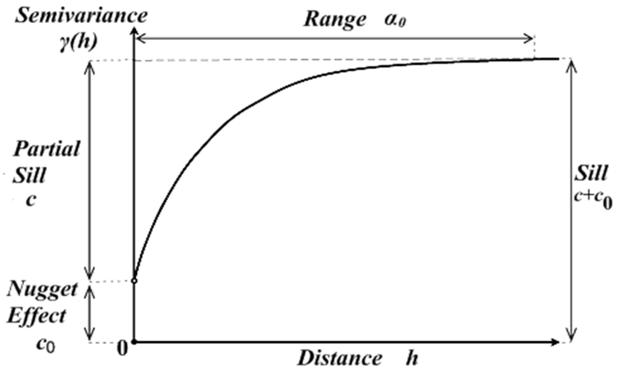
Figure 2.
Components of an ellipse. Source: own elaboration based on [30].
Figure 2.
Components of an ellipse. Source: own elaboration based on [30].
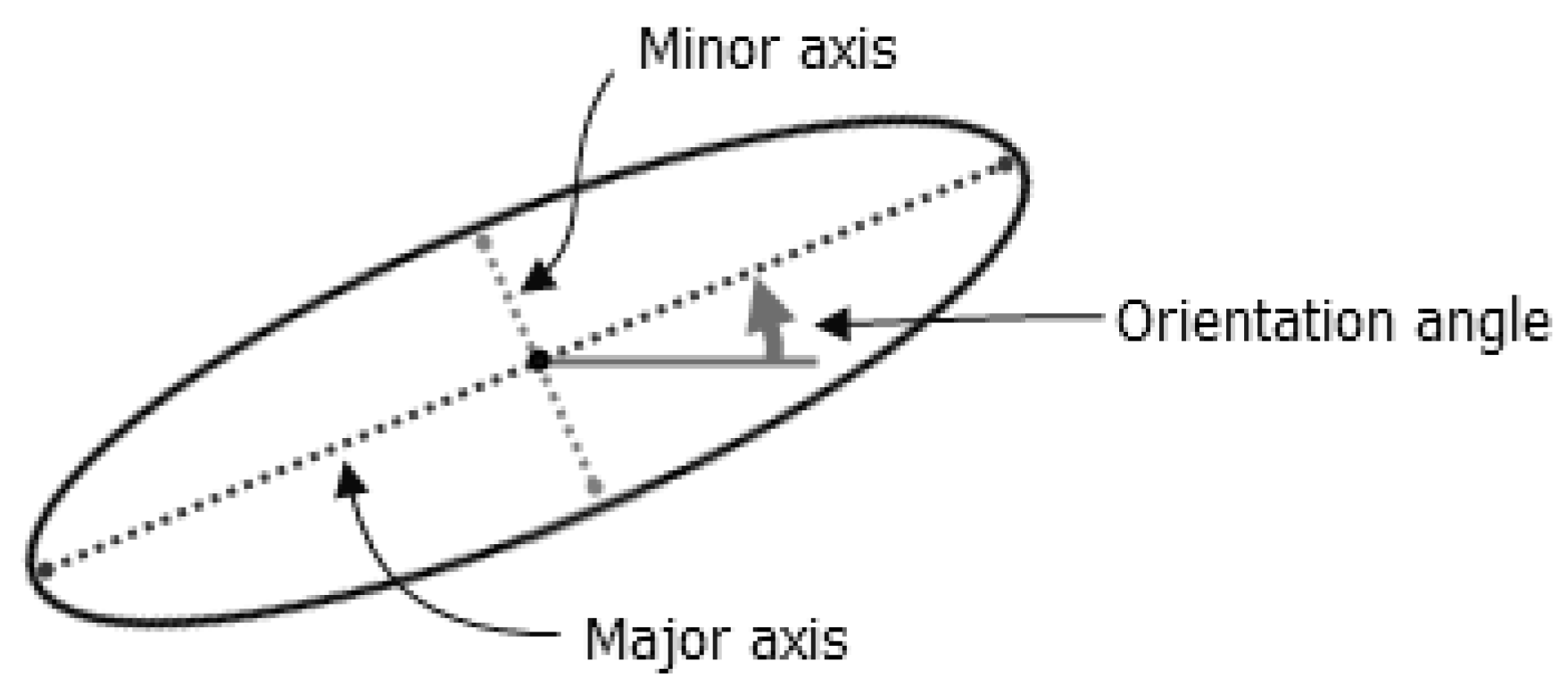
Figure 3.
Semivariogram cloud and models calculated for Wasteav. Note: The data were transformed into a logarithm and detrended; lag size: 14,150.97. Source: own elaboration in ArcMap 10.5.1 based on Table 1.
Figure 3.
Semivariogram cloud and models calculated for Wasteav. Note: The data were transformed into a logarithm and detrended; lag size: 14,150.97. Source: own elaboration in ArcMap 10.5.1 based on Table 1.
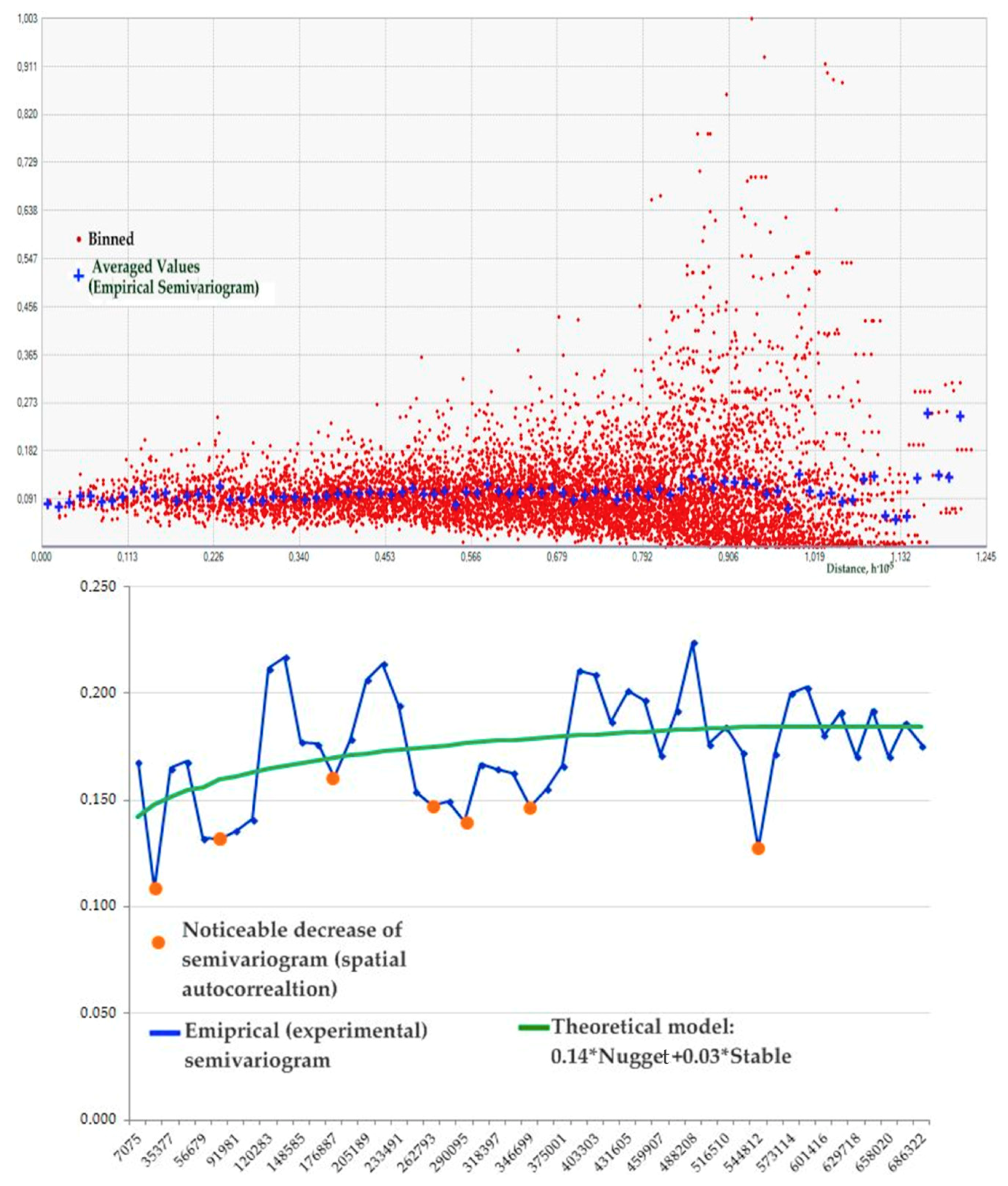
Figure 4.
Semivariogram surface for Wasteav with search direction. Source: own elaboration in ArcMap 10.5.1.
Figure 4.
Semivariogram surface for Wasteav with search direction. Source: own elaboration in ArcMap 10.5.1.
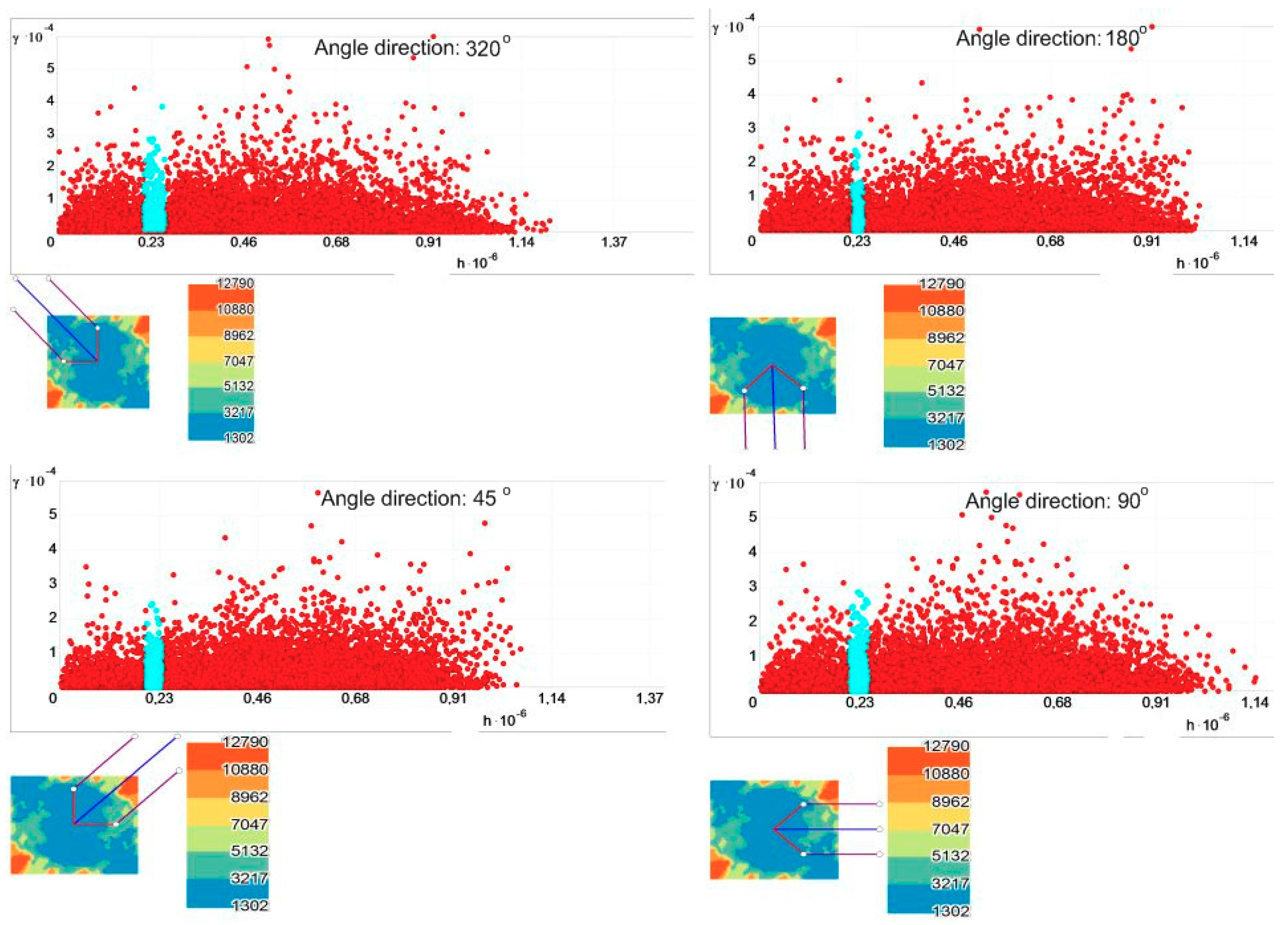
Figure 5.
Spatial trend approximation with the ellipse of two standard deviational distributions and high spatial outliers. Source: own elaboration in ArcMap 10.5.1.
Figure 5.
Spatial trend approximation with the ellipse of two standard deviational distributions and high spatial outliers. Source: own elaboration in ArcMap 10.5.1.
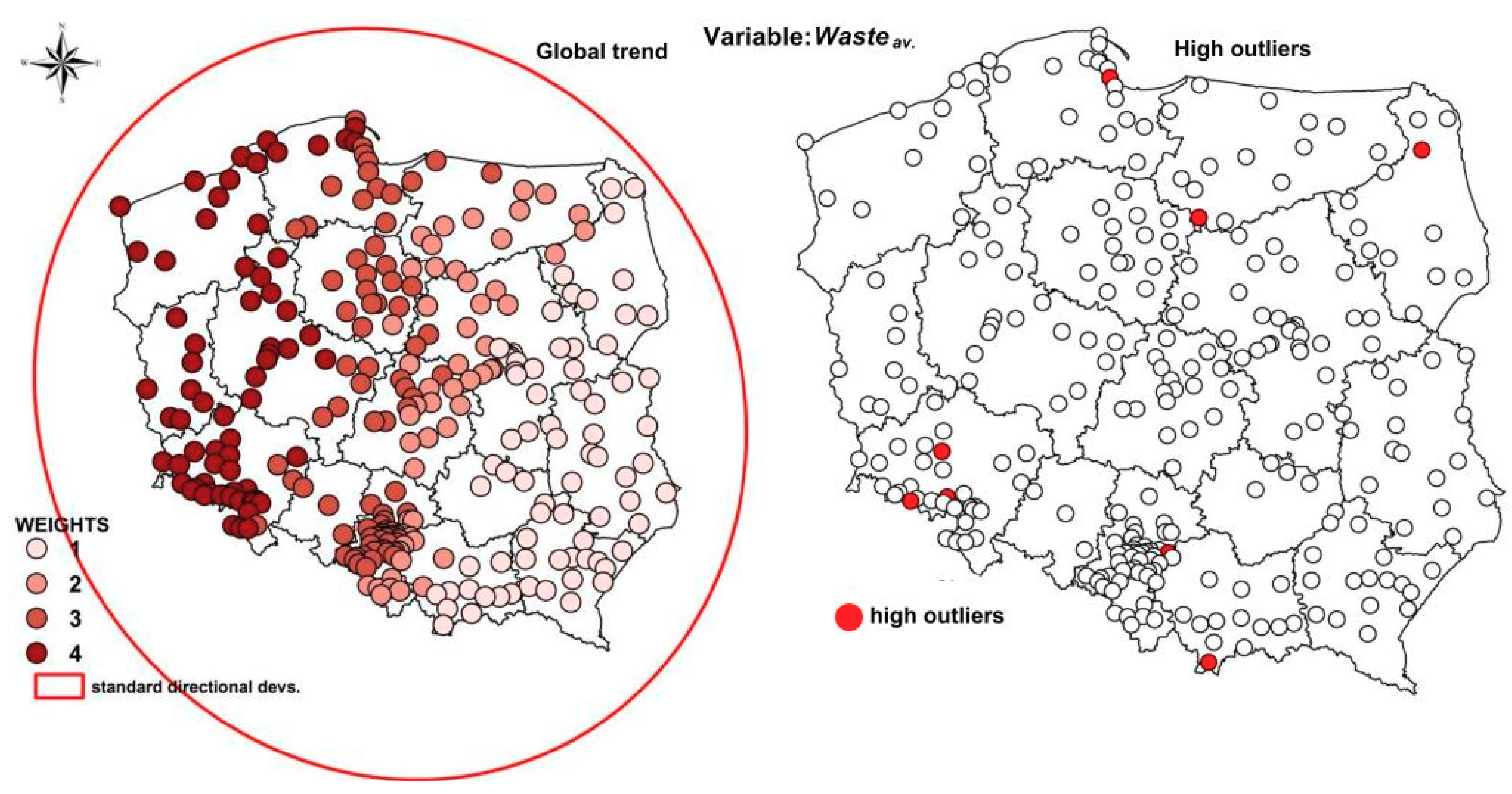
Figure 6.
Local indices of spatial autocorrelation (LISA) results of Wasteav. and W matrices. Note: Statistically significant LISA values vary from 0.01 to 0.05. Source: own elaboration in GeoDa and ArcMap 10.5.1.
Figure 6.
Local indices of spatial autocorrelation (LISA) results of Wasteav. and W matrices. Note: Statistically significant LISA values vary from 0.01 to 0.05. Source: own elaboration in GeoDa and ArcMap 10.5.1.
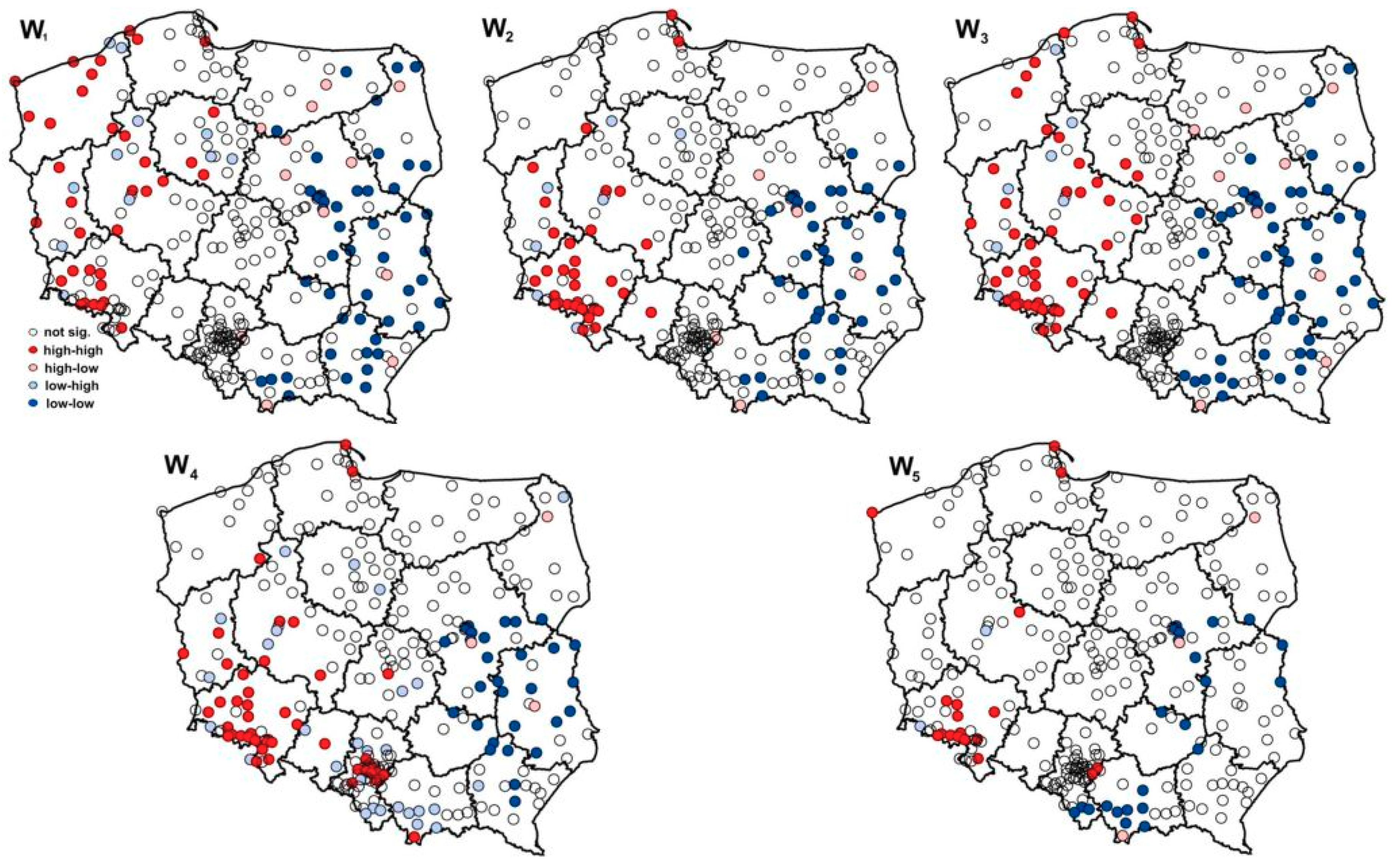
Figure 7.
Mixed municipal waste generated by households, dynamics of the changes of mixed municipal waste generated by households, and economic development (such as the revenues) in selected Polish cities in 2005–2015. Note: Waste—volume of generated municipal waste in kilograms per capita; Revenues—revenues of cities in PLN per capita; dRevenues—dynamics of change of revenues (index); dWaste—dynamics of change of waste (index). Source: own elaboration.

Table 1.
Empirical semivariogram values (averaged) calculated for Wasteav and distance range (in meters).
Table 1.
Empirical semivariogram values (averaged) calculated for Wasteav and distance range (in meters).
| Class | Distance | Semivariogram | Class | Distance | Semivariogram |
|---|---|---|---|---|---|
| Wasteav | Wasteav | ||||
| 1 | 7075 | 0.168 | 21 | 290,095 | 0.140 |
| 2 | 21,226 | 0.109 | 22 | 304,246 | 0.167 |
| 3 | 35,377 | 0.165 | 23 | 318,397 | 0.165 |
| 4 | 49,528 | 0.168 | 24 | 332,548 | 0.163 |
| 5 | 56,831 | 0.132 | 25 | 346,699 | 0.147 |
| 6 | 77,830 | 0.132 | 26 | 360,850 | 0.155 |
| 7 | 91,981 | 0.136 | 27 | 375,001 | 0.166 |
| 8 | 106,132 | 0.141 | 28 | 389,152 | 0.211 |
| 9 | 120,283 | 0.212 | 29 | 403,303 | 0.209 |
| 10 | 134,434 | 0.217 | 30 | 417,454 | 0.187 |
| 11 | 148,585 | 0.177 | 31 | 431,605 | 0.201 |
| 12 | 162,736 | 0.176 | 32 | 445,756 | 0.197 |
| 13 | 176,887 | 0.161 | 33 | 459,907 | 0.171 |
| 14 | 191,038 | 0.179 | 34 | 474,057 | 0.192 |
| 15 | 205,189 | 0.206 | 35 | 488,208 | 0.224 |
| 16 | 219,340 | 0.214 | 36 | 502,359 | 0.176 |
| 17 | 233,491 | 0.194 | 37 | 516,510 | 0.184 |
| 18 | 247,642 | 0.154 | 38 | 530,661 | 0.173 |
| 19 | 262,793 | 0.148 | 39 | 544,812 | 0.127 |
| 20 | 275,944 | 0.149 | 40 | 558,963 | 0.172 |
Note: The values of Wasteav were transformed into a logarithm and detrended (trend of the first order was removed); grey—the lowest values of the semivariogram (i.e., the distances at which the data become the most spatially dependent or autocorrelated); lag size: 14,150.97. The row-standardized weight matrices (distance, directional, and random) for selected years—2005, 2010, and 2015—were also built to examine how results differ considering different spatial matrices (available by email). Source: own elaboration in SAGA and ArcMap 10.5.1.
Table 2.
Values of global Moran’s I statistics for waste using W matrices.
| Moran’s I | Wasteav. | Waste2005 | Waste2010 | Waste2015 |
|---|---|---|---|---|
| Up to 57 km: close (W1) | 0.18 *** | 0.09 *** | 0.17 *** | 0.09 *** |
| Up to 263 km: medium (W2) | 0.16 *** | 0.08 *** | 0.15 *** | 0.08 *** |
| Up to 545 km: far (W3) | 0.07 *** | 0.05 *** | 0.08 *** | 0.04 *** |
| Directional: (W4) | 0.15 *** | 0.20 *** | 0.20 *** | 0.10 *** |
| Random: (W5) | 0.19 *** | 0.15 *** | 0.20 *** | 0.15 *** |
Notes: Significance levels: α = 0.10 *, 0.05 **, 0.01 ***. The Kruskal–Wallis test indicates statistically significant differences (K-W = 12.4 **); Dunn’s multiple comparison test indicates significant differences between results obtained using W3 and W4 as well as W3 and W5. Characteristics of spatial weights matrices; see Table A4 in the Appendix. Source: own elaboration in GeoDa and ArcMap 10.5.1.
Table 3.
Results of the spatial panel estimation.
| Model | Spatial Weight Matrix | α0 | α1 | λ |
|---|---|---|---|---|
| Up to 57 km: close (W1) | 2.25 *** | 0.58 *** | 0.37 *** | |
| Up to 263 km: medium (W2) | 2.25 *** | 0.58 *** | 0.41 *** | |
| Up to 545 km: far (W3) | 2.25 *** | 0.58 *** | 0.44 *** | |
| Directional: (W4) | 2.25 *** | 0.58 *** | 0.10 *** | |
| Random: (W5) | 2.25 *** | 0.57 *** | 0.19 *** |
Note: The values reported in parentheses are p-values. (*), (**), and (***) denote significance at 10%, 5%, and 1%, respectively. Balanced panel: n = 279, T = 11, N = 3069. All variables were expressed in logarithms. Source: own elaboration in R.
Table 4.
Results of the spatial seemingly unrelated regression.
| Model | Spatial Weight Matrix | Year | α0 n | α1 n | λnnn |
|---|---|---|---|---|---|
| W1 | 2005 | 2.31 *** | 0.12 ** | 0.14 | |
| W2 | 2.31 *** | 0.14 ** | 0.16 | ||
| W3 | 2.49 *** | 0.20 ** | −0.02 | ||
| W4 | 2.28 *** | 0.15 ** | 0.18 * | ||
| W5 | 2.52 *** | 0.02 ** | 0.16 ** | ||
| W1 | 2006 | 2.31 *** | −0.03 | 0.23 * | |
| W2 | 2.31 *** | −0.04 | 0.19 | ||
| W3 | 2.35 *** | −0.04 | 0.07 | ||
| W4 | 2.28 *** | −0.05 | 0.18 * | ||
| W5 | 2.35 *** | −0.03 | 0.11 * | ||
| W1 | 2007 | 2.31 *** | 0.008 * | 0.20 * | |
| W2 | 2.31 *** | 0.005 * | 0.16 | ||
| W3 | 2.27 *** | 0.04 * | −0.05 | ||
| W4 | 2.28 *** | 0.01 * | 0.17 * | ||
| W5 | 2.27 *** | 0.04 * | 0.05 | ||
| W1 | 2008 | 2.27 *** | 0.09 * | −0.02 | |
| W2 | 2.27 *** | 0.09 * | 0.003 | ||
| W3 | 2.34 *** | 0.06 * | −0.09 | ||
| W4 | 2.26 *** | 0.10 * | 0.17 ** | ||
| W5 | 2.28 *** | 0.05 * | −0.008 | ||
| W1 | 2009 | 2.29 *** | 0.09 * | 0.32 ** | |
| W2 | 2.29 *** | 0.07 * | 0.30 ** | ||
| W3 | 2.29 *** | 0.002 * | 0.47 ** | ||
| W4 | 2.26 *** | 0.11 * | 0.18 * | ||
| W5 | 2.29 *** | 0.01 * | 0.13 * | ||
| W1 | 2010 | 2.28 *** | −0.02 | 0.28 ** | |
| W2 | 2.28 *** | −0.02 | 0.29 ** | ||
| W3 | 2.32 *** | −0.05 | 0.41 ** | ||
| W4 | 2.24 *** | −0.03 | 0.18 * | ||
| W5 | 2.32 *** | −0.04 | 0.16 ** | ||
| W1 | 2011 | 2.28 *** | −0.004 | 0.21 ** | |
| W2 | 2.28 *** | −0.006 | 0.23 * | ||
| W3 | 2.31 *** | −0.03 | 0.37 ** | ||
| W4 | 2.26 *** | −0.01 | 0.17 * | ||
| W5 | 2.32 *** | −0.001 | 0.17 ** | ||
| W1 | 2012 | 2.27 *** | 0.03 * | 0.21 * | |
| W2 | 2.27 *** | 0.03 * | 0.20 * | ||
| W3 | 2.30 *** | 0.03 * | 0.28 ** | ||
| W4 | 2.23 *** | 0.01 * | 0.18 * | ||
| W5 | 2.29 *** | 0.002 * | 0.11 * | ||
| W1 | 2013 | 2.26 *** | 0.03 * | 0.39 *** | |
| W2 | 2.26 *** | 0.02 * | 0.42 ** | ||
| W3 | 2.37 *** | 0.01 * | 0.41 ** | ||
| W4 | 2.23 *** | 0.01 * | 0.20 * | ||
| W5 | 2.38 *** | 0.01 * | 0.30 *** | ||
| W1 | 2014 | 2.26 *** | −0.01 | 0.40 *** | |
| W2 | 2.26 *** | −0.007 | 0.40 *** | ||
| W3 | 2.32 *** | −0.05 | 0.20 ** | ||
| W4 | 2.24 *** | −0.04 | 0.24 * | ||
| W5 | 2.32 *** | −0.06 | 0.25 *** | ||
| W1 | 2015 | 2.26 *** | 0.04 * | 0.31 ** | |
| W2 | 2.26 *** | 0.04 * | 0.32 ** | ||
| W3 | 2.35 *** | 0.01 * | 0.31 ** | ||
| W4 | 2.24 *** | 0.03 * | 0.20 * | ||
| W5 | 2.35 *** | 0.09 * | 0.23 *** |
Note: The values reported in parentheses are p-values. (*), (**), and (***) denote significance at 10%, 5%, and 1%, respectively; n = 279, T = 11, N = 3069. All variables were expressed in logarithms. Source: own elaboration in R.
© 2018 by the author. Licensee MDPI, Basel, Switzerland. This article is an open access article distributed under the terms and conditions of the Creative Commons Attribution (CC BY) license (http://creativecommons.org/licenses/by/4.0/).
Share and Cite
MDPI and ACS Style
Antczak, E. Building W Matrices Using Selected Geostatistical Tools: Empirical Examination and Application. Stats 2018, 1, 112-133. https://doi.org/10.3390/stats1010009
AMA Style
Antczak E. Building W Matrices Using Selected Geostatistical Tools: Empirical Examination and Application. Stats. 2018; 1(1):112-133. https://doi.org/10.3390/stats1010009
Chicago/Turabian StyleAntczak, Elżbieta. 2018. "Building W Matrices Using Selected Geostatistical Tools: Empirical Examination and Application" Stats 1, no. 1: 112-133. https://doi.org/10.3390/stats1010009