
Global Precedent-Based Extrapolation Estimate of the M8+ Earthquake Hazard (According to USGS Data as of 1 June 2021)


The Zavaritsky Institute of Geology and Geochemistry of the Ural Branch of the RAS, 620016 Ekaterinburg, Russia
*
Author to whom correspondence should be addressed.
GeoHazards 2022, 3(1), 16-53; https://doi.org/10.3390/geohazards3010002
Submission received: 26 November 2021
/
Revised: 14 January 2022
/
Accepted: 18 January 2022
/
Published: 23 January 2022
Abstract
:The paper describes the algorithm and the results of the seismic hazard estimate based on the data of the seismological catalog of the US Geological Survey (USGS). The prediction algorithm is based on the search for clusters of seismic activity in which current activity trends correspond to foreshock sequences recorded before strong earthquakes (precedents) that have already occurred. The time of potential hazard of a similar earthquake is calculated by extrapolating the detected trends to the level of activity that took place at the time of the precedent earthquake. It is shown that the lead time of such a forecast reaches 10–15 years, and its implementation is due to the preservation and stability of the identified trends. The adjustment of the hazard assessment algorithm was carried out in retrospect for seven earthquakes (M8+) that had predictability in foreshock preparation. The evolution of the potential seismic hazard from 1 January 2020 to 1 June 2021 has been traced. It is concluded that precedent-based extrapolation assessments have prospects as a tool designed for the early detection and monitoring of potentially hazardous seismic activity.
1. Introduction
Our research is focused on assessing the predictive capabilities of the equation of Dynamics of Self-Developing Natural Processes (DSDNP equations) and developing algorithms for its practical use. The origin of the first versions of this equation occurred when A. Malyshev (one of the authors of this work) studied plastic deformations that preceded and accompanied the eruptions of Bezymyannyi Volcano in 1981–1984 [1]. These placative deformations were not accompanied by volcanic earthquakes. However, the analysis of changes in the volume of erupted material showed the presence of a direct (the more, the faster) avalanche-like development before the culmination of eruptions and a reverse (the less, the slower) avalanche-like development in the post-climactic eruptive process. Moreover, the absence of signs of an avalanche-like development indicated an upcoming calm (without climactic) eruption. These observations allowed A. Malyshev to successfully predict the directed blast of Bezymyannyi Volcano on 30 June 1985 [1,2,3], as well as a number of eruptions (with or without paroxysm) in 1986 to 1987 [1,3].
The expressions ‘the more, the faster’ and ‘the less, the slower’ are first-order differential equations expressed in words. In these equations, the rate of change in the state of the system depends on its current state. At the same time, the fact of self-development of the system is essential. As a result of the analysis of the patterns of self-development of a wide range of natural processes, it was concluded that, in the case of Self-Developing Systems (SDS), the forces that change their state arise due to their own energy of movement of these systems [1]: Fx = C |Ex − E0|γ = C |mx(x′)2/2 − mx(x′0) 2/2|γ. Here, mx, Fx and Ex are, respectively, the “measure of inertness,” the “force” and the “energy of motion” of the system with respect to parameter x; C is a constant of proportionality; γ is an exponent of nonlinearity and x′ and x′0 are the rates of change of the parameters in the current and stationary states, respectively. This conclusion was transformed into the DSDNP equation [4,5]:
where x is the quantitative parameter of the process, x′ and x″ are the rate and acceleration of changes in this parameter at time t (the first and second derivatives), respectively, k is the proportionality coefficient and exponents λ and α describe the nonlinearity of the process near the stationary state (x′ ≈ x′0) and at a significant distance from it (x′ >> x′0). The above conclusion about the self-development of natural systems corresponds to DSDNP Equation (1) at λ = 2, α = 2γ and k = Cmxγ−1.
x″ = k |(x′)λ − (x′0)λ|α/λ,
Equation (1) is difficult to use in practice. Therefore, in our research, we used a simplified version of the equation as an approximation model:
x″ = k (x′)α.
Equation (2) corresponds to potentially catastrophic processes with a large range of changes in parameter x.
Equation (2) formally corresponds to the equation proposed by B. Voight [6] for describing the dynamics of brittle deformations (disjunctive dislocations) on the eve of the culmination of volcanic eruptions. The Voight equation is used in the Forecasting Failure Method (FFM). However, in earthquake forecasting, Equation (2) was used for the first time in the pioneering work by G. Papadopoulos [7]. The same equation is used in the Accelerated Moment Release (ARM) method using accumulated moment or Benioff strain [8,9,10]. Attempts to use these methods for predictive purposes have not had success. Moreover, both methods have been criticized. In particular, a number of papers [11,12,13] have claimed that the FFM method is biased and inaccurate even for a retrospective analysis. In turn, the statistical insignificance of the ARM method was justified in Reference [14], where it was shown that the ARM practice carries the hazard of identifying patterns that are not real but are created by choosing the free parameters for demonstration of the hypothesized pattern. This hazard is particularly high when the results are unstable.
Serious criticisms have led to a reduction in the number of attempts to use Equation (2) for predictive purposes. Currently, only a few researchers using the ARM method (primarily References [15,16]) are trying to cope with the criticism (‘gravestone’ on this issue) of J. Hardebeck and coauthors [14]. In addition, the Self-Developing Process (SDP) method [17,18] is actively used to study the seismicity of Sakhalin Island and adjacent territories (Russia). The SDP method was developed by I. Tikhonov based on the DSDNP equation for analyzing the flux of seismic events. Nevertheless, all the criticisms expressed in Reference [14] apply to this method as well.
In our opinion, both points of view (supporters of both the FFM and ARM methods and their opponents) have a right to exist. Each researcher can use intuition in his scientific research, but he must (1) consolidate the results obtained in objective and reproducible criteria and (2) confirm the receipt of similar results using these criteria on the maximum possible number of examples (wide test control). An analysis of critical comments on the FFM and ARM methods showed that one of their main problems is the instability of the results obtained. We can confirm the seriousness of this problem due to the experience of our own research. The instability of the results, in our opinion, is largely due to the choice of the optimization criterion: the standard least squares method, commonly used by researchers (in particular, in References [11,12,13]), does not provide the stability of approximation modeling and is therefore ineffective. The Revised-ARM method [15,16] does not solve this problem either. Therefore, the passage of the ARM method through a wide test control seems unlikely. As for the Tikhonov method [17,18], in our opinion, it needs objective criteria for the selection of representative earthquakes and the subsequent receipt of the results in automatic mode.
Our approximation algorithms were configured and successfully tested on synthetic catalogs during the second half of the 1990s. However, subsequent extensive testing on real seismic catalogs showed the instability of the results until the generally accepted optimization criterion for the smallest standard deviations was replaced by optimization for the minimum area deviations in the mid-2000s [5]. Further, the problem with the missing assessment system for the predictability of seismic trends got in the way of our research. This evaluation system was developed by us by the mid-2010s [19]. Optimization by area deviations proved inconvenient for predictive estimates. Therefore, it was replaced by optimization based on bicoordinate (mean geometric) deviations, which also provided the necessary stability to the results obtained. As a result, an algorithm was developed to identify seismic trends and assess their predictability (extrapolability). This algorithm has been extensively and successfully tested on real seismic catalogs when they are fully scanned in automatic mode. The initial version of the algorithm was applied to localized volcanic seismicity [19,20]. Then, this variant was adapted to a 3D space and used in the study of the predictability of seismic trends according to the Kamchatka Regional Catalog (KAGSR) [21], seismic catalogs of the US Geological Survey (USGS) [22,23] and the Japan Meteorological Agency (JMA).
The results of the above works show a good predictability of the seismicity trends, including both trends of increasing activity before strong earthquakes and trends of the attenuation of activity after these earthquakes. However, it should be emphasized here that ‘the predictability of the seismic trend before a strong earthquake’ and ‘the forecast of a strong earthquake’ are not equivalent concepts, even if a strong earthquake fully corresponds to the extrapolation (forecast) part of the trend. Any earthquake that is part of the seismicity trend forms a deviation from the main trend pattern. The prediction of the time and magnitude of these random fluctuations (located in the band of permissible deviations) is difficult even with good predictability of the trend itself.
Thus, the use of Equation (2) in the prediction of strong earthquakes has natural limitations. Nevertheless, the approximation–extrapolation technique developed on the basis of the DSDNP equation, in our opinion, is a good tool for retrospectively studying the patterns of preparation of strong earthquakes and identifying their hazards in real time. When generalizing the previously obtained results on the flux of seismic energy, it was found [24] that the range of values of the parameters α and k in Equation (2), which determined the predictability of strong earthquakes, in the diagram α–lg k (Figure A1) is shifted to the left and below the entire area (including conditionally safe) predictability, i.e., to where the figurative points of the most slowly developing and long-term activation processes are located. This makes it possible to differentiate the trends in the activation of the seismic energy flux by the α and k parameters, on the one hand, into conditionally safe (without precedents of termination by strong earthquakes), and, on the other hand, into potentially hazardous ones that deserve close attention due to the precedents (often repeated) of these trend completions with strong earthquakes. This paper describes an algorithm for estimating the hazard of strong earthquakes and illustrates its use for the flow of seismic energy based on the analysis of data from the USGS catalog as of 1 June 2021.
About terminology. Earthquake sequences are divided by the sign of the coefficient k in the approximation–extrapolation trend: k > 0—activation sequences, k = 0—stationary sequences and k < 0—attenuation sequences. Foreshock sequences are activation sequences that end with strong earthquakes. Foreshocks—all earthquakes of the foreshock sequence preceding a strong earthquake. Aftershock sequences are attenuation sequences that begin after a strong earthquake. Aftershocks—all earthquakes of the aftershock sequence after the main shock. In this paper, only activation sequences and (among them) foreshock sequences are considered. In relation to the time of the mainshock, there are [7,25] close (from several hours to several days), short-term (up to 5 to 6 months) and long-term (several years) foreshocks among the foreshocks. We examine all the listed types of foreshocks without exception.
2. Materials and Methods
2.1. The Model Equation
The solutions of Equation (2) can be expressed in the explicit form:
| k = 0 | x = x1 + x’(t − t1), x′ = const |
| k ≠ 0, α ≠ 1, α ≠ 2 | x = Xa + [k(α − 1)(Ta − t)](α−2)/(α−1)/[k(2 − α)], Ta = t1 + (x′11−α)/[k(α − 1)], Xa = x1 + (x′12−α)/[k(α − 2)] |
| k ≠ 0, α = 1 | x = Xa + (x1 − Xa) exp[k(t − t1)], Xa = x1 − x′1/k |
| k ≠ 0, α = 2 | x = x1 + ln|(Ta − t1)/(Ta − t)|/k, Ta = t1 + 1/(kx′1) |
Thus, the solutions of Equation (2) are either directly a linear dependence (k = 0) or are reduced to linear dependences by taking the logarithm of the differences between the parameter values and/or time and the respective asymptotes:
| k ≠ 0, α ≠ 1, α ≠ 2 | ln|x − Xa| = c1ln|t − Ta| + c0, c1 = (α − 2)/(α − 1), c0 = ln|k(α − 1)|(α − 2)/(α − 1) − ln|k(α − 2)| |
| k ≠ 0, α = 1 | ln|x − Xa| = c1t + c0, c1 = k, c0 = ln|x1 − Xa| − k × t1 |
| k ≠ 0, α = 2 | x = c1ln|Ta − t| + c0, c1 = −1/k, c0 = x1 + ln|Ta − t1|/k |
2.2. The Optimization and Its Criteria
The linearity of solutions of Equation (2) in ordinary or logarithmic coordinates simplifies optimization (finding the best match to the factual data). Direct optimization by five values (α, k, x1, x′1 and t1) is complex and requires large computing resources. However, when using solutions from Equation (2) in linear form (conventional or logarithmic), optimization is reduced to the analysis and comparison of several variants of linear regression. In some cases, optimization may also be required with respect to one or two additional parameters: Ta and/or Xa. The optimal values (α, k, x1, x′1 and t1) for each variant are easily determined analytically from linearity constants (c0, c1) and asymptotes (Ta and/or Xa). This greatly simplifies the optimization procedure and reduces the requirements for computing resources.
For the stability of the results, it is of great importance to choose an optimization criterion—a quantitative characteristic of the correspondence between the factual data and their approximation model. Therefore, to solve the problems that arise (see their detailed description in Reference [22]), all variants of linear regression are compared in ordinary (nonlogarithmic) coordinates. The bicoordinate rms deviation Δxt = {Σ(ΔxiΔti)/[n(xc − xs)(tc − ts)]}0.5 is used as an optimization criterion to ensure the stability of the results. Here, (xc − xs) and (tc − ts) are the ranges of variations of the factual data for optimization (these ranges normalize the coordinates to a range from 0 to 1), and Δxi and Δti are the deviations of each point of the factual data from the calculated curve along the abscissa and ordinate axes, respectively. In a geometric sense, the bicoordinate deviation corresponds to the side of a square equal in area to a rectangle with sides Δxi and Δti, i.e., the bicoordinate deviation is the geometric mean of these deviations. The bicoordinate root mean square deviation is not the only possible criterion for the stability of the optimization results (optimization by area deviations has been successfully applied before), and moreover, it cannot be argued that this criterion is the best. However, it allows you to get stable results and is adequate for the available computing resources. For greater sensitivity, optimization is performed according to the maximum of the regularity coefficient (the inverse value for bicoordinate deviation): Kreg = 1/Δxt.
2.3. The Processing of Seismic Catalogs
A spatial analysis of seismic data was carried out by spherical hypocentral samples with radii of 7.5, 15, 30, 60, 150 and 300 km. For each radius, the sample centers formed a fixed grid over the entire surface of the Earth and in subsurface spaces up to depths of 1000 km. Within this grid, the sample centers are distributed by latitude, longitude and depth, with an offset step that is 1.5 times smaller than the sample radii (i.e., 5, 10, 20, 40, 100 and 200 km, respectively), which provides spatial overlap of the samples. Catalog processing is executed automatically for each radius. Each event in the analyzed catalog is consistently treated as a ‘current’ event (earthquake). The moment of time of this event is taken as the ‘present’. The time preceding this event is considered the ‘past’, and the subsequent time is considered the ‘future’. To analyze the seismicity preceding and following the ‘current’ event, a spherical sample with the center closest to the hypocenter of the ‘current’ earthquake is used. Within this sample, an array of data of the studied flow parameter is formed (in our case, the flux of seismic energy, i.e., the total energy of earthquakes).
The main trends of the ‘current’ seismicity are revealed by test approximations in order to search the factual data for those intervals that demonstrate the best characteristics during optimization. The first test approximation is performed based on the factual data presented by the ‘current’ earthquake and the 6 preceding ones. In subsequent test approximations, the nearest event from the ‘past’ is added to the approximated factual data until the first event in the sample is included in their number. All approximations with Kreg < 10 are ignored. From all the test approximations, the three best variants are selected: the first one is based on the maximum Kreg, and the rest are based on the nearest and main maxima of the Kreg/Klin ratio. The first variant is always determined, the rest depending on the presence and combination of current nonlinear trends. Nonlinearity variants allow you to track new development trends that begin (and, therefore, are still poorly expressed) against the background of the main trends.
2.4. The Estimation of Extrapolation Predictability
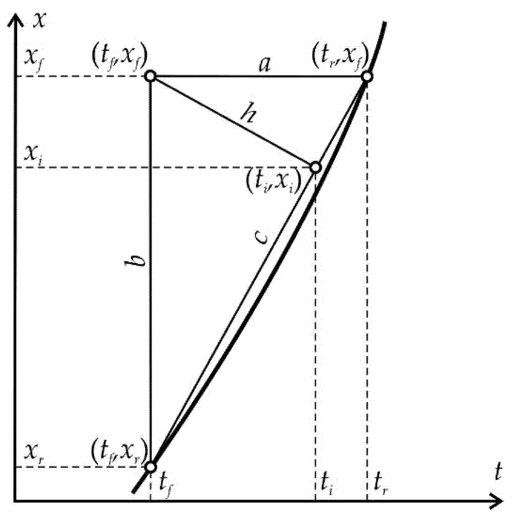
The term ‘trend predictability’ is defined here as finding the factual data of the ‘future’ in the band of acceptable errors relative to the calculated curve in its extrapolation part. To estimate the trend predictability, the rms deviation σ of the factual points (tf,xf) from the calculated curve along the one normal to it is used. It is calculated on the approximation section of the trend in coordinates normalized to a range from 0 to 1 from the first (ts,xs) to the last point (tc,xc):
σ = {Σ[(((xr − xf)/(xc − xs)) × ((tr − tf)/(tc − ts)))2/(((xr − xf)/(xc − xs))2 + ((tr − tf)/(tc − ts))2)]/n}0.5.
Equation (3) is obtained on the basis of elementary geometric constructions (Figure 1), in which the shortest distance from the factual point (tf,xf) to the calculated curve is estimated in the first approximation as the height h of a right triangle (tr,xf)–(tf,xf)–(tf,xr) lowered by the hypotenuse (tr,xf)–(tf,xr) from the opposite vertex, which is the factual point (tf,xf): h = ab/c. As a result, Equation (3) is an expression for the root mean square value of these distances.
Further, the approximation is extrapolated into the ‘future’ as long as the distance of each subsequent (predicted) factual point (tp,xp) to the calculated point is in the band of permissible errors ± 3σ, i.e., the ratio is fulfilled:
[(((xr − xp)/(xp − xs)) × ((tr − tp)/(tp − ts)))2/(((xr − xp)/(xp − xs))2 + ((tr − tp)/(tp − ts))2)]0.5 ≤ 3σ.
The width of the error band here is determined from the statistical rule ‘3 sigma’, according to which, 99.73% of the results fall into such an error band in the case of a normal distribution. Since the ratio (4) uses normalization for the range from 0 to 1 from the first (ts,xs) point to the point being tested (tp,xp), then the average deviation is pre-recalculated to the same normalization range; that is, σ is pre-recalculated on the approximation section of the trend according to Equation (3) with the replacement of tc and xc by tp and xp.
2.5. Quantitative Estimates in Prediction Precedents for Strong Earthquakes
The relative accuracy of the precedent predictions is estimated by the formula:
Δ = (tsh_f − tc)/σt.
Further, the following classification of the accuracy of the retrospective predictions is used in the work: quantitative estimations at Δ ≥ 5 (relative error <20%), semi-quantitative estimations at 2 ≤ Δ < 5 (relative error 20–50%) and qualitative estimations at Δ < 2 (relative error > 50%). Here, the relative error is the inverse of the relative accuracy.
The predicted nonlinearity of Lpn is calculated by the formula:
Lpn = (Δx − Δt)/(Δx + Δt), where Δx = (xsh_f − xs)/(xc − xs) − 1, Δt = (tsh_f − ts)/(tc − ts) − 1.
Factual values (xsh_f, tsh_f) are used in retrospective estimates. When predicting by precedent, instead of them, the calculated values (xsh_i, tsh_i) for a strong earthquake are used in the Equation (6).
In essence, the predictive nonlinearity of Lpn corresponds to the sign of the coefficient k in the DSDNP equation, but not in the integer, except in real terms. For extremely nonlinear activation sequences, parameter predictability dominates over time predictability, so the Lpn value is close to 1. As the ratio in the predictability of the trend in terms of parameter and time is leveled, the Lpn value decreases, reaching 0 for sequences close to stationary development. A further shift of the ratios in trend predictability leads to an increasing increase in time predictability compared to parameter predictability, which corresponds to attenuation sequences. Lpn values tend to be −1 for extremely nonlinear attenuation sequences, in which the time predictability significantly exceeds the parameter predictability. Thus, for the activation sequences considered by us (foreshock sequences in case of the completion of activation by a strong earthquake), the Lpn value varies from 0 to 1. As will be shown below on the example of retro-forecasts, the predictive nonlinearity of the Lpn determines the asymmetry of the band of permissible deviations and thereby reflects the stochasticity/determinism of the position (fluctuations) of the main thrust of the predicted trend.
The approximation–extrapolation coefficient A shows how many times the general trend of activation exceeds the approximation part included in it. This coefficient is calculated in the coordinates of the full trend, normalized to a range from 0 to 1 and is used to estimate the limit of possible extrapolations. In general, the value of A can be determined by the ratio of the lengths of the corresponding sections of the calculated curve; however, in the case of step cumulative characteristics of the seismic flow (energy, Benioff strain or the number of events), the formula is simpler and quite effective:
A = 2/[(xc − xs)/(xsh_f − xs) + (tc − ts)/(tsh_f − ts)].
When predicting by a precedent, instead of the factual values (xsh_f,tsh_f) in Equation (7), calculated values (xsh_i,tsh_i) for a strong earthquake are also used.
2.6. The Real-Time Predictive Estimation Algorithm
The use of the precedents from retro-forecast data is based on the possibility of linking the time tsh_f of the main earthquake to the rate x′sh of change of the parameter at the point of the extrapolation curve closest to the main earthquake. In retrospective studies, this point is determined in parameter–time coordinates, normalized to a range from 0 to 1 according to the factual values from point (ts,xs) to point (tsh_f,xsh_f). If the factual point of a strong earthquake is located within the region of existence of the extrapolation curve (tsh_f < Ta at α > 1 and xsh_f < Xa at α > 2), then the distances to the extrapolation curve from the factual point of a strong earthquake are determined by the abscissa (a) and ordinate (b): a = |tsh_f − t(xsh_f)|, b = |xsh_f − x(tsh_f)|. Geometrically, these distances correspond to the cathetus of a right triangle with a vertex at the point (tsh_f,xsh_f) (see Figure 1, assuming that point (tf,xf) is point (tsh_f,xsh_f) and point (ti,xi) is point (tsh_i,xsh_i)). Then, the position of point (tsh_i,xsh_i) is approximately defined as the intersection of the hypotenuse perpendicular to it from the vertex of the right angle. Based on the proportions existing in a right triangle, we determined the coordinate values for this point: tsh_i = tsh_f + (t(xsh_f) − tsh_f)/(a + b) and xsh_i = xsh_f + (x(tsh_f) − xsh_f)/(a + b). Using these coordinates, the rate x′sh is calculated: x′sh = [k(α − 1)(Ta − tsh_i)]1/(1−α) at α ≥ 1.5 or x′sh = [k(2 − α)(xsh_i − Xa)]1/(2−α) at α < 1.5.
If one of the coordinates of the factual point of a strong earthquake goes beyond the area of existence of the extrapolation curve, then the nearest point of the calculated curve is determined by the second coordinate (abscissa or ordinate, respectively): xsh_i = x(tsh_f) and tsh_i = tsh_f or tsh_i = t(xsh_f) and xsh_i = xsh_f. After that, the rate x′sh is calculated according to the above formulas. If both coordinates go beyond the limits of the existence of the extrapolation curve (tsh_f ≥ Ta and xsh_f ≥ Xa at α > 2), the asymptotic point (Ta,Xa) turns out to be the closest to the earthquake; therefore, an extremely large value is conditionally assumed as the rate x′sh.
The regularities of the precedent foreshock preparation of strong (M7+) earthquakes allow identifying similar trends in the seismic activity increase. The prediction estimates of these trend hazards assume the use of the data of precedent retrospective predictions and are based on the possibility of binding the time of the main earthquake to the rate of change in the x′sh parameter at the point of the extrapolation curve closest to the main earthquake. For this purpose, a database of precedent retrospective predictions is created. This database includes information about the hypocentric radius of the sample, α, k and x′sh, as well as information about this strong precedent earthquake (magnitude, time and place).
The essence of the precedent–extrapolation assessment of a seismic hazard is to identify potentially hazardous spatial zones where there is such an increase in seismic activity that has historical precedents of ending with a strong earthquake. The quantitative aspect of the forecast corresponds to the calculation of the possible time of a similar earthquake based on the database of its previous forecasts. For the activity in each spatial zone, analogs are possible in the preparation of several strong earthquake precedents. In this case, calculations of the possible time of a similar earthquake in the considered spatial region are performed for each of the precedents.
The prediction extrapolations algorithm provides for the following operations:
- Search in the catalog for unfinished (not come out of the band of admissible errors at the time of the catalog end) prediction definitions, in which a tendency towards an increase in seismic activity is found.
- Comparison of the type of an activity increase with the database of precedent retrospective predictions alongside the sample radius, exponent α (with an accuracy of 0.01) and coefficient k (when comparing lg k with an accuracy of 0.1). All cases of an activity increase that have no analogs in the database of precedent retrospective predictions are ignored.
- For each precedent retrospective prediction based on the rate of change in the x′sh parameter, the time tsh and the value of the xsh parameter are calculated, at which, for a given type of an activity increase, its level will correspond to the level of the precedent shock:tsh_i = Ta − x′sh1−α/[k(1 − α)] when α ≠ 1 or tsh_i = t1 + ln(x′sh/x′1)/k when α = 1,xsh_i = Xa − x′sh2−α/[k(2 − α)] when α ≠ 2 or xsh_i = x1 + ln(x′sh/x′1)/k when α = 2.Then, the values of Lpn, A and σt are estimated. The definitions, for which the approximation and extrapolation ratio A exceed the maximum value of Amax for retro-forecast precedents, are considered as having no precedents.
- The revealed precedent retrospective predictions are grouped by the main shock. For each group, the calculated average time of the strong earthquake and its standard deviation σsh, as well as the average values of Lpn, A and σt, are determined.
2.7. Initial Data
As the initial data for a precedent-based extrapolation estimate of the M8+ earthquake hazard, this work uses the worldwide United States Geological Survey (USGS) earthquake catalog [26], which includes data from 1900 to the end of May 2021. By this time, the catalog contains data on 3,889,120 earthquakes with a magnitude M = −1.0 … +9.5 at its modal value 1.2. The results of processing the Japan Meteorological Agency (JMA, 1919–present) earthquake catalog [27] and the Earthquakes Catalogue for Kamchatka and the Commander Islands (ECKCI, 1962–present) [28] were also used to analyze the foreshock predictability and form a database of precedent retro-forecasts. By the end of August 2018, the JMA catalog contained data on 3,498,071 earthquakes with a magnitude M = −1.6 … + 9.0 at its modal value 0.6. By the end of March 2021, the ECKCI catalog contained data on 428,225 earthquakes with a magnitude M = –2.7 … + 8.1 at its modal value 0.5. The seismic energy flux E is considered as the x parameter, i.e., a cumulative amount of earthquakes energy. In this case, the energy of a single earthquake is estimated according to the existing relationship between its magnitude M and the energy class K [29]: K = lg E = 1.5 M + 4.8. The relationship between M and energy E is valid for E in Joules. When processing catalogs, all earthquakes are used, for which there are energy characteristics (M or K), regardless of their magnitude. Our research does not require the completeness of seismic catalogs and does not depend on it. We study the flow of seismic energy as it is (where it is recorded and how it is recorded). This is of great importance for this work, since the USGS world catalog is made up of many regional catalogs and, therefore, is extremely heterogeneous in completeness both in space and in time.
3. Results
3.1. Analysis of Retro-Precedents of Foreshock Forecasting
As a result of processing the ECKCI, JMA and USGS data, it was found that the predicted activation of the seismic energy flow precedes 721 out of 2082 earthquakes with M ≥ 7 (8 out of 17 ECKCI, 123 out of 676 JMA and 590 out of 1389 USGS). It was found that 116,700 (1553 ECKCI, 87,474 JMA and 27,673 USGS) precedents of these earthquakes fall into the band of acceptable errors when retrospectively extrapolating foreshock trends into the ‘future’. In particular, one of the most powerful earthquakes of this number—the Tohoku earthquake on 11 March 2011 (M = 9.0 JMA and M = 9.1 USGS)—had 189 (150 JMA and 39 USGS) precedents of falling into the band of retro-forecast extrapolations. A significant number of strong earthquakes that do not have a predictable preparation, in our opinion, is due to the absence or insufficient level of registration of seismicity in the period preceding these earthquakes.
3.1.1. The Relationship between the Predicted Nonlinearity of the Seismic Energy Flow and the Determinism of Strong Earthquakes
Examples of retrospective prediction extrapolations with a sufficiently high relative accuracy Δ and significant differences in predicted nonlinearity Lpn are shown in Figure A2. Table A1 contains data on the main shock, sample and some characteristics of the foreshock trend corresponding to these examples. It can be seen in Figure A2 that, for a low predicted nonlinearity Lpn (graph in Figure A2a), the position of the strong earthquake step in the energy flux is weakly determined by the band of admissible deviations. A strong earthquake in this band could have occurred both much earlier and much later than its factual time, i.e., the stochasticity of a strong shock time increases with decreasing the predicted nonlinearity. The latter is typical for the sequences of activation close to stationary development. On the contrary, with an increase in the predicted nonlinearity (graphs in Figure A2b–f), the asymmetry of the band of admissible deviations by the parameter and time increases. As a result, the step of a strong earthquake, requiring a large admissible deviation by the parameter, is more and more rigidly determined by a reduction of the time interval, in which a strong shock can occur. This variability of stochasticity/determinacy of the process, depending on the level of predicted nonlinearity Lpn, has to be taken into account in predictive extrapolation calculations of the time of strong earthquakes.
3.1.2. Statistics of Lead Time, Relative Accuracy and Approximation-Extrapolation Ratio in Retro-Forecasts of Strong Earthquakes
In the distribution of retro-forecast precedents according to their lead time (Table A2), first of all, the high proportion of retro-forecasts separated from the main shock by large time intervals attracts attention. Almost 20% of predictions have a lead time of 3 to 10–15 years or more (f.e., graphs in Figure A2b,d). Almost 43% of retro-forecasts have a lead time of 3 months to 3 years (f.e., graphs in Figure A2c,e).
Retro-forecasts of strong earthquakes have, on average, a semi-quantitative level of relative accuracy (Δaverage = 3.26, Table A3). However, a high lead time in the range of 3 years or more leads to an increase in the average relative accuracy of forecasting to a quantitative level (Δaverage = 5.69 for (tsh_f − tc) > 1000 days; see Table A3). There is also a general tendency to further increase the average relative accuracy for the most deterministic earthquakes (with the highest level of predictive nonlinearity, Lpn).
With a decrease in the lead time, the average relative accuracy of retro-forecasts decreases until the transition to a qualitative level at (tsh_f − tc) < 10 days. Nevertheless, against the general background of this decline, retro-forecasts with a quantitative level of accuracy are noted at all time ranges. Thus, the distribution of retro-forecast definitions by their lead time and accuracy indicates the possibility of, at least, medium long-term quantitative predictions of strong earthquakes with the prospect of quantitative forecasting at all ranges of lead time.
When switching to predictive extrapolations in real time, it is necessary to take into account that almost all trends in the activation of the energy flow with an unlimited extrapolation can reach a level sufficient for a strong earthquake. However, the real possibilities of predictive extrapolation are limited. As can be seen in Table A4, the approximation–extrapolation ratio in foreshock retro-forecasts does not exceed the value of Amax = 2.50. It follows from this that, for sequences with weakly expressed predictive nonlinearity (and, accordingly, approximately proportional increments in the predictive part of the parameter and time), the time extrapolation cannot exceed the duration of the approximation component of the trend by more than 1.5 times. For extremely nonlinear sequences, in which almost all the increments of the parameter fall on the forecast part of the trend, the extrapolation possibilities are reduced in time and are limited to 20% of the duration of the approximation component of the foreshock trend. In addition, the data in Table A4 indicate that both the maximum and average values of the approximation–extrapolation ratio A tend to increase with the increasing lead time and predictive nonlinearity of retro-forecasts.
3.2. Precedent-Based Extrapolation Estimation of Seismic Hazard in Retrospect
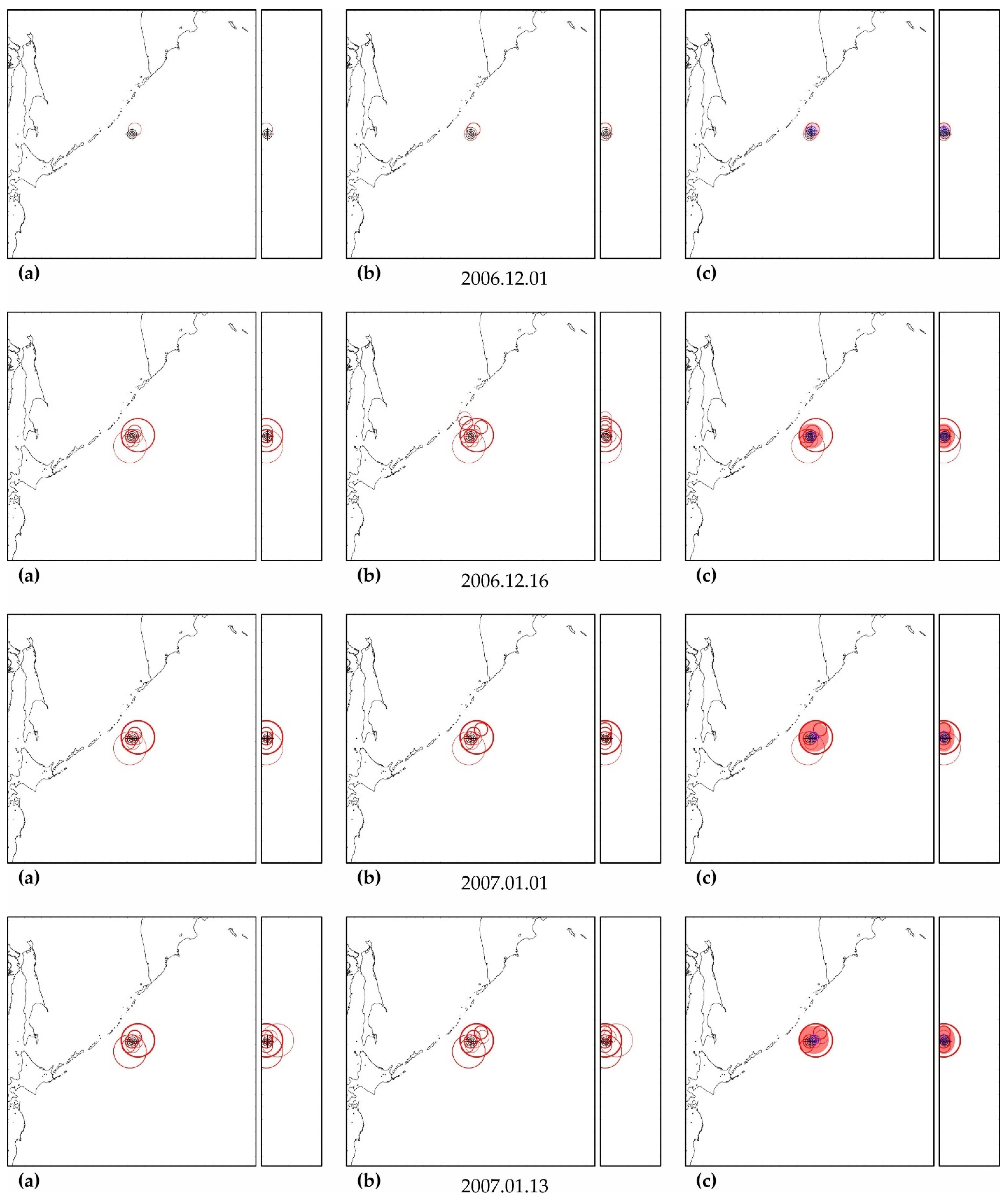
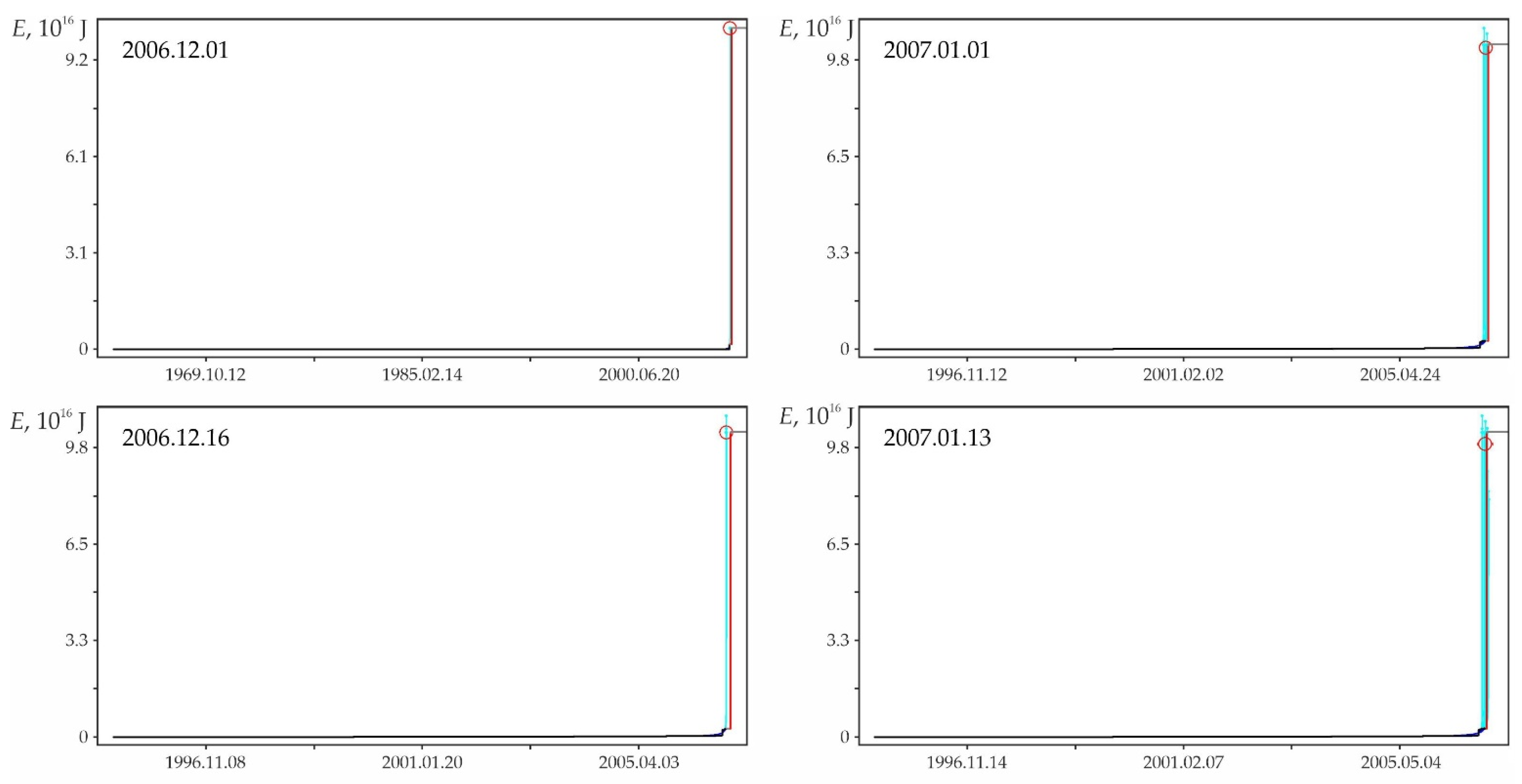
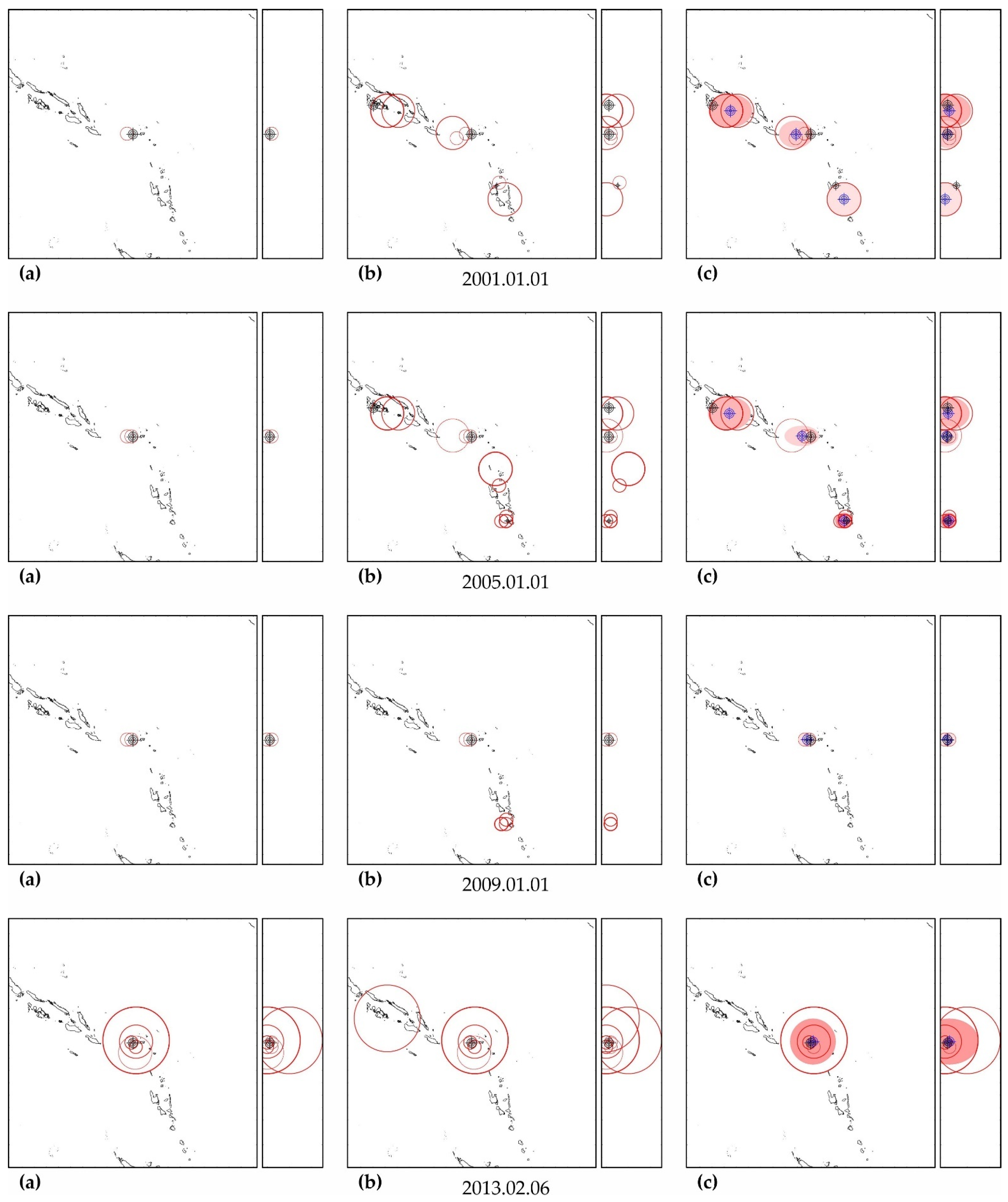
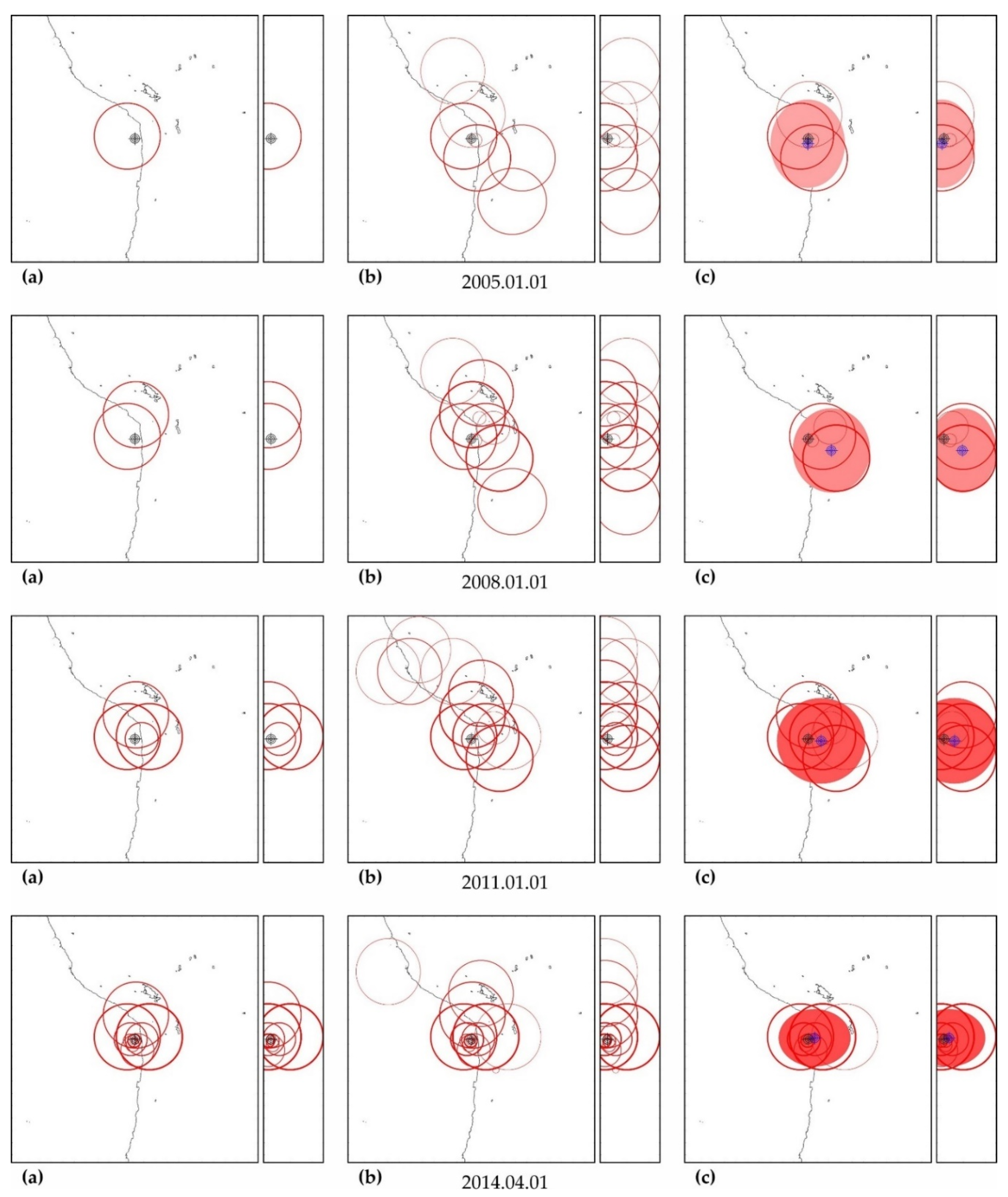
When assessing the seismic hazard, data from M8+ earthquake retro-forecasts are used (Table 1), having a sufficiently high level of predictive nonlinearity Lpn ≥ 0.9. Seven strong earthquakes used as precedents according to the USGS catalog have 597 precedent forecasts. This corresponds to 20% of the number of precedent earthquakes and 79.5% of the number of precedent forecasts based on the results of processing the USGS catalog. These earthquakes are used to retrospectively adjust the algorithm of precedent-based extrapolation estimations (see Appendix B): M8.0 earthquake on 16 November 2000 (−3.980° latitude, 152.169° longitude, 33-km depth)—30 precedent forecasts; M8.1 earthquake on 13 January 2007 (46.243°, 154.524°, 10)—52 precedent forecasts; M8.4 earthquake on 12 September 2007 (−4.438°, 101.367°, 34)—178 precedent forecasts; M9.1 earthquake on 11 March 2011 (38.297°, 142.373°, 29)—39 precedent forecasts; M8.0 earthquake on 6 February 2013 (−10.799°, 165.114°, 24)—34 precedent forecasts; M8.2 earthquake on 1 April 2014 (−19.610°, −70.769°, 25)—244 precedent forecasts and M8.0 earthquake on 26 May 2019 (−5.812°, −75.270°, 122)—20 precedent forecasts.
As can be seen in Figure A3, Figure A5, Figure A7, Figure A9, Figure A11, Figure A13 and Figure A15, in columns (a), the predictability of each of these earthquakes is noted simultaneously in several zones, forming a spatial cluster. However, similar activity is observed not only in the earthquake preparation zone, where it is maximal, but also outside it (see column (b) in the figures listed above). Therefore, the cluster of activity is identified according to the zone with the largest number of unfinished potentially hazardous extrapolations with similar precedent activity. Together with the zone of maximum activity, all the closest zones with similar activity that intersect with the maximum zone are combined into a cluster. The intersection of two cluster zones is understood here as finding the hypocenters of these zones from each other at a distance less than the radius of the biggest zone.
The cluster center (and hypocenter of a possible earthquake) is calculated as the weighted average (by the number of potentially hazardous extrapolations) center of all cluster zones. Similarly, the boundaries of the cluster ellipsoid in latitude, longitude and depth are calculated based on the hypocentral radii of the zones included in the cluster. The results of the allocation of cluster zones and the determination of the cluster ellipsoid and the estimated position of the hypocenter of a possible earthquake are shown in column (c) in the figures listed above. The errors in determining the hypocenter Derr (the distance between their factual and calculated positions) are given in Table A5, Table A6, Table A7, Table A8, Table A9, Table A10 and Table A11.
In all cases, the actual hypocenter falls into the calculated ellipsoid of cluster activity. This is the expected result corresponding to the successful testing of cluster algorithms for earthquakes on the example of their own precedent forecasts. However, in a number of cases, when testing the predictability according to the data of one earthquake, similar foreshock preparation and cluster predictability for other earthquakes were found. In particular, when testing predictability on the example of the earthquake of 16 November 2000 (M8.0), a cluster of predictability with a similar preparation for the earthquake of 1 April 2007 (M8.1) was additionally detected in all hazard estimates (see Figure A3); when testing on the example of the earthquake of 6 February 2013 (M8.0), the predictability clusters of three more earthquakes (9 January 2001, M7.1; April 1, 2007, M8.1 and 10 August 2010, M7.3) were also additionally detected (see Figure A11). These facts can be considered as an additional justification for the possibility of applying precedent-based extrapolation estimates in real-time.
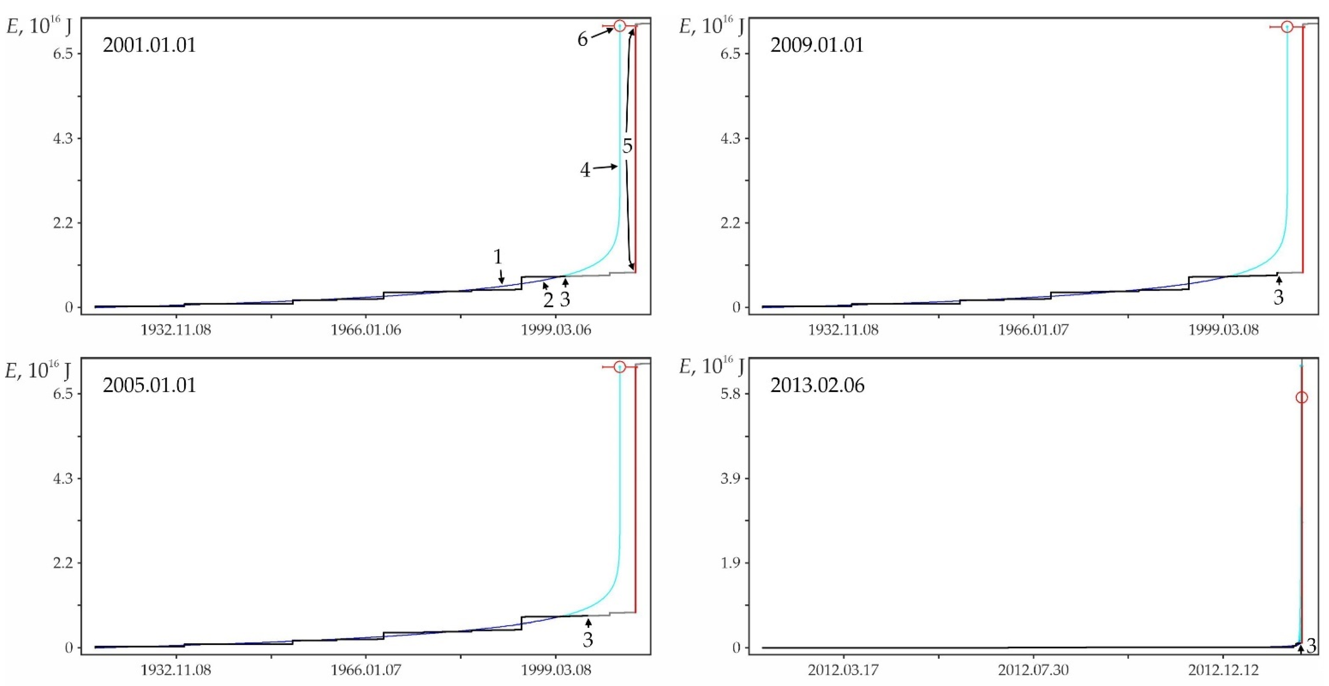
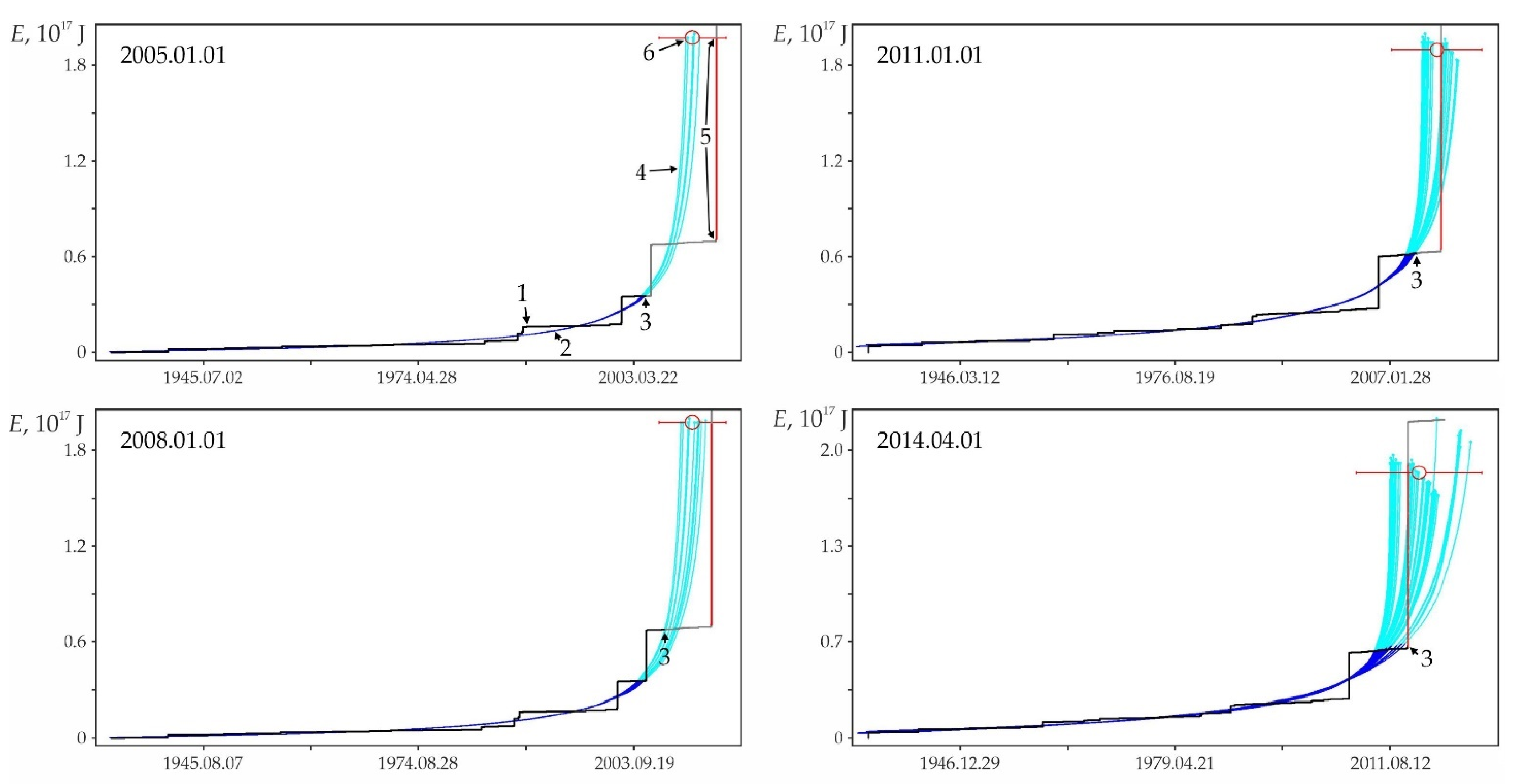
In a number of cases, cluster definitions of the time of a possible shock demonstrate the quantitative accuracy of the forecast: the relative error of the estimated time of the earthquake of 11 March 2011 (M9.1) is 2.58% in the estimate of 1 January 2009 (see Table A8); for the earthquake of 6 February 2013 (M8.0)—2–4% in the estimate of 2007–2010 and 2012 (see Table A9), etc. However, often, these accurate forecasts are side by side or interspersed with semi-quantitative and qualitative estimates. Moreover, all forecast retro-forecast estimates for the time of the earthquake of 13 January 2007 (M8.1) are in the ‘past’, although the earthquake itself occurs in the ‘future’ (see Table A6). This is the correct location of the estimated time in the band of permissible deviations. Since the relative accuracy of the precedent calculations is unstable, and its real value can be estimated only in the future based on the actual result so far, we are forced to focus on the worst level of accuracy, i.e., on the qualitative relative accuracy of precedent estimates of the time of a possible earthquake. Therefore, we can consider the fact of the formation of a cluster of potentially hazardous activity only as a precursor of a possible strong earthquake. Accordingly, all retro-forecasts of the time of a possible strong earthquake with a quantitative level of accuracy at this stage of research can be considered only as random coincidences.
3.3. Precedent-Based Extrapolation Estimation of Seismic Hazard in Real-Time
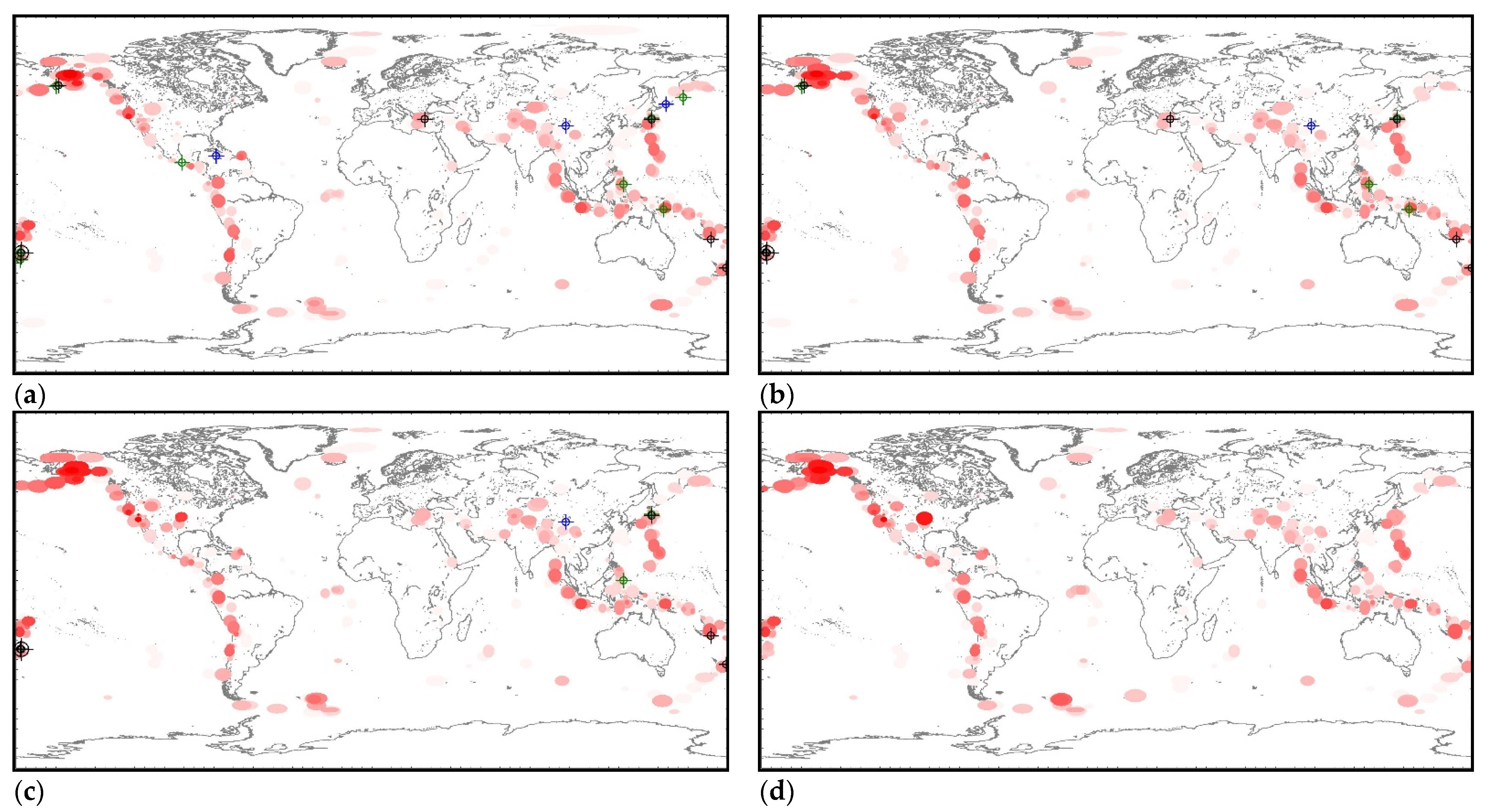
We made four global hazard estimates based on the USGS catalog (Figure A17): as of 1 January 2020, as of 1 July 2020, as of 1 January 2021 and as of 1 June 2021. The first three were intended for control testing and tracking changes of global hazards, and the last one was a real-time estimate at the end of the processed catalog. The test period covered 1 year and 5 months. During this period, 17 M7+ earthquakes occurred in the world, including one M8+ earthquake. Of this number, seven (41%) M7+ earthquakes (including a single M8+ earthquake) occurred in the identified clusters of hazardous activity and within the error range of the predicted trends (full predictability, Table A12; see also the black circles with a crosshair in Figure A17). Another seven (41%) M7+ earthquakes have partial predictability. They occurred in the identified clusters of activity (see the green circles in Figure A17) but go beyond the permissible errors of predictive extrapolations: M7.5 earthquake on 25 March 2020 (48.964°, 157.696°, 57.8); M7.4 earthquake on 18 June 2020 (−33.293°, −177.857°, 10.0); M7.4 earthquake on 23 June 2020 (15.886°, −96.008°, 20.0); M7.0 earthquake on 17 July 2020 (−7.836°, 147.770°, 73.0); M7.6 earthquake on 19 October 2020 (54.602°, −159.626°, 28.4); M7.0 earthquake on 21 January 2021 (4.993°, 127.515°, 80.0); M7.0 earthquake on 20 March, 2021 (38.452°, 141.648°, 43.0). No relation with precedent cluster activity was found for 3 (8%) M7+ earthquakes (see blue circles in Figure A17): M7.7 earthquake on 28 January 2020 (19.419°, −78.756°, 14.9); M7.0 earthquake on 13 February 2020 (45.616°, 148.959°, 143.0) and M7.3 earthquake on 21 May 2021 (34.613°, 98.246°, 10.0). We believe that the ratios of 41%, 41% and 8% between full and partial predictability and its absence is a sufficient basis for starting to test precedent-based extrapolation estimations of seismic hazards in real time. The main clusters of hazardous activity as of 1 June 2021 are listed in Table A13. The table includes precedent clusters for which more than 20 potentially hazardous extrapolations have been found. That is, Table A13 contains information about the brightest clusters of precedent activity from those shown in Figure A17d.We were limited by the scope of the article and not able to comment in detail on the data in this table. Therefore, it is given as an example. Some features of the results contained in this table will be discussed in the next section.
4. Discussion
The results obtained confirm the conclusions previously made [21,22,23] about the good predictability of the seismic energy flow when using the DSDNP equation as a model and the prospects of using this equation for the prediction of strong earthquakes. However, here, in order to avoid misunderstandings, it is necessary to specify the terminology used, as well as to return to the topic of natural limitations of the DSDNP equation (and its analogs) in the prediction of strong earthquakes touched upon in the introduction. A forecast is usually understood as determining the location, strength (magnitude), time and probability of occurrence of future earthquakes. An attempt to detail this definition is contained in the overview report by the International Commission of Earthquake Forecasting for Civil Protection [30] (p. 319): “A prediction is defined as a deterministic statement that a future earthquake will or will not occur in a particular geographic region, time window, and magnitude range, whereas a forecast gives a probability (greater than zero but less than one) that such an event will occur.”
The DSDNP equation, like its analogs, has natural limitations that take it beyond the above definition of forecasts, both unambiguous and probabilistic. Firstly, using this equation, it is possible to successfully identify and predict trends in seismic activity but not fluctuation deviations from these trends. The trend forecast only allows you to determine the band of permissible deviations for it. Secondly, there is a ‘magnitude of uncertainty’ in the forecasts of seismic trends in the energy flux: the same increment of seismic energy can be realized through a singular M8 earthquake, 32 M7 earthquakes or one thousand M6 earthquakes. All these alternatives are equal from the point of view of trend predictability, provided they are in the band of permissible deviations. It is impossible to determine in advance exactly how the predicted potential of the seismic energy flow is realized (in the form of a single strong earthquake or a swarm of moderate ones). Thirdly, the use of unambiguous and probabilistic methods is not applicable to the predictability of the trend itself. From the point of view of the dynamics of self-developing natural processes [4], the formation of activation trends in accordance with Equations (1) and (2) is due to the system’s exit from the state of equilibrium (of stationary development), which has become unstable, and the subsequent transition of the system to a new state of equilibrium (of stationary development). The change of mode from activation to attenuation in each specific case is determined by the internal state of the system, which cannot be estimated either by unambiguous or probabilistic methods. It is only possible to track potentially hazardous trends, assessing the increase in possible threats or fixing the termination, in fact.
The calculation of the precedent time by Equation (8) is not a real forecast. It is only the formal determination of a reference point in the increasing flow of seismic energy, in the vicinity (tolerance band) of which, in the case of a similar development of the process in accordance with Equation (2), a strong earthquake was once already registered. This allowed us to conclude that this process of increasing activity is potentially hazardous and to assess the possible time frame of this hazard. However, the probability of repeating the characteristics of a precedent earthquake in this process is negligible. If a strong earthquake occurs in a potentially hazardous cycle of increasing activity, it will create its own precedent with its magnitude, with its deviations (although permissible) from the calculated trends in parameter and time and, therefore, with its calculated level of activity at the time of the earthquake.
The described method is limited by the ‘non-repeatability’ of precedent earthquakes, the inability to determine the magnitude range for the future mainshock and the unpredictable completion of hazardous trends (often long before hazardous levels of activity). All this takes the described method beyond both unambiguous and probabilistic earthquake forecasts. Therefore, the only purpose of this method is to identify areas of potentially hazardous increases in the flux of seismic energy and their subsequent monitoring. In fact, precedent-based extrapolation estimates can be considered as a preparatory stage for future real earthquake forecasts. Nevertheless, it may seem that precedent-based extrapolation estimates fall in the category of seismic pattern methods. However, as we have already indicated in the introduction, the forecast of seismic trends cannot be correctly used to predict the time and magnitude of random deviations from these trends (actually the mainshocks). Equating our method with earthquake prediction methods from the category of seismic patterns in order to compare their effectiveness, in our opinion, is doubly wrong. That is why we do not consider it possible to compare our precedent-based extrapolation estimates of the danger of seismic trends with existing earthquake forecasting methods [30].
Maps of the distribution of precedent clusters are convenient for monitoring spatial hazards (see Figure A17). The ‘reddening’ of the cluster ellipsoid shows an increase in the number of potentially hazardous trends in its composition. In particular, on the maps of Figure A17, it can be seen that, after two M7+ earthquakes, the hazard of stronger earthquakes (M8+) in the area of the Aleutian Islands has sharply increased. A decrease in ‘redness’ indicates a decrease in hazards, i.e., a decrease in the number of potentially hazardous trends due to exceeding the limits of permissible deviations or the limit of possible extrapolations (A > Amax).
Monitoring the hazard over time is complicated by the qualitative level of accuracy of forecast extrapolations. Updating the database with additional information on corrections for differences between the actual and calculated values of the parameter and time at the time of the earthquake would significantly increase the accuracy of determining the earthquake time when testing on its own predictive precedents (see Table A5, Table A6, Table A7, Table A8, Table A9, Table A10 and Table A11). However, in general, the situation with the accuracy of time estimates would most likely not have changed, since the low accuracy of extrapolating the flow of seismic energy is ultimately controlled by a large spread of actual data for this parameter. Benioff strains show a more ordered dependence on time. Therefore, their studying looks more promising in terms of the accuracy of the forecast in time.
In the estimates of the precedent time, there is another problem that remains within the framework of this article not only unresolved but not even disclosed. This is the problem of the multivariance of precedent trends in the computational cluster. As an example, it is enough to pay attention to large σsh values, especially against the background of low σt values. In particular, for cluster 17, the standard deviation of the estimated earthquake time (σsh) is 4.5 years, with only a daily expected average deviation in time of the actual data from the calculated curve (σt). This indicates the presence of several alternatives (or their ‘fans’) for the further development of the hazard with significant discrepancies between them. The number of clusters with similar large σsh values is a significant part of their total number, which requires additional research to solve this problem.
Concluding the discussion, it should be noted that, in the current state, the methodology of the precedent–extrapolation estimates is a primary (research) variant that needs further adaptation, debugging, identification and the elimination of minor shortcomings and (possibly) errors. Above, we showed the possibility of its practical use in predictive research both in retrospect and in real time. However, a long process of testing, improvements and debugging awaits this technique ahead.
Author Contributions
Conceptualization, A.M.; methodology, A.M.; software, A.M. and L.M.; validation, A.M.; formal analysis, A.M.; investigation, A.M. and L.M.; writing—original draft preparation, A.M.; writing—review and editing, A.M. and L.M. and visualization, A.M. and L.M. All authors have read and agreed to the published version of the manuscript.
Funding
This work was supported by the State Assignment IGG UrO RAN no. AAAA-A19-119072990020-6.
Institutional Review Board Statement
Not applicable.
Informed Consent Statement
Not applicable.
Data Availability Statement
The data presented in this study are available on request from the corresponding author.
Acknowledgments
The authors are grateful to the reviewers for their friendly attitude concerning the article and valuable comments useful for its development.
Conflicts of Interest
The authors declare no conflict of interest.
Abbreviations
| M | earthquake magnitude |
| x1, x′1, t1 | initial conditions (the values of the parameter and its rate of change at certain time points) |
| Ta, Xa | values of the asymptotes with respect to time and parameter |
| c0, c1 | linear dependence constants |
| Δxt | bicoordinate root-mean-square deviation |
| n | number of points in the optimized data |
| xs, ts | values of x and t at the first point of the factual data for optimization (the beginning of the approximated part of the sequence) |
| xc, tc | values of x and t at the end point of the factual data for optimization (the end of the approximated part of the sequence and the beginning of extrapolation in the factual data) |
| Kreg | regularity coefficient (the inverse value for bicoordinate deviation) |
| Klin | regularity coefficient in the case of linear approximation |
| σ | mean deviation of the factual points from the calculated curve along the normal to it |
| xp, tp | factual values of x and t at the end of the extrapolation (at the last predicted point in the sequence) |
| xf, tf | factual values of x and t |
| xr = x(tf), tr = t(xf) | calculated values of x and t |
| xi, ti | coordinates of the point on the calculated curve closest to the factual point |
| xsh_f, tsh_f | factual values of x and t for a strong earthquake |
| xsh_i, tsh_i | coordinates of the point on the calculated curve closest to the factual point of a strong earthquake/calculated values of x and t for a strong earthquake in the prediction by precedent |
| σt | expected average deviation in time of the factual data from the calculated curve at its closest point to the strong earthquake |
| σsh | rms deviation of the estimated time for the earthquake similar in power to the precedent earthquake |
| Δ | relative accuracy of precedent predictions in time |
| Lpn | predicted nonlinearity |
| A | approximation and extrapolation ratio |
| Amax | maximum value of A detected in retro-forecasts |
| x′sh | rate of change of the parameter x at the point of the extrapolation curve closest to the strong earthquake |
| Nsh | number of strong earthquakes used as precedents |
| Npr | number of precedent predictions of strong earthquakes |
| Derr | error in determining the hypocenter (the distance between factual and calculated position) |
| z | number of zones in the cluster |
| na | number of unfinished predictive extrapolations in the cluster |
| npr | number of precedent time calculations |
Appendix A. Statistics on the Predictability of the Seismic Energy Flux and Strong Earthquakes in It
Figure A1.
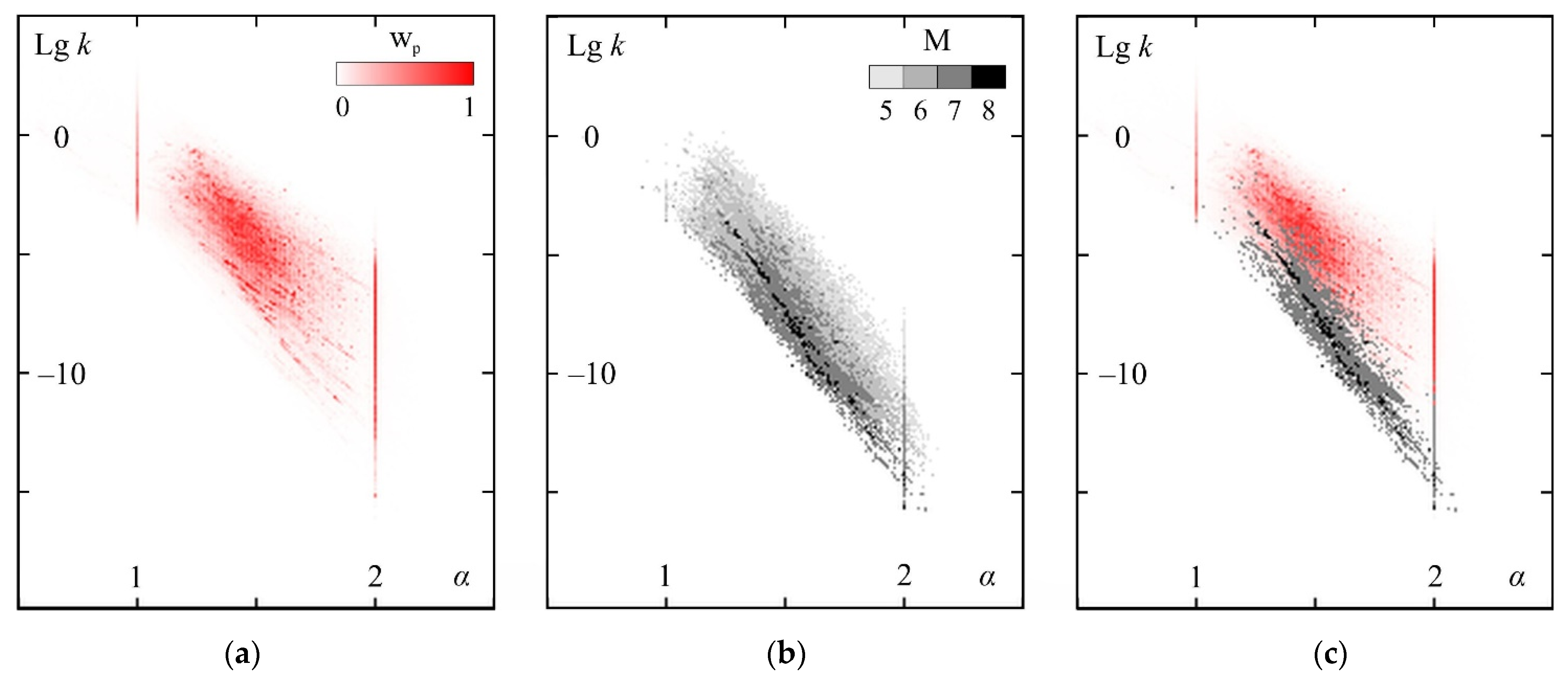
(a) Distribution of the specific weight of predictability wp for activating the seismic energy flux, (b) foreshock predictability of strong earthquakes and (c) their combination in the coordinates of the α–lg k parameters of the DSDNP equation, according to Reference [24]. M is the magnitude of predicted strong earthquakes.
Figure A1.
(a) Distribution of the specific weight of predictability wp for activating the seismic energy flux, (b) foreshock predictability of strong earthquakes and (c) their combination in the coordinates of the α–lg k parameters of the DSDNP equation, according to Reference [24]. M is the magnitude of predicted strong earthquakes.

Figure A1 is constructed in Reference [24] based on the analysis of over 30 million identified best variants of ‘current’ seismicity trends (see Section 2.3). The tendency of increasing the activity in each sequence is checked for extrapolability (predictability). A weight W is assigned to each extrapolation. W = (W1 × W2 × W3)1/3 is the geometric mean of three independent weight characteristics. The first weight component characterizes the forecast range: W1 = [(xp − xs)/(xc − xs) + (tp − ts)/(tc − ts)]/2 − 1. The second weighting component characterizes the nonlinearity of the forecast: W2 = exp|ln[(xp − xs)/(xc − xs))/((tp − ts)/(tc − ts)]| − 1. The third weighting component characterizes the quality of the forecast, i.e., the correspondence of the factual data to the calculated approximation–extrapolation curve: W3 = 0.1/σ − 1; all predictive extrapolations with σ > 0.1 are considered low-quality and rejected. The analysis of the weight distribution of predictive extrapolations by the parameters of the DSDNP equation α and k is carried out with rounding by α with an accuracy of 0.01 and by lg k − up to 0.1. The weights of forecast extrapolations having the same rounded values α and lg k are summed and divided by the total weight of all the forecast extrapolations. Further, these specific weights for all available combinations of α and lg k are sorted in descending order and then summed from smaller values to larger ones. Thus, we obtained a cumulative characteristic of the distribution of a specific weight of wp predictive extrapolations, depending on the combinations of α and lg k: wp(α, lg k) = Σα, lg k(ΣW(α, lg k)/ΣW). wp has values close to 1 at the points of the maximum specific gravity of the forecast extrapolations and close to 0 for combinations of α and lg k that are insignificant from the point of view of the forecast.
The presence of a strong M5+ earthquake was detected in the extrapolation (forecast) part of 315,000 activization sequences. Combinations of the parameters corresponding to these foreshock sequences are shown in Figure A1b. Combinations of the parameters corresponding to 45,636 forecasts for M7+ earthquakes are shown in Figure A1c.
Figure A2.
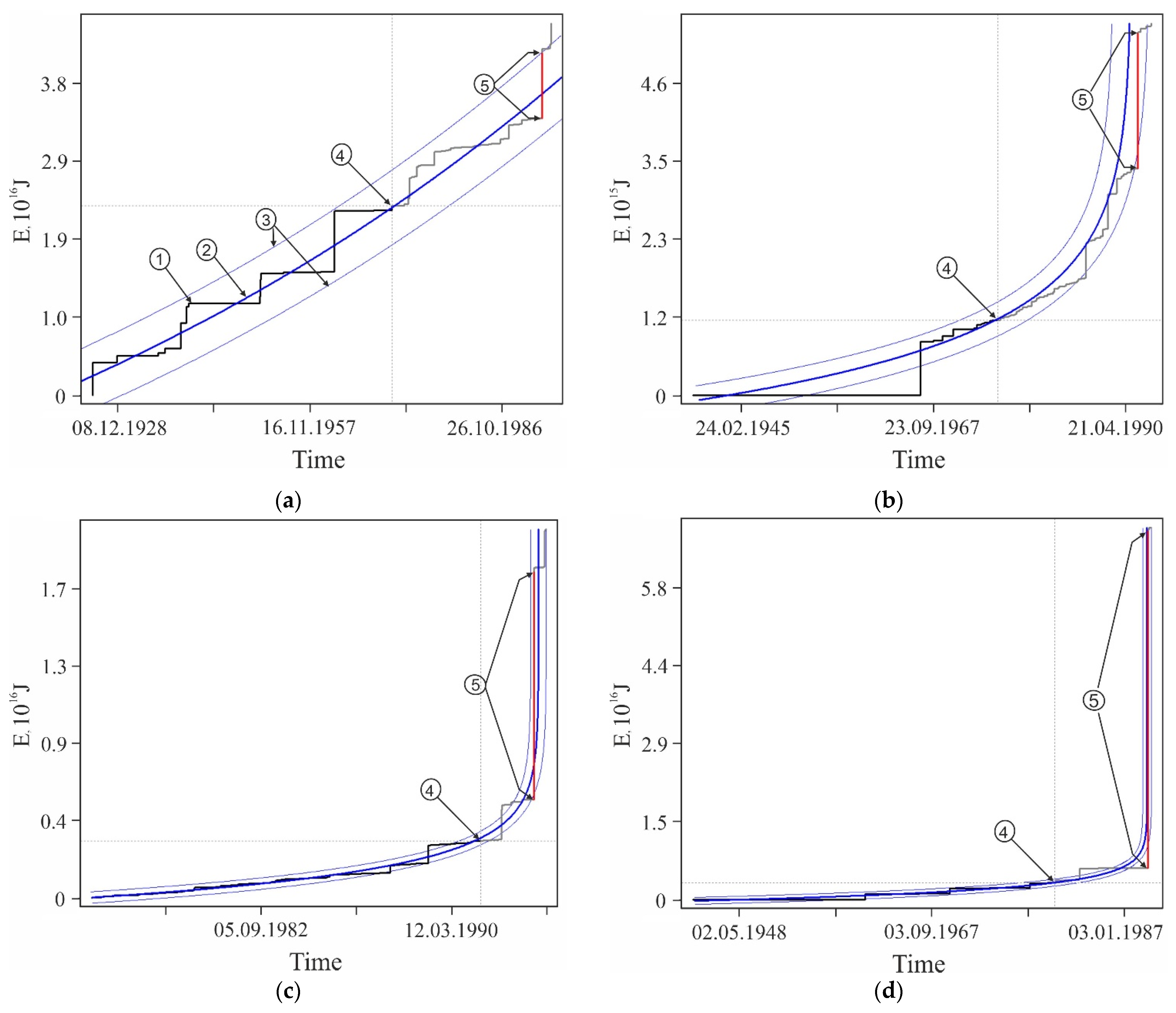
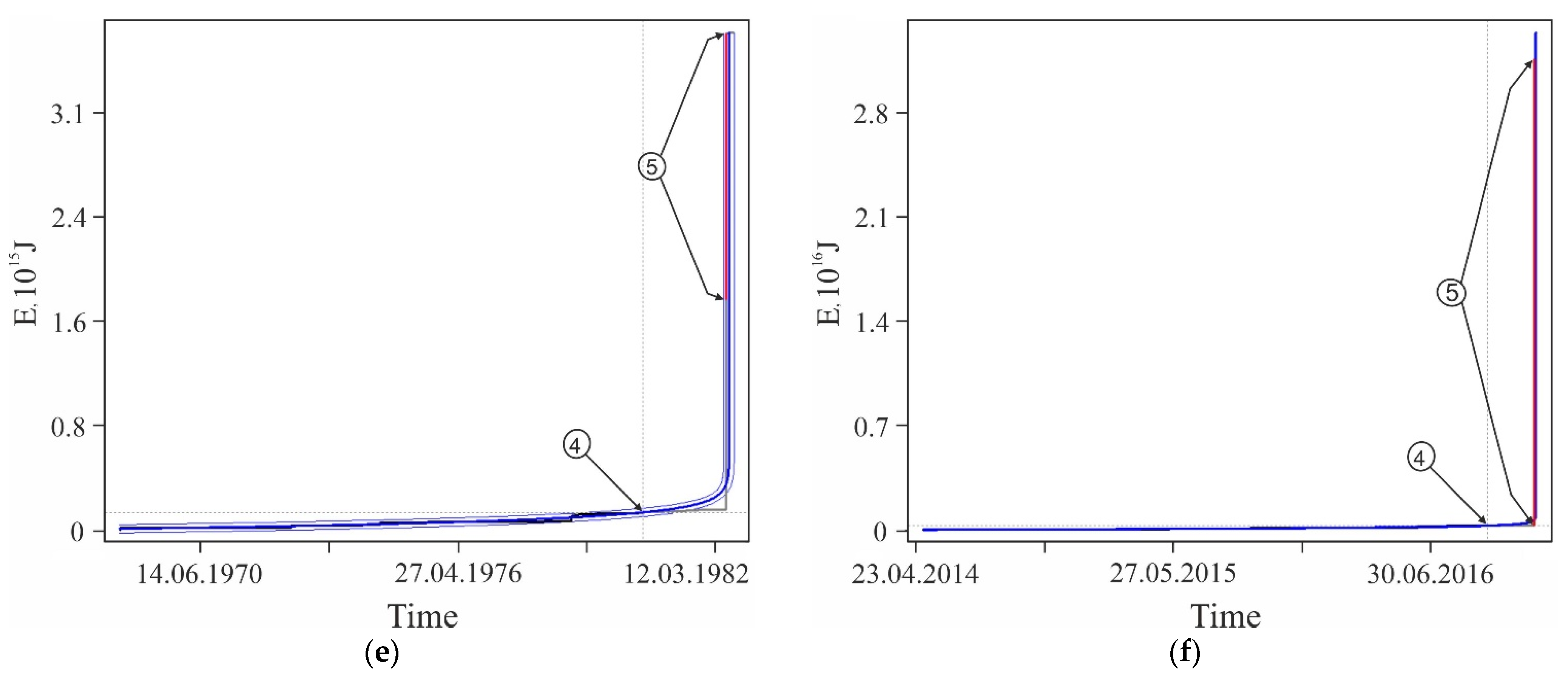
Examples of some foreshock extrapolations of the energy flux. Figures in circles: 1—factual data curve, 2—calculated curve, 3—errors band (±3σ), 4—retrospective prediction moment and 5—strong earthquake. The graphs correspond to the data in Table A1. The intersection of the vertical and horizontal dotted lines on the graphs corresponds to the ‘current’ values of time and parameter, there is the ‘past’ to the left and below this intersection and the ‘future’ to the right and above.
Figure A2.
Examples of some foreshock extrapolations of the energy flux. Figures in circles: 1—factual data curve, 2—calculated curve, 3—errors band (±3σ), 4—retrospective prediction moment and 5—strong earthquake. The graphs correspond to the data in Table A1. The intersection of the vertical and horizontal dotted lines on the graphs corresponds to the ‘current’ values of time and parameter, there is the ‘past’ to the left and below this intersection and the ‘future’ to the right and above.


The graphs in Figure A2 only illustrate the variability of the stochasticity/determinacy of the process, depending on the level of predicted nonlinearity Lpn, but do not prove this statement. Nevertheless, the graphs of all other (27,673—USGS data, 116,420—all catalogs) precedents of the predictability of strong earthquakes demonstrate a similar relationship between Lpn and the band of permissible deviations. All these results (data for graphs) were obtained automatically during catalog processing (see Section 2.3). That is, we did not choose the forecast moments for the graphs in Figure A2. When processing the catalog for each radius of formation of the hypocentral samples, we totally checked all the catalog events. In each case, the event was considered as the ‘current time’ for test approximations and subsequent predictive extrapolations. Among these extrapolations, trends corresponding to successful forecasts of strong earthquakes were automatically detected, including those shown in Figure A2. This made possible and objective the subsequent analysis of the predictability of strong earthquakes. In total, the analysis of the USGS catalog revealed ~18.8 million ‘current’ activation trends. For this purpose, two to three decimal orders of magnitude more test approximations were performed, the results of which were not logged to save computing resources. At the same time, only in 27,673 cases, among the main “current” activation trends, the fact that M7+ earthquakes hit the band of permissible deviations of the extrapolation (prediction) part of the trend was established. We do not consider it necessary to evaluate this result as ‘good’ or ‘bad’. We consider it as an objective reality that can and should be used to identify hazardous activation trends (as it is shown, for example, in Figure A1). The examples for Figure A2 were selected (also automatically) from all other cases of the predictability of strong earthquakes only because each of them has the maximum predictability (by the magnitude of the ratio A) among the forecasts of a certain level of nonlinearity Lpn: Figure A2a—0 < Lpn ≤ 0.5, Figure A2b—0.5 < Lpn ≤ 0.8, Figure A2c—0.9 < Lpn ≤ 0.95, Figure A2d—0.95 < Lpn ≤ 0.98, Figure A2e—0.98 < Lpn ≤ 0.99 and Figure A2c—0.99 < Lpn ≤ 1.0. This corresponds to the sections of the statistical tables. Therefore, examples of Figure A2 can be considered as additional illustrations to Table A2, Table A3 and Table A4. Additionally, when carefully examining the graphs in Figure A2. it can be noticed that the line of actual data in the forecast part of the graphs before a strong earthquake, as a rule, goes beyond the band of permissible deviations and returns to it at the time of the earthquake. This effect is due to the extrapolation estimation algorithm used in the work (see Section 2.4), according to which each of the actual points in the forecast part is consistently monitored for falling into the band of permissible deviations according to the ratio (4). In this case, a variable (increasing) range of rationing is used. Therefore, points that have previously passed the control by the ratio (4) may be outside the tolerance band of subsequent points. The tolerance band for the upper (terminal) point of a strong earthquake is shown in the graphs of Figure A2.

Table A1.
Data on the main shock, sample and some characteristics of the foreshock trend for the examples of retrospective prediction extrapolations given in Figure A2.
Table A1.
Data on the main shock, sample and some characteristics of the foreshock trend for the examples of retrospective prediction extrapolations given in Figure A2.
| (a) | (b) | (c) | (d) | (e) | (f) | ||
|---|---|---|---|---|---|---|---|
| Earthquake | date | 1992 10 11 | 1991 09 30 | 1993 06 08 | 1989 05 23 | 1982 06 07 | 2016 12 08 |
| time | 19:24:26 | 00:21:46 | 13:03:36 | 10:54:46 | 10:59:40 | 17:38:46 | |
| M | 7.4 | 7.0 | 7.5 | 8.0 | 7.0 | 7.8 | |
| latitude | −19.247 | −20.878 | 51.218° | −52.341 | 16.558 | −10.681 | |
| longitude | 168.948 | −178.591 | 157.829 | 158.824 | −98.358 | 161.327 | |
| depth, km | 129 | 566.4 | 70.6 | 10 | 33.8 | 40 | |
| Sample | radius, km | 150 | 60 | 300 | 300 | 150 | 150 |
| latitude | −19.604 | −20.797 | 51.176 | −52.941 | 16.931 | −9.802 | |
| longitude | 168.541 | −178.846 | 159.677 | 158.824 | −97.285 | 160.861 | |
| depth, km | 0 | 600 | 0 | 0 | 100 | 100 | |
| Foreshock trend | tsh_f − tc, days | 8245 | 6001 | 766 | 3312 | 689 | 73.36 |
| Δ = (tsh_f − tc)/σt | 15.90 | 27.34 | 20.33 | 35.32 | 36.28 | 89.22 | |
| Lpn | 0.2313 | 0.7852 | 0.9435 | 0.9757 | 0.9890 | 0.9986 | |
| A | 1.6309 | 2.3451 | 1.9442 | 2.4337 | 2.2048 | 2.1360 | |
| α | 1.0000 | 2.0000 | 2.0000 | 2.0000 | 2.0000 | 2.0000 | |
| lg k | −4.6110 | −15.0095 | −15.2064 | −15.3332 | −13.7995 | −14.0278 |
Table A2.
Distribution of the precedents of foreshock retro-forecasts depending on the sample radius R, predictive nonlinearity Lpn and forecast lead time.
Table A2.
Distribution of the precedents of foreshock retro-forecasts depending on the sample radius R, predictive nonlinearity Lpn and forecast lead time.
| R, km | Lpn | Forecast Lead Time, tsh_f–tc, Days | Total | ||||
|---|---|---|---|---|---|---|---|
| <1 | 1–10 | 10–100 | 100–1000 | >1000 | |||
| 300 | 0.99–1.00 | 1705 | 693 | 1671 | 494 | 2 | 4565 |
| 0.98–0.99 | 2 | 135 | 987 | 1241 | 33 | 2398 | |
| 0.95–0.98 | 1 | 147 | 1752 | 3426 | 406 | 5732 | |
| 0.90–0.95 | 0 | 1 | 1572 | 3281 | 291 | 5145 | |
| 0.80–0.90 | 0 | 0 | 362 | 8819 | 1141 | 10,322 | |
| 0.50–0.80 | 0 | 0 | 14 | 9784 | 6219 | 16,017 | |
| 0.00–0.50 | 0 | 0 | 0 | 401 | 261 | 662 | |
| subtotal | 1708 | 976 | 6358 | 27,446 | 8353 | 44,841 | |
| 150 | 0.99–1.00 | 2072 | 1361 | 1525 | 443 | 10 | 5411 |
| 0.98–0.99 | 2 | 662 | 708 | 914 | 148 | 2434 | |
| 0.95–0.98 | 0 | 983 | 810 | 3085 | 696 | 5574 | |
| 0.90–0.95 | 0 | 249 | 707 | 2773 | 2220 | 5949 | |
| 0.80–0.90 | 0 | 0 | 737 | 4029 | 3099 | 7865 | |
| 0.50–0.80 | 0 | 0 | 1 | 2575 | 3870 | 6446 | |
| 0.00–0.50 | 0 | 0 | 0 | 20 | 252 | 272 | |
| subtotal | 2074 | 3255 | 4488 | 13,839 | 10,295 | 33,951 | |
| 60 | 0.99–1.00 | 3306 | 4775 | 5501 | 858 | 131 | 14,571 |
| 0.98–0.99 | 0 | 18 | 249 | 1186 | 26 | 1479 | |
| 0.95–0.98 | 0 | 13 | 67 | 1559 | 209 | 1848 | |
| 0.90–0.95 | 0 | 0 | 2 | 1384 | 790 | 2176 | |
| 0.80–0.90 | 0 | 0 | 0 | 856 | 1276 | 2132 | |
| 0.50–0.80 | 0 | 0 | 0 | 608 | 897 | 1505 | |
| 0.00–0.50 | 0 | 0 | 0 | 0 | 11 | 11 | |
| subtotal | 3306 | 4806 | 5819 | 6451 | 3340 | 23,722 | |
| 30 | 0.99–1.00 | 3496 | 2494 | 1751 | 738 | 60 | 8539 |
| 0.98–0.99 | 0 | 0 | 7 | 475 | 229 | 711 | |
| 0.95–0.98 | 0 | 0 | 2 | 533 | 313 | 848 | |
| 0.90–0.95 | 0 | 0 | 0 | 114 | 49 | 163 | |
| 0.80–0.90 | 0 | 0 | 0 | 160 | 44 | 204 | |
| 0.50–0.80 | 0 | 0 | 0 | 1 | 8 | 9 | |
| subtotal | 3496 | 2494 | 1760 | 2021 | 703 | 10,474 | |
| 15 | 0.99–1.00 | 1305 | 1202 | 566 | 119 | 20 | 3212 |
| 0.98–0.99 | 1 | 0 | 0 | 0 | 14 | 15 | |
| 0.95–0.98 | 0 | 0 | 0 | 0 | 2 | 2 | |
| 0.90–0.95 | 0 | 0 | 0 | 0 | 2 | 2 | |
| 0.80–0.90 | 0 | 0 | 0 | 0 | 1 | 1 | |
| subtotal | 1306 | 1202 | 566 | 119 | 39 | 3232 | |
| 7.5 | 0.99–1.00 | 468 | 9 | 0 | 3 | 0 | 480 |
| total | 12,358 | 12,742 | 18,991 | 49,879 | 22,730 | 116,700 | |
Table A3.
The maximum (average) relative accuracy Δ of foreshock retro-forecasts depending on the sample radius R, predictive nonlinearity Lpn and forecast lead time.
Table A3.
The maximum (average) relative accuracy Δ of foreshock retro-forecasts depending on the sample radius R, predictive nonlinearity Lpn and forecast lead time.
| R, km | Lpn | Forecast Lead Time, tsh_f–tc, Days | Total | ||||
|---|---|---|---|---|---|---|---|
| <1 | 1–10 | 10–100 | 100–1000 | >1000 | |||
| 300 | 0.99–1.00 | 20.58 (2.38) | 18.63 (1.59) | 27.45 (3.39) | 40.92 (2.67) | 8.63 (8.42) | 40.92 (2.66) |
| 0.98–0.99 | 3.25 (3.24) | 9.89 (3.25) | 25.80 (2.97) | 25.88 (3.22) | 24.53 (15.14) | 25.88 (3.28) | |
| 0.95–0.98 | 4.53 (4.53) | 6.53 (1.98) | 20.27 (2.57) | 22.94 (3.45) | 35.32 (6.43) | 35.32 (3.35) | |
| 0.90–0.95 | 7.63 (7.63) | 8.80 (1.63) | 20.33 (2.75) | 36.33 (5.58) | 36.33 (2.57) | ||
| 0.80–0.90 | 7.51 (1.48) | 18.53 (3.03) | 18.56 (6.60) | 18.56 (3.37) | |||
| 0.50–0.80 | 5.18 (3.75) | 12.51 (3.95) | 23.44 (6.85) | 23.44 (5.08) | |||
| 0.00–0.50 | 8.88 (6.04) | 15.44 (5.46) | 15.44 (5.81) | ||||
| subtotal | 20.58 (2.38) | 18.63 (1.88) | 27.45 (2.55) | 40.92 (3.43) | 36.33 (6.74) | 40.92 (3.85) | |
| 150 | 0.99–1.00 | 24.72 (1.60) | 71.51 (1.71) | 89.22 (3.53) | 37.67 (3.86) | 91.27 (33.64) | 91.27 (2.42) |
| 0.98–0.99 | 3.46 (3.32) | 9.17 (0.51) | 16.25 (3.02) | 36.28 (3.50) | 36.27 (8.27) | 36.28 (2.84) | |
| 0.95–0.98 | 3.32 (0.53) | 10.39 (1.89) | 17.18 (4.89) | 29.12 (4.68) | 29.12 (3.66) | ||
| 0.90–0.95 | 2.86 (1.08) | 5.88 (1.79) | 15.36 (2.73) | 16.46 (4.39) | 16.46 (3.17) | ||
| 0.80–0.90 | 5.87 (2.77) | 16.09 (3.20) | 22.01 (5.09) | 22.01 (3.90) | |||
| 0.50–0.80 | 4.55 (4.55) | 10.36 (3.78) | 20.17 (5.35) | 20.17 (4.72) | |||
| 0.00–0.50 | 4.82 (4.47) | 15.90 (4.57) | 15.90 (4.56) | ||||
| subtotal | 24.72 (1.60) | 71.51 (1.06) | 89.22 (2.75) | 37.67 (3.63) | 91.27 (5.07) | 91.27 (3.58) | |
| 60 | 0.99–1.00 | 21.79 (1.03) | 10.96 (0.97) | 22.18 (2.20) | 59.51 (4.01) | 18.73 (12.20) | 59.51 (1.73) |
| 0.98–0.99 | 2.72 (1.70) | 6.66 (1.87) | 19.29 (2.14) | 17.80 (9.49) | 19.29 (2.22) | ||
| 0.95–0.98 | 2.88 (2.47) | 5.43 (2.32) | 16.69 (2.91) | 18.06 (6.11) | 18.06 (3.25) | ||
| 0.90–0.95 | 1.79 (1.39) | 9.37 (1.84) | 16.37 (5.41) | 16.37 (3.13) | |||
| 0.80–0.90 | 8.98 (2.34) | 18.78 (3.73) | 18.78 (3.17) | ||||
| 0.50–0.80 | 6.75 (3.13) | 28.61 (4.75) | 28.61 (4.10) | ||||
| 0.00–0.50 | 7.53 (4.43) | 7.53 (4.43) | |||||
| subtotal | 21.79 (1.03) | 10.96 0.97) | 22.18 (2.19) | 59.51 (2.63) | 28.61 (4.93) | 59.51 (2.29) | |
| 30 | 0.99–1.00 | 8.61 (1.16) | 12.97 (1.26) | 13.85 (3.75) | 658.60 (3.86) | 22.43 (10.83) | 658.60 (2.02) |
| 0.98–0.99 | 1.53 (0.78) | 8.57 (2.19) | 14.07 (5.68) | 14.07 (3.30) | |||
| 0.95–0.98 | 5.78 (5.76) | 8.35 (2.77) | 11.56 (4.83) | 11.56 (3.53) | |||
| 0.90–0.95 | 9.04 (2.84) | 15.46 (5.84) | 15.46 (3.74) | ||||
| 0.80–0.90 | 6.61 (4.08) | 8.33 (5.46) | 8.33 (4.38) | ||||
| 0.50–0.80 | 5.10 (5.10) | 8.18 (5.68) | 8.18 (5.61) | ||||
| subtotal | 8.61 (1.16) | 12.97 (1.26) | 13.85 (3.74) | 658.60 (3.14) | 22.43 (5.74) | 658.60 (2.31) | |
| 15 | 0.99–1.00 | 10.09 (0.83) | 18.41 (1.40) | 10.13 (5.05) | 31.75 (7.79) | 37.18 (11.34) | 37.18 (2.11) |
| 0.98–0.99 | 5.62 (5.62) | 12.87 (7.02) | 12.87 (6.92) | ||||
| 0.95–0.98 | 12.40 (9.97) | 12.40 (9.97) | |||||
| 0.90–0.95 | 2.40 (2.26) | 2.40 (2.26) | |||||
| 0.80–0.90 | 5.22 (5.22) | 5.22 (5.22) | |||||
| subtotal | 10.09 (0.83) | 18.41 (1.40) | 10.13 (5.05) | 31.75 (7.79) | 37.18 (9.09) | 37.18 (2.14) | |
| 7.5 | 0.99–1.00 | 7.64 (2.00) | 5.77 (3.85) | 9.77 (7.47) | 9.77 (2.07) | ||
| total | 24.72 (1.36) | 71.51 (1.16 | 89.22 (2.67) | 658.60 (3.38) | 91.27 (5.69) | 658.60 (3.26) | |
Table A4.
The maximum (average) approximation–extrapolation relation A of foreshock retro-forecasts depending on the sample radius R, predictive nonlinearity Lpn and forecast lead time.
Table A4.
The maximum (average) approximation–extrapolation relation A of foreshock retro-forecasts depending on the sample radius R, predictive nonlinearity Lpn and forecast lead time.
| R, km | Lpn | Forecast Lead Time, tsh_f–tc, Days | Total | ||||
|---|---|---|---|---|---|---|---|
| <1 | 1–10 | 10–100 | 100–1000 | >1000 | |||
| 300 | 0.99–1.00 | 2.05 (1.82) | 2.26 (1.58) | 2.24 (1.68) | 2.23 (1.60) | 2.06 (2.00) | 2.26 (1.71) |
| 0.98–0.99 | 1.56 (1.56) | 2.15 (1.57) | 2.13 (1.57) | 2.29 (1.61) | 2.18 (2.04) | 2.29 (1.60) | |
| 0.95–0.98 | 1.42 (1.42) | 1.75 (1.47) | 2.12 (1.42) | 2.31 (1.52) | 2.43 (1.83) | 2.43 (1.51) | |
| 0.90–0.95 | 1.60 (1.60) | 1.87 (1.25) | 2.15 (1.36) | 2.36 (1.67) | 2.36 (1.34) | ||
| 0.80–0.90 | 1.68 (1.18) | 2.19 (1.29) | 2.16 (1.53) | 2.19 (1.31) | |||
| 0.50–0.80 | 1.39 (1.26) | 1.84 (1.24) | 2.25 (1.41) | 2.25 (1.30) | |||
| 0.00–0.50 | 1.49 (1.24) | 1.92 (1.23) | 1.92 (1.24) | ||||
| subtotal | 2.05 (1.82) | 2.26 (1.56) | 2.24 (1.46) | 2.31 (1.33) | 2.43 (1.45) | 2.43 (1.39) | |
| 150 | 0.99–1.00 | 2.07 (1.79) | 2.17 (1.61) | 2.22 (1.75) | 2.37 (1.84) | 2.47 (2.21) | 2.47 (1.74) |
| 0.98–0.99 | 1.59 (1.57) | 1.98 (1.24) | 2.15 (1.48) | 2.42 (1.72) | 2.35 (2.07) | 2.42 (1.54) | |
| 0.95–0.98 | 1.54 (1.19) | 2.10 (1.31) | 2.41 (1.67) | 2.27 (1.74) | 2.41 (1.54) | ||
| 0.90–0.95 | 1.32 (1.16) | 1.73 (1.22) | 2.08 (1.40) | 2.40 (1.63) | 2.40 (1.46) | ||
| 0.80–0.90 | 1.70 (1.33) | 2.22 (1.34) | 2.30 (1.53) | 2.30 (1.41) | |||
| 0.50–0.80 | 1.39 (1.39) | 1.71 (1.26) | 2.06 (1.39) | 2.06 (1.34) | |||
| 0.00–0.50 | 1.36 (1.33) | 1.67 (1.23) | 1.67 (1.23) | ||||
| subtotal | 2.07 (1.78) | 2.17 (1.37) | 2.22 (1.48) | 2.42 (1.45) | 2.47 (1.51) | 2.47 (1.49) | |
| 60 | 0.99–1.00 | 2.00 (1.82) | 2.03 (1.74) | 2.19 (1.77) | 2.24 (1.77) | 2.33 (2.16) | 2.33 (1.77) |
| 0.98–0.99 | 1.75 (1.57) | 1.84 (1.44) | 2.11 (1.59) | 2.30 (2.06) | 2.30 (1.58) | ||
| 0.95–0.98 | 1.56 (1.54) | 1.67 (1.42) | 2.24 (1.53) | 2.50 (1.85) | 2.50 (1.56) | ||
| 0.90–0.95 | 1.47 (1.36) | 2.01 (1.36) | 2.22 (1.59) | 2.22 (1.44) | |||
| 0.80–0.90 | 1.80 (1.33) | 2.11 (1.46) | 2.11 (1.41) | ||||
| 0.50–0.80 | 1.60 (1.20) | 2.35 (1.29) | 2.35 (1.25) | ||||
| 0.00–0.50 | 1.61 (1.33) | 1.61 (1.33) | |||||
| subtotal | 2.00 (1.82) | 2.03 (1.74) | 2.19 (1.75) | 2.24 (1.48) | 2.50 (1.50) | 2.50 (1.65) | |
| 30 | 0.99–1.00 | 2.00 (1.84) | 2.02 (1.86) | 2.07 (1.86) | 2.27 (1.81) | 2.19 (2.05) | 2.27 (1.85) |
| 0.98–0.99 | 1.59 (1.36) | 2.06 (1.65) | 2.17 (1.89) | 2.17 (1.73) | |||
| 0.95–0.98 | 1.33 (1.33) | 2.05 (1.62) | 2.15 (1.78) | 2.15 (1.68) | |||
| 0.90–0.95 | 1.84 (1.45) | 2.37 (1.73) | 2.37 (1.53) | ||||
| 0.80–0.90 | 1.69 (1.42) | 1.79 (1.50) | 1.79 (1.44) | ||||
| 0.50–0.80 | 1.47 (1.47) | 1.75 (1.45) | 1.75 (1.45) | ||||
| subtotal | 2.00 (1.84) | 2.02 (1.86) | 2.07 (1.85) | 2.27 (1.67) | 2.37 (1.82) | 2.37 (1.81) | |
| 15 | 0.99–1.00 | 2.00 (1.87) | 2.00 (1.97) | 2.01 (1.98) | 2.19 (1.98) | 2.45 (2.07) | 2.45 (1.93) |
| 0.98–0.99 | 1.70 (1.70) | 2.16 (1.93) | 2.16 (1.91) | ||||
| 0.95–0.98 | 2.13 (2.05) | 2.13 (2.05) | |||||
| 0.90–0.95 | 1.44 (1.41) | 1.44 (1.41) | |||||
| 0.80–0.90 | 1.54 (1.54) | 1.54 (1.54) | |||||
| subtotal | 2.00 (1.87) | 2.00 (1.97) | 2.01 (1.98) | 2.19 (1.98) | 2.45 (1.97) | 2.45 (1.93) | |
| 7.5 | 0.99–1.00 | 2.00 (1.92) | 2.01 (2.00) | 2.01 (2.00) | 2.01 (1.92) | ||
| total | 2.05 (1.82) | 2.26 (1.68) | 2.24 (1.60) | 2.42 (1.40) | 2.50 (1.50) | 2.26 (1.71) | |
Appendix B. Retrospective Cluster Estimates of the Seismic Energy Flux before Some M8+ Earthquakes
M8.0 earthquake (16 November 2000 04:54, latitude −3.980°, longitude 152.169°, depth 33 km).
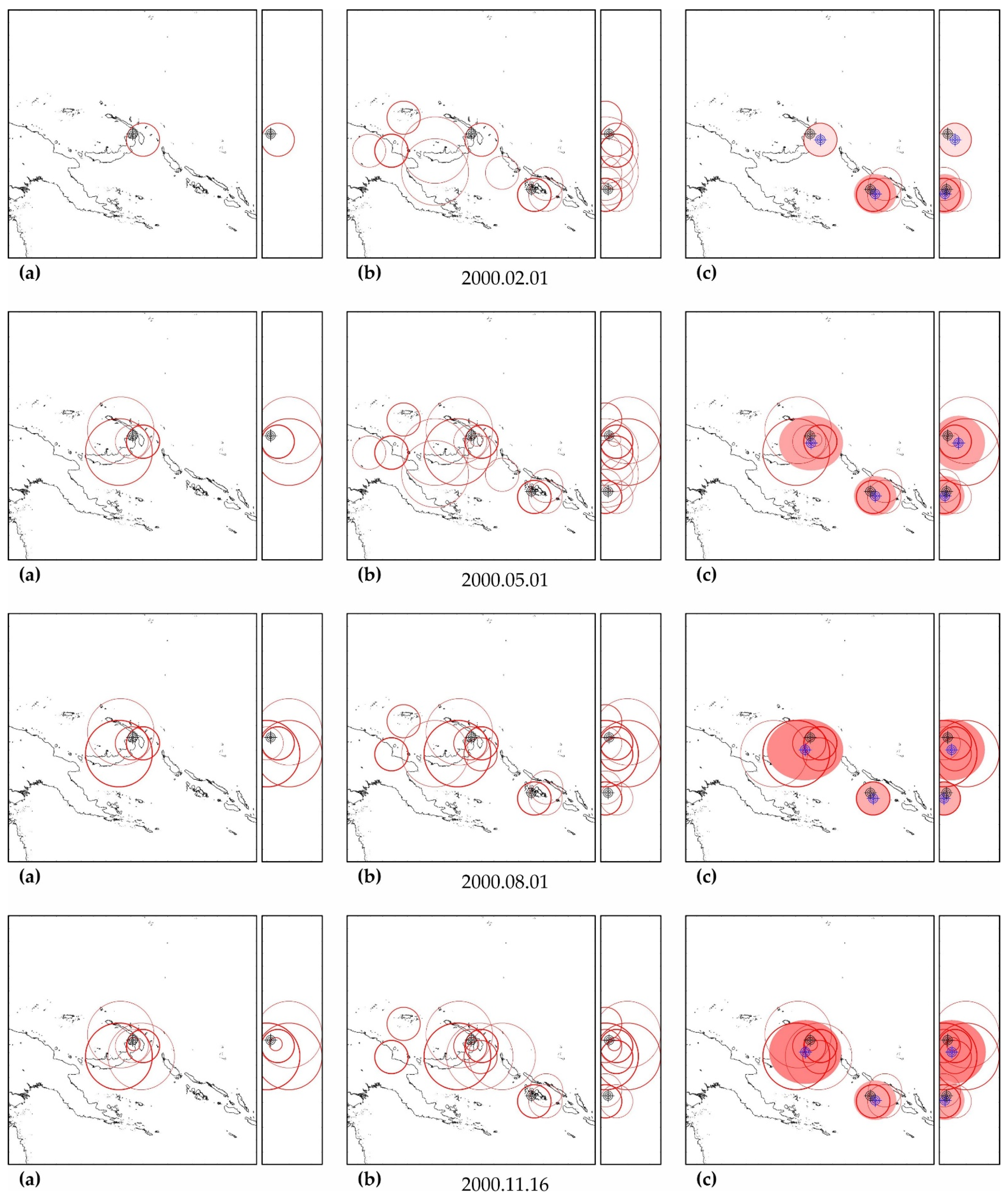
Figure A3.
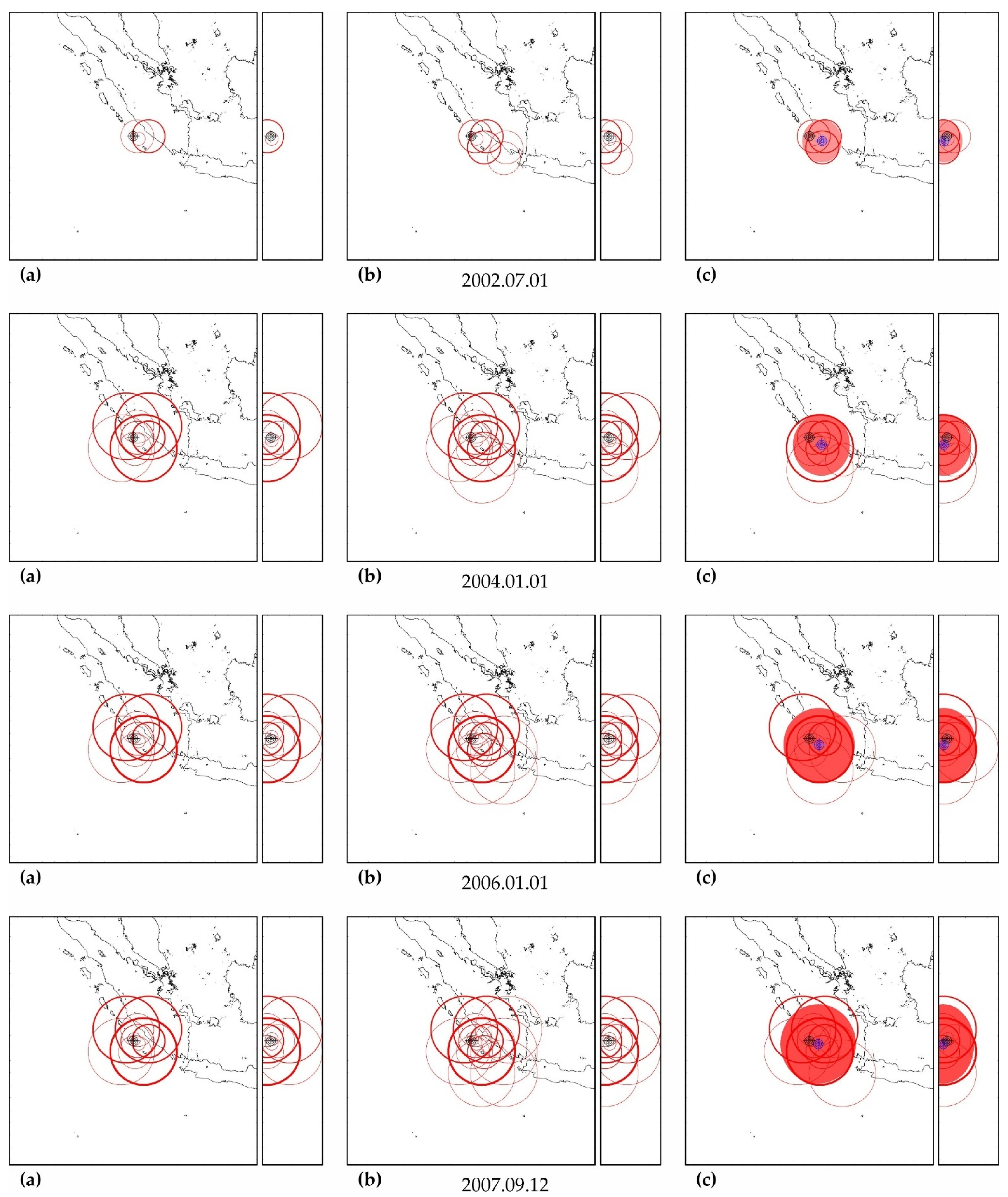
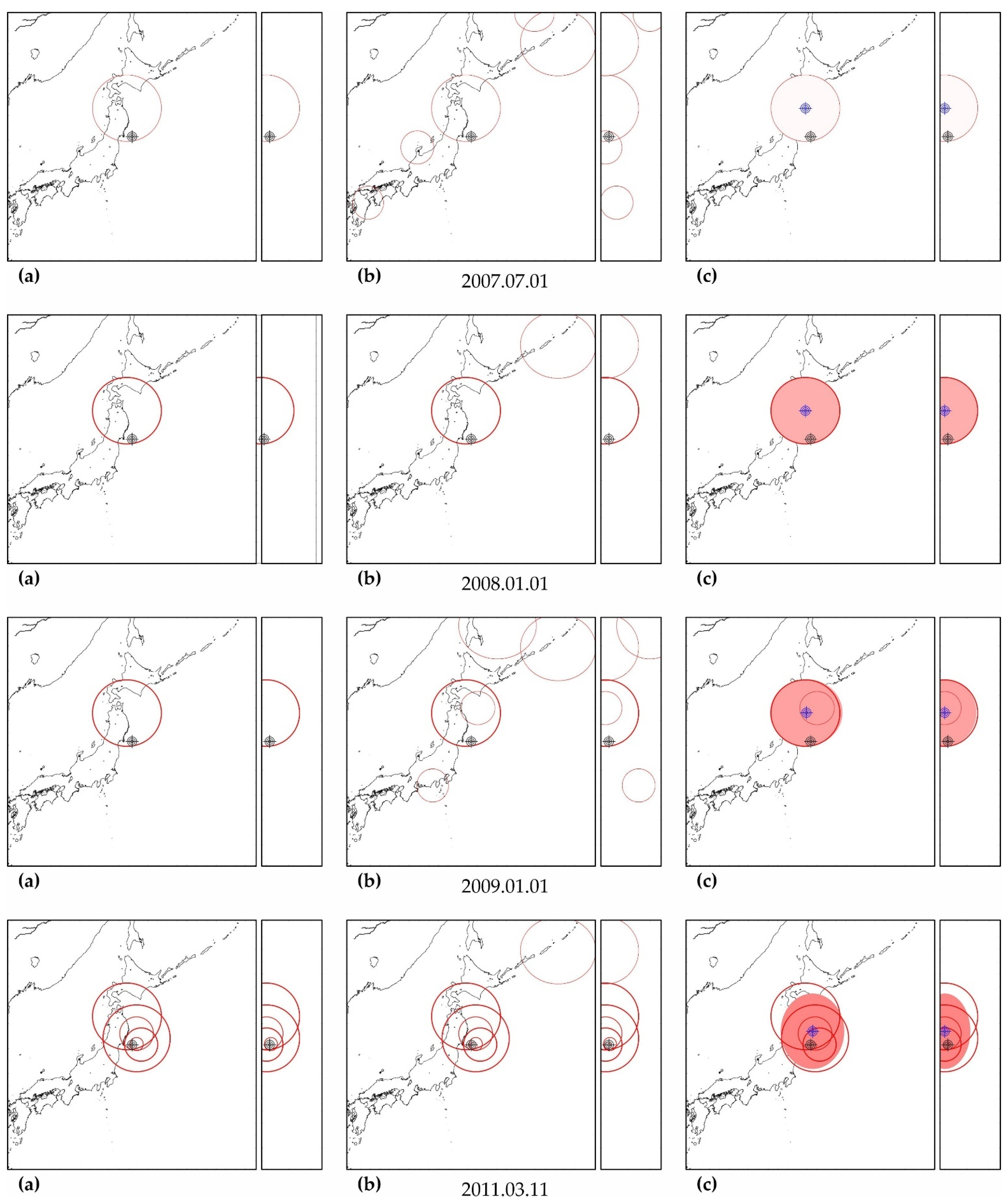
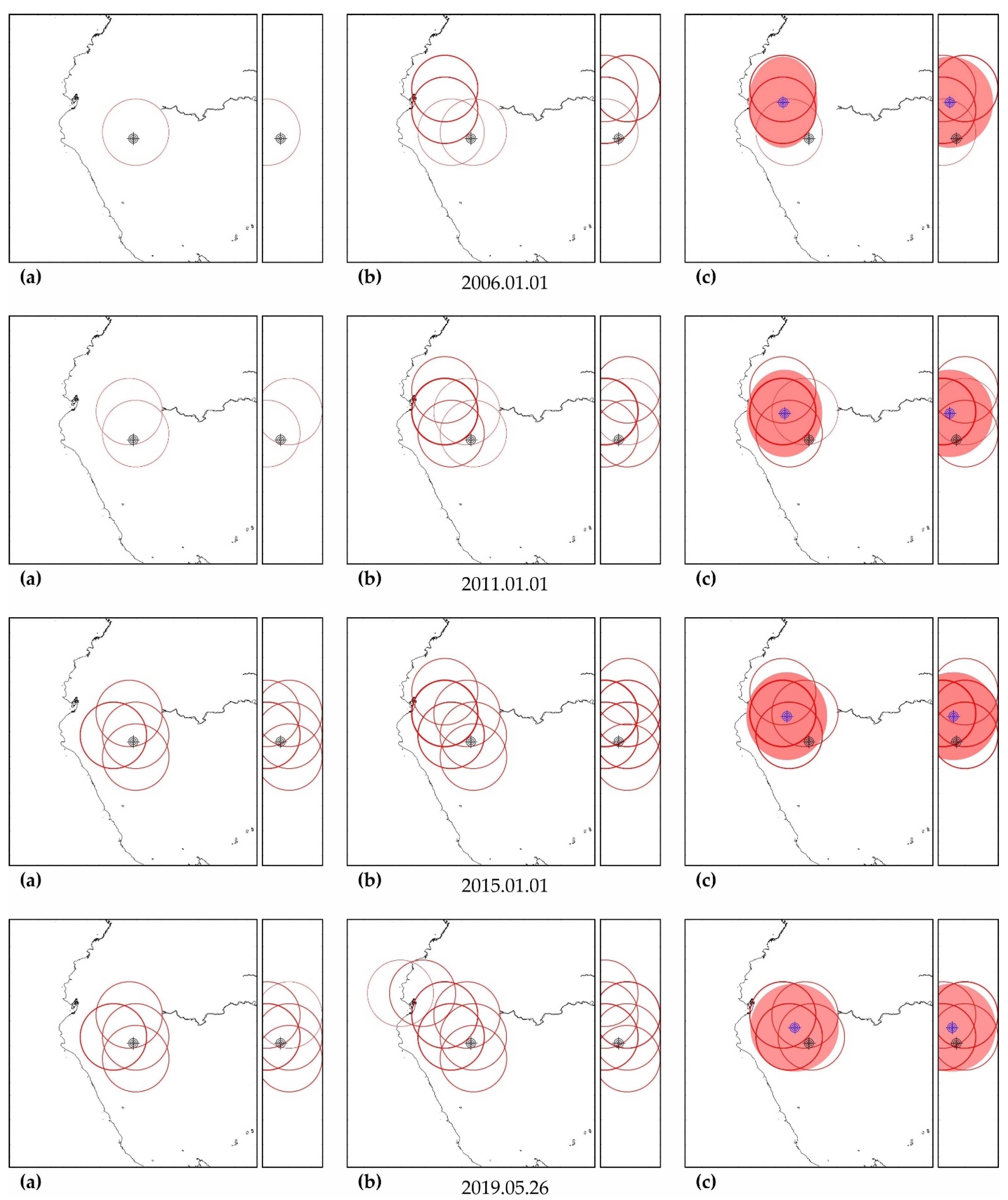
Zones of factual predictability for the earthquake of 16 November 2000 (a), identified zones with similar development according to the parameters of the DSDNP equation (b) and a cluster of zones of the greatest activity (c) used to calculate the time and place of a precedent earthquake. The circles show the position of the zones in which potentially hazardous activity is detected; the thickness of the circle line reflects the number of potentially hazardous trends detected. A double circle with a crosshair is the factual (black) and calculated (blue) positions of the precedent earthquake. The calculated cluster is shown by a solid fill. The cluster color corresponds to the number (the more, the redder) of potentially hazardous unfinished extrapolations found in the cluster. A cluster of predictability of another earthquake (M8.1, 1 April 2007) with a similar foreshock preparation was also found. The size of the maps is 2222 × 2222 km (±10° latitude from the epicenter of the earthquake). The smaller map to the right of each geographical map is a north–south cross-section with a depth of 750 km.
Figure A3.
Zones of factual predictability for the earthquake of 16 November 2000 (a), identified zones with similar development according to the parameters of the DSDNP equation (b) and a cluster of zones of the greatest activity (c) used to calculate the time and place of a precedent earthquake. The circles show the position of the zones in which potentially hazardous activity is detected; the thickness of the circle line reflects the number of potentially hazardous trends detected. A double circle with a crosshair is the factual (black) and calculated (blue) positions of the precedent earthquake. The calculated cluster is shown by a solid fill. The cluster color corresponds to the number (the more, the redder) of potentially hazardous unfinished extrapolations found in the cluster. A cluster of predictability of another earthquake (M8.1, 1 April 2007) with a similar foreshock preparation was also found. The size of the maps is 2222 × 2222 km (±10° latitude from the epicenter of the earthquake). The smaller map to the right of each geographical map is a north–south cross-section with a depth of 750 km.

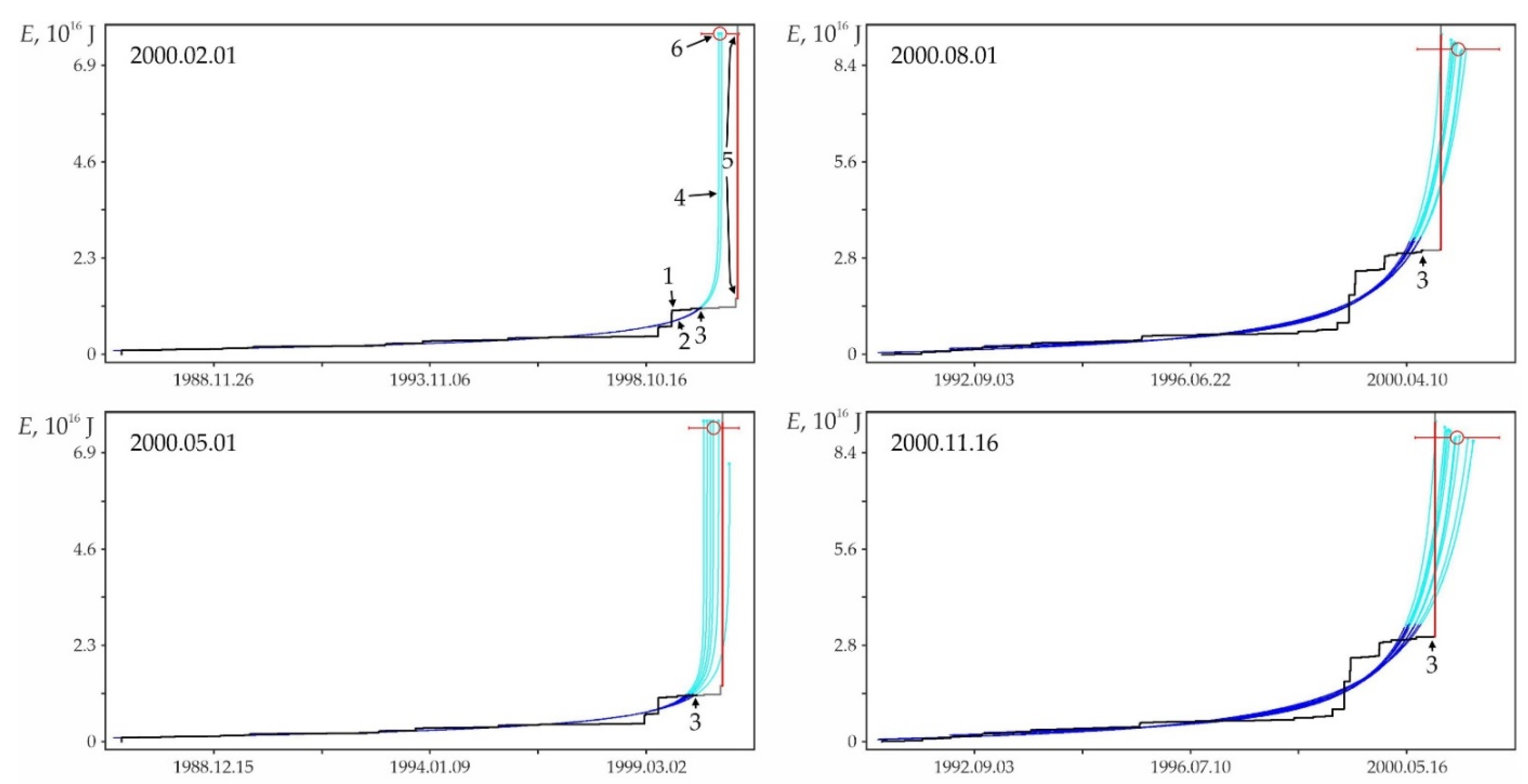
Figure A4.
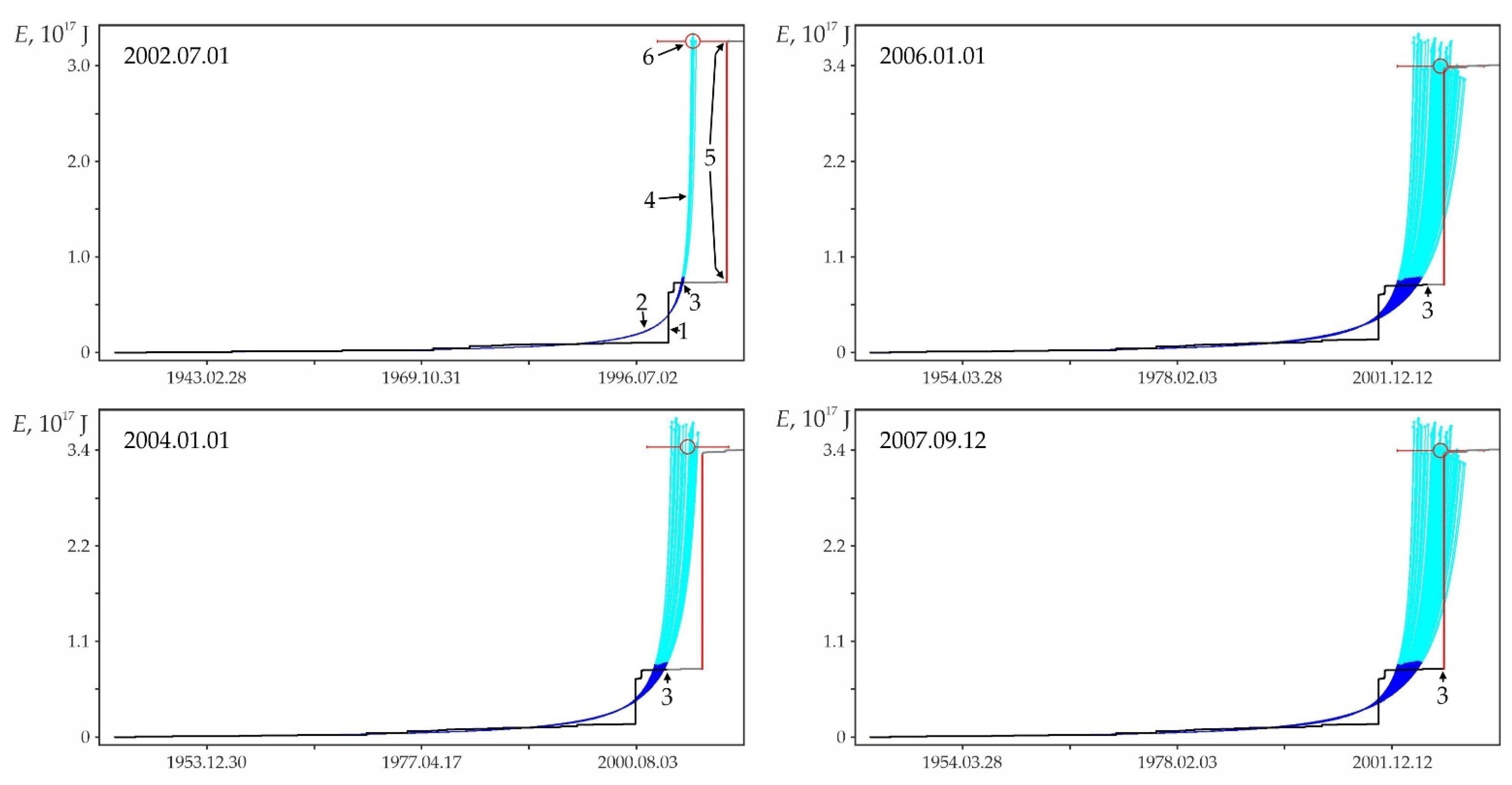
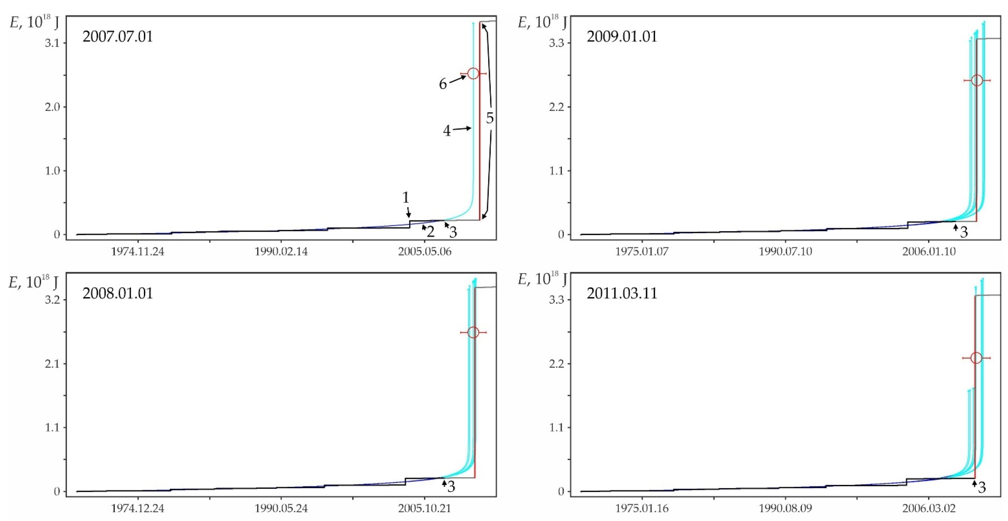
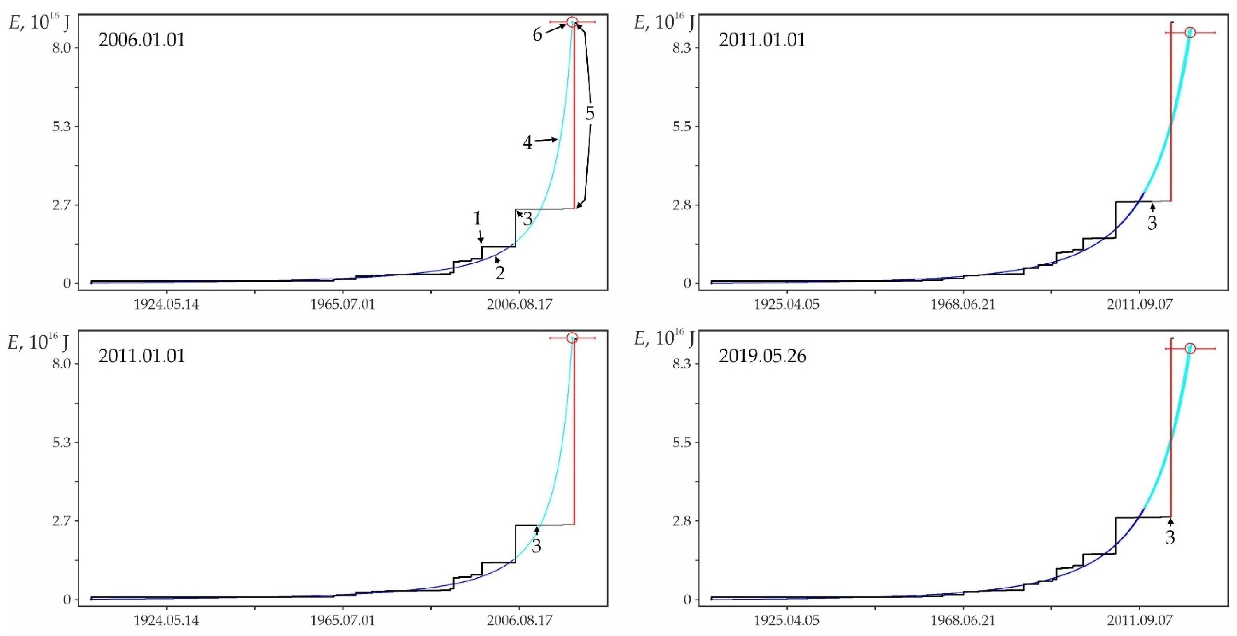
Retro predictability of the earthquake on 16 November 2000 in the zone with the highest (at the estimate date, see Figure A3, column ‘a’) number of successful predictive extrapolations. 1—factual data, 2—approximations, 3—the moment of retro-prediction, 4—extrapolations, 5—the earthquake of 16 November 2000 in factual data and 6—calculation position for the earthquake of 16 November 2000.
Figure A4.
Retro predictability of the earthquake on 16 November 2000 in the zone with the highest (at the estimate date, see Figure A3, column ‘a’) number of successful predictive extrapolations. 1—factual data, 2—approximations, 3—the moment of retro-prediction, 4—extrapolations, 5—the earthquake of 16 November 2000 in factual data and 6—calculation position for the earthquake of 16 November 2000.

Table A5.
Retro estimation of the place and time of earthquakes by clusters of the precedent activity for earthquake 16 November 2000.
Table A5.
Retro estimation of the place and time of earthquakes by clusters of the precedent activity for earthquake 16 November 2000.
| Estimate Date | z | na | npr | Calculated Date | Time Error | Derr, km | |
|---|---|---|---|---|---|---|---|
| Days | % | ||||||
| M8.0 earthquake on 16 November 2000 | |||||||
| 2000.02.01 | 1 | 2 | 2 | 2000.06.23 | 146 | >50 | 126 |
| 2000.03.01 | 6 | 7 | 7 | 2000.07.05 | 134 | >50 | 96 |
| 2000.04.01 | 8 | 10 | 10 | 2000.08.19 | 89 | 38.77 | 113 |
| 2000.05.01 | 8 | 12 | 12 | 2000.09.16 | 60 | 30.23 | 119 |
| 2000.06.01 | 11 | 16 | 16 | 2000.10.28 | 19 | 11.12 | 105 |
| 2000.07.01 | 11 | 21 | 27 | 2000.12.12 | 27 | 16.23 | 109 |
| 2000.08.01 | 12 | 26 | 32 | 2001.01.17 | 62 | 36.69 | 125 |
| 2000.09.01 | 10 | 27 | 35 | 2001.02.23 | 99 | >50 | 121 |
| 2000.10.01 | 10 | 27 | 35 | 2001.03.06 | 110 | >50 | 122 |
| 2000.11.16 | 10 | 32 | 40 | 2001.03.03 | 107 | >50 | 121 |
| M8.1 earthquake on 1 April 2007 (20:39:58, −8.466°, 157.043°, 24 km) | |||||||
| 2000.02.01 | 3 | 11 | 11 | 2005.04.18 | 713 | 27.26 | 62 |
| 2000.03.01 | 3 | 11 | 11 | 2005.04.18 | 713 | 27.57 | 62 |
| 2000.04.01 | 3 | 11 | 11 | 2005.04.18 | 713 | 27.90 | 62 |
| 2000.05.01 | 3 | 11 | 11 | 2005.04.18 | 713 | 28.23 | 62 |
| 2000.06.01 | 3 | 11 | 11 | 2005.04.18 | 713 | 28.58 | 62 |
| 2000.07.01 | 3 | 11 | 11 | 2005.04.18 | 713 | 28.93 | 62 |
| 2000.08.01 | 1 | 9 | 9 | 2006.08.30 | 214 | 8.79 | 61 |
| 2000.09.01 | 1 | 9 | 9 | 2006.08.30 | 214 | 8.91 | 61 |
| 2000.10.01 | 1 | 9 | 9 | 2006.08.30 | 214 | 9.02 | 61 |
| 2000.11.16 | 3 | 11 | 11 | 2005.04.18 | 713 | 30.64 | 62 |
Note. z—number of zones in the cluster, na—the number of unfinished predictive extrapolations in the cluster and npr—the number of precedent time calculations.
M8.1 earthquake (23 January 2007 04:23, latitude 46.243°, longitude 154.524°, depth 10 km).
Figure A5.
Zones of factual predictability for the earthquake of 13 January 2007 (a), identified zones with similar development according to the parameters of the DSDNP equation (b) and a cluster of zones of the greatest activity (c) used to calculate the time and place of a precedent earthquake (see Figure A3 for explanations).

Figure A6.
Retro predictability of the earthquake on 13 January 2007 in the zone with the highest (at the estimate date; see Figure A5, column ‘a’) number of successful predictive extrapolations (see Figure A4 for explanations).

Table A6.
Retro estimation of the place and time of the earthquake on 13 January 2007 by the cluster of its precedent activity.
Table A6.
Retro estimation of the place and time of the earthquake on 13 January 2007 by the cluster of its precedent activity.
| Estimate Date | z | na | npr | Calculated Date | Time Error | Derr, km | |
|---|---|---|---|---|---|---|---|
| Days | % | ||||||
| 2006.12.01 | 2 | 3 | 3 | 2006.11.30 | 44 | >50 | 34 |
| 2006.12.16 | 13 | 21 | 34 | 2006.12.12 | 32 | >50 | 14 |
| 2007.01.01 | 10 | 31 | 55 | 2006.12.27 | 16 | >50 | 40 |
| 2007.01.13 | 13 | 38 | 66 | 2006.12.30 | 13 | >50 | 41 |
M8.4 earthquake (12 September 2007 11:10, latitude −4.438°, longitude 101.367°, depth 34 km).
Figure A7.
Zones of factual predictability for the earthquake of 12 September 2007 (a), identified zones with similar development according to the parameters of the DSDNP equation (b) and a cluster of zones of the greatest activity (c) used to calculate the time and place of a precedent earthquake (see Figure A3 for explanations).

Figure A8.
Retro predictability of the earthquake on 12 September 2007 in the zone with the highest (at the estimate date; see Figure A7, column ‘a’) number of successful predictive extrapolations (see Figure A4 for explanations).

Table A7.
Retro estimation of the place and time of the earthquake on 12 September 2007 by the cluster of its precedent activity.
Table A7.
Retro estimation of the place and time of the earthquake on 12 September 2007 by the cluster of its precedent activity.
| Estimate Date | z | na | npr | Calculated Date | Time Error | Derr, km | |
|---|---|---|---|---|---|---|---|
| days | % | ||||||
| 2002.07.01 | 6 | 19 | 30 | 2003.07.02 | 1533 | >50 | 124 |
| 2003.01.01 | 12 | 34 | 108 | 2004.07.24 | 1145 | >50 | 97 |
| 2004.01.01 | 15 | 90 | 299 | 2005.10.30 | 682 | >50 | 131 |
| 2005.01.01 | 17 | 139 | 605 | 2007.01.09 | 246 | 25.02 | 129 |
| 2006.01.01 | 18 | 147 | 656 | 2007.02.11 | 213 | 34.44 | 106 |
| 2007.01.01 | 19 | 151 | 584 | 2007.01.12 | 243 | >50 | 121 |
| 2007.09.12 | 21 | 177 | 764 | 2007.02.17 | 207 | >50 | 90 |
M9.1 earthquake (11 March 2011 05:46, latitude 38.297°, longitude 142.373°, depth 29 km).
Figure A9.
Zones of factual predictability for the earthquake of 11 March 2011 (a), identified zones with similar development according to the parameters of the DSDNP equation (b) and a cluster of zones of the greatest activity (c) used to calculate the time and place of a precedent earthquake (see Figure A3 for explanations).

Figure A10.
Retro predictability of the earthquake on 11 March 2011 in the zone with the highest (at the estimate date; see Figure A9, column ‘a’) number of successful predictive extrapolations (see Figure A4 for explanations).

Table A8.
Retro estimation of the place and time of the earthquake on 11 March 2011 by the cluster of its precedent activity.
Table A8.
Retro estimation of the place and time of the earthquake on 11 March 2011 by the cluster of its precedent activity.
| Estimate Date | z | na | npr | Calculated Date | Time Error | Derr, km | |
|---|---|---|---|---|---|---|---|
| days | % | ||||||
| 2007.07.01 | 1 | 1 | 9 | 2010.06.30 | 253 | 18.78 | 261 |
| 2008.01.01 | 1 | 9 | 81 | 2011.01.13 | 56 | 4.85 | 261 |
| 2009.01.01 | 2 | 13 | 109 | 2011.04.01 | 21 | 2.58 | 263 |
| 2010.01.01 | 1 | 12 | 108 | 2011.04.08 | 28 | 6.15 | 261 |
| 2011.01.01 | 1 | 12 | 99 | 2011.04.27 | 47 | 40.39 | 261 |
| 2011.03.01 | 1 | 12 | 93 | 2011.05.02 | 53 | >50 | 261 |
| 2011.03.11 | 7 | 31 | 115 | 2011.04.22 | 43 | >50 | 126 |
M8.0 earthquake (6 February 2013 01:12, latitude −10.799°, longitude 165.114°, depth 24 km).
Figure A11.
Zones of factual predictability for the earthquake of 6 February 2013 (a), identified zones with similar development according to the parameters of the DSDNP equation (b) and a cluster of zones of the greatest activity (c) used to calculate the time and place of a precedent earthquake (see Figure A3 for explanations). Clusters of predictability of other earthquakes (9 January 2001 M7.1, 1 April 2007 M8.1 and 10 August 2010 M7.3) were also found with similar preparations.

Figure A12.
Retro predictability of the earthquake on 6 February 2013 in the zone with the highest (at the estimate date; see Figure A11, column ‘a’) number of successful predictive extrapolations (see Figure A4 for explanations).
Figure A12.
Retro predictability of the earthquake on 6 February 2013 in the zone with the highest (at the estimate date; see Figure A11, column ‘a’) number of successful predictive extrapolations (see Figure A4 for explanations).

Table A9.
Retro estimation of the place and time of earthquakes by clusters of precedent activity for earthquake 6 February 2013.
Table A9.
Retro estimation of the place and time of earthquakes by clusters of precedent activity for earthquake 6 February 2013.
| Estimate Date | z | na | npr | Calculated Date | Time Error | Derr, km | |
|---|---|---|---|---|---|---|---|
| Days | % | ||||||
| M8.0 earthquake on 6 February 2013 | |||||||
| 2001.01.01 | 3 | 4 | 6 | 2005.10.07 | 132 | >50 | 2679 |
| 2002.01.01 | 3 | 4 | 6 | 2005.10.07 | 132 | >50 | 2679 |
| 2003.01.01 | 3 | 4 | 6 | 2005.10.07 | 132 | >50 | 2679 |
| 2004.01.01 | 2 | 3 | 5 | 2006.04.26 | 132 | >50 | 2477 |
| 2005.01.01 | 3 | 3 | 4 | 2009.07.23 | 80 | 43.72 | 1293 |
| 2006.01.01 | 4 | 3 | 4 | 2009.07.23 | 80 | 49.87 | 1293 |
| 2007.01.01 | 2 | 2 | 2 | 2012.12.22 | 33 | 2.05 | 46 |
| 2008.01.01 | 2 | 2 | 2 | 2012.12.22 | 33 | 2.45 | 46 |
| 2009.01.01 | 2 | 2 | 2 | 2012.12.22 | 33 | 3.05 | 46 |
| 2010.01.01 | 2 | 2 | 2 | 2012.12.22 | 33 | 4.03 | 46 |
| 2011.01.01 | 1 | 1 | 1 | 2015.07.29 | 27 | >50 | 904 |
| 2012.01.01 | 2 | 3 | 6 | 2013.01.21 | 112 | 3.86 | 16 |
| 2013.01.01 | 3 | 5 | 11 | 2013.10.05 | 102 | >50 | 241 |
| 2013.02.06 | 11 | 17 | 23 | 2013.06.01 | 28 | >50 | 116 |
| M7.1 earthquake on 9 January 2001 (16:49:28, −14.928°, 167.170°, 103 km) | |||||||
| 2001.01.01 | 1 | 2 | 3 | 2000.09.03 | 176 | >50 | 129 |
| M8.1 earthquake on 1 April 2007 (20:39:58, −8.466°, 157.043°, 24 km) | |||||||
| 2001.01.01 | 2 | 8 | 16 | 2005.08.19 | 171 | 25.86 | 590 |
| 2002.01.01 | 3 | 9 | 17 | 2005.06.02 | 188 | 34.86 | 668 |
| 2003.01.01 | 2 | 8 | 16 | 2005.08.19 | 171 | 38.03 | 590 |
| 2004.01.01 | 2 | 7 | 14 | 2005.11.25 | 162 | 41.50 | 492 |
| 2005.01.01 | 2 | 7 | 14 | 2005.11.25 | 162 | >50 | 492 |
| 2006.01.01 | 2 | 6 | 12 | 2005.12.15 | 151 | >50 | 473 |
| 2007.01.01 | 2 | 4 | 8 | 2006.07.11 | 158 | >50 | 264 |
| M7.3 earthquake on 10 August 2010 (05:23:44, −17.541°, 168.069°, 25 km) | |||||||
| 2003.01.01 | 2 | 4 | 5 | 2005.03.18 | 71 | >50 | 1971 |
| 2004.01.01 | 3 | 12 | 13 | 2005.10.15 | 37 | >50 | 1760 |
| 2005.01.01 | 4 | 18 | 18 | 2006.05.23 | 24 | >50 | 1540 |
| 2006.01.01 | 4 | 18 | 18 | 2006.05.23 | 24 | >50 | 1540 |
M8.2 earthquake (1 April 2014 23:46, latitude −19.610°, longitude −70.769°, depth 25 km).
Figure A13.
Zones of factual predictability for the earthquake of 1 April 2014 (a), identified zones with similar development according to the parameters of the DSDNP equation (b) and a cluster of zones of the greatest activity (c) used to calculate the time and place of a precedent earthquake (see Figure A3 for explanations).

Figure A14.
Retro predictability of the earthquake on 1 April 2014 in the zone with the highest (at the estimate date; see Figure A13, column ‘a’) number of successful predictive extrapolations (see Figure A4 for explanations).
Figure A14.
Retro predictability of the earthquake on 1 April 2014 in the zone with the highest (at the estimate date; see Figure A13, column ‘a’) number of successful predictive extrapolations (see Figure A4 for explanations).

Table A10.
Retro estimation of the place and time of the earthquake on 1 April 2014 by the cluster of its precedent activity.
Table A10.
Retro estimation of the place and time of the earthquake on 1 April 2014 by the cluster of its precedent activity.
| Estimate Date | z | na | npr | Calculated Date | Time Error | Derr, km | |
|---|---|---|---|---|---|---|---|
| Days | % | ||||||
| 2005.01.01 | 6 | 12 | 15 | 2006.12.27 | 2653 | >50 | 50 |
| 2006.01.01 | 5 | 33 | 60 | 2016.01.16 | 655 | 17.85 | 218 |
| 2007.01.01 | 6 | 36 | 66 | 2016.06.28 | 818 | 23.60 | 215 |
| 2008.01.01 | 4 | 26 | 126 | 2008.10.14 | 1995 | >50 | 288 |
| 2009.01.01 | 9 | 50 | 310 | 2009.03.28 | 1831 | >50 | 271 |
| 2010.01.01 | 6 | 57 | 180 | 2009.09.23 | 1652 | >50 | 258 |
| 2011.01.01 | 11 | 117 | 485 | 2011.10.14 | 900 | >50 | 153 |
| 2012.01.01 | 12 | 142 | 601 | 2012.08.31 | 579 | >50 | 152 |
| 2013.01.01 | 10 | 132 | 613 | 2013.01.04 | 453 | >50 | 139 |
| 2014.01.01 | 7 | 121 | 509 | 2014.06.10 | 70 | 43.45 | 110 |
| 2014.04.01 | 18 | 164 | 651 | 2014.06.14 | 74 | >50 | 76 |
M8.0 earthquake (26 May 2019 07:41, latitude −5.812°, longitude −75.270°, depth 122 km).
Figure A15.
Zones of factual predictability for the earthquake of 26 May 2019 (a), identified zones with similar development according to the parameters of the DSDNP equation (b) and a cluster of zones of the greatest activity (c) used to calculate the time and place of a precedent earthquake (see Figure A3 for explanations).

Figure A16.
Retro predictability of the earthquake on 26 May 2019 in the zone with the highest (at the estimate date; see Figure A15, column ‘a’) number of successful predictive extrapolations (see Figure A4 for explanations).
Figure A16.
Retro predictability of the earthquake on 26 May 2019 in the zone with the highest (at the estimate date; see Figure A15, column ‘a’) number of successful predictive extrapolations (see Figure A4 for explanations).

Table A11.
Retro estimation of the place and time of the earthquake on 26 May 2019 by the cluster of its precedent activity.
Table A11.
Retro estimation of the place and time of the earthquake on 26 May 2019 by the cluster of its precedent activity.
| Estimate Date | z | na | npr | Calculated Date | Time Error | Derr, km | |
|---|---|---|---|---|---|---|---|
| Days | % | ||||||
| 2006.01.01 | 4 | 22 | 42 | 2009.04.12 | 3696 | >50 | 405 |
| 2007.01.01 | 4 | 21 | 41 | 2009.06.19 | 3628 | >50 | 407 |
| 2008.01.01 | 6 | 21 | 45 | 2009.12.06 | 3458 | >50 | 382 |
| 2009.01.01 | 5 | 25 | 55 | 2010.03.17 | 3356 | >50 | 376 |
| 2010.01.01 | 4 | 25 | 61 | 2011.09.02 | 2823 | >50 | 336 |
| 2011.01.01 | 7 | 26 | 66 | 2012.10.22 | 2407 | >50 | 330 |
| 2012.01.01 | 7 | 23 | 59 | 2013.04.25 | 2222 | >50 | 320 |
| 2013.01.01 | 7 | 29 | 75 | 2015.08.25 | 1369 | >50 | 287 |
| 2014.01.01 | 6 | 34 | 93 | 2016.04.21 | 1130 | >50 | 287 |
| 2015.01.01 | 9 | 31 | 83 | 2015.04.29 | 1487 | >50 | 305 |
| 2016.01.01 | 9 | 29 | 79 | 2017.07.12 | 683 | >50 | 269 |
| 2017.01.01 | 9 | 22 | 62 | 2018.09.27 | 241 | 27.50 | 267 |
| 2018.01.01 | 8 | 16 | 46 | 2020.02.03 | 253 | 33.12 | 240 |
| 2019.01.01 | 8 | 15 | 42 | 2020.11.14 | 539 | >50 | 246 |
| 2019.05.26 | 9 | 19 | 45 | 2021.03.09 | 653 | >50 | 195 |
Appendix C. Current Cluster Estimates of the Potential Hazard of Seismic Energy Flux
Figure A17.
Cluster estimates of the potential hazard of seismic energy flux: 1 January 2020 (a), 1 July 2020 (b), 1 January 2021 (c) and 1 June 2021 (d). The cluster color corresponds to the number (the more, the redder) of potentially hazardous unfinished extrapolations found in the cluster. Circles with a crosshair are M7+ earthquakes that occurred after the hazard assessment date before 1 June 2021: black—in identified activity clusters and within the error band of predicted trends (full predictability, Table A12), green—in identified activity clusters with a violation of the error band of trends in the cluster (partially predictability) and blue—unrelated to clusters of potentially hazardous activity (lack of predictability).

Table A12.
M7+ earthquakes that occurred during the period after the hazard estimation until 1 June 2021 in accordance with the extrapolation of trends in the identified clusters.
Table A12.
M7+ earthquakes that occurred during the period after the hazard estimation until 1 June 2021 in accordance with the extrapolation of trends in the identified clusters.
| Earthquake | Number of Successful Extrapolations | ||||||
|---|---|---|---|---|---|---|---|
| Date | Latitude | Longitude | Depth | M | 1 January 2020 | 1 July 2020 | 1 January 2021 |
| 2020.07.22 | 55.072 | −158.596 | 28.0 | 7.8 | 4 | 4 | |
| 2020.10.30 | 37.897 | 26.784 | 21.0 | 7.0 | 3 | 3 | |
| 2021.02.10 | −23.051 | 171.657 | 10.0 | 7.7 | 9 | 12 | 15 |
| 2021.02.13 | 37.727 | 141.775 | 44.0 | 7.1 | 13 | 13 | 12 |
| 2021.03.04 | −37.479 | 179.458 | 10.0 | 7.3 | 11 | 11 | 11 |
| 2021.03.04 | −29.677 | −177.840 | 43.0 | 7.4 | 2 | 3 | |
| 2021.03.04 | −29.723 | −177.279 | 28.9 | 8.1 | 2 | 2 | 2 |
Table A13.
Main clusters of hazardous activity as of 1 June 2021.
| No. | Localization | Precedent Earthquake | Extrapolation Calculations | |||||||||||||
|---|---|---|---|---|---|---|---|---|---|---|---|---|---|---|---|---|
| Latitude | Longitude | Depth | R, km | Catalogue | M | Date | Latitude | Longitude | Depth | z | na | npr | Date | σsh | σt | |
| 1 | 60.778 | −150.661 | 29 | 156.8 | JMA | 8.2 | 2007.01.13 | 46.938 | 155.052 | 30.0 | 9 | 659 | 1591 | 2021.10.11 | 339 | 78 |
| 2 | 35.703 | −118.052 | 0 | 150.0 | JMA | 8.2 | 2007.01.13 | 46.938 | 155.052 | 30.0 | 3 | 632 | 2089 | 2021.04.22 | 84 | 107 |
| 3 | 62.373 | −149.723 | 23 | 300.0 | USGS | 8.3 | 1994.10.04 | 43.773 | 147.321 | 14.0 | 3 | 174 | 174 | 2023.03.07 | 205 | 21 |
| 4 | 36.315 | −97.421 | 0 | 300.0 | JMA | 8.2 | 1994.10.04 | 43.375 | 147.673 | 28.0 | 3 | 166 | 166 | 2023.06.09 | 184 | 4 |
| 5 | 56.168 | −149.196 | 0 | 152.1 | USGS | 8.0 | 2000.11.16 | −3.980 | 152.169 | 33.0 | 3 | 144 | 144 | 2018.10.31 | 99 | 353 |
| 6 | 63.315 | −150.986 | 33 | 271.3 | USGS | 8.0 | 2000.11.16 | −3.980 | 152.169 | 33.0 | 5 | 142 | 142 | 2023.04.20 | 298 | 79 |
| 7 | 60.135 | −152.369 | 66 | 150.0 | USGS | 8.6 | 2005.03.28 | 2.085 | 97.108 | 30.0 | 4 | 134 | 134 | 2023.03.05 | 517 | 47 |
| 8 | 60.000 | −146.939 | 0 | 300.0 | JMA | 8.0 | 2003.09.26 | 41.779 | 144.078 | 45.1 | 1 | 120 | 1048 | 2020.11.02 | 77 | 107 |
| 9 | 56.379 | −150.343 | 0 | 300.0 | USGS | 8.0 | 2019.05.26 | −5.812 | −75.270 | 122.6 | 2 | 115 | 293 | 2021.01.15 | 183 | 1742 |
| 10 | 56.497 | −150.340 | 1 | 295.1 | USGS | 8.2 | 2014.04.01 | −19.610 | −70.769 | 25.0 | 3 | 111 | 1535 | 2021.03.04 | 193 | 1351 |
| 11 | 60.000 | −150.612 | 4 | 300.0 | JMA | 8.2 | 1994.10.04 | 43.375 | 147.673 | 28.0 | 2 | 106 | 107 | 2022.07.19 | 224 | 82 |
| 12 | 56.105 | −149.212 | 0 | 150.0 | USGS | 8.1 | 2007.04.01 | −8.466 | 157.043 | 24.0 | 3 | 105 | 105 | 2018.11.22 | 30 | 346 |
| 13 | −21.176 | −178.075 | 600 | 300.0 | USGS | 9.1 | 2011.03.11 | 38.297 | 142.373 | 29.0 | 1 | 78 | 524 | 2046.08.20 | 1647 | 182 |
| 14 | 59.933 | −137.822 | 0 | 196.8 | JMA | 8.2 | 2007.01.13 | 46.938 | 155.052 | 30.0 | 5 | 77 | 311 | 2024.08.25 | 764 | 10 |
| 15 | 35.692 | −97.186 | 0 | 150.0 | USGS | 8.1 | 2007.01.13 | 46.243 | 154.524 | 10.0 | 3 | 73 | 73 | 2023.05.31 | 100 | 4 |
| 16 | 60.000 | −154.235 | 197 | 300.0 | USGS | 8.0 | 1989.05.23 | −52.341 | 160.568 | 10.0 | 2 | 72 | 72 | 2020.09.12 | 157 | 221 |
| 17 | 39.420 | −122.955 | 0 | 117.9 | USGS | 8.1 | 2007.01.13 | 46.243 | 154.524 | 10.0 | 3 | 70 | 78 | 2025.05.19 | 1635 | 1 |
| 18 | 60.129 | −152.069 | 81 | 150.0 | USGS | 8.0 | 1972.12.02 | 6.405 | 126.640 | 60.0 | 3 | 69 | 69 | 2024.03.17 | 435 | 208 |
| 19 | 35.581 | −117.783 | 0 | 60.0 | USGS | 8.0 | 2000.11.16 | −3.980 | 152.169 | 33.0 | 3 | 65 | 65 | 2021.04.06 | 68 | 235 |
| 20 | 61.765 | −149.032 | 0 | 300.0 | USGS | 8.3 | 2013.05.24 | 54.892 | 153.221 | 598.1 | 1 | 58 | 59 | 2023.04.23 | 37 | 27 |
| 21 | 38.014 | −117.949 | 1 | 60.0 | USGS | 8.2 | 2014.04.01 | −19.610 | −70.769 | 25.0 | 3 | 56 | 380 | 2021.06.27 | 8 | 28 |
| 22 | −15.882 | −173.658 | 4 | 300.0 | USGS | 9.1 | 2011.03.11 | 38.297 | 142.373 | 29.0 | 3 | 55 | 480 | 2021.07.05 | 439 | 420 |
| 23 | −6.991 | 106.003 | 35 | 300.0 | USGS | 8.2 | 2014.04.01 | −19.610 | −70.769 | 25.0 | 4 | 52 | 579 | 2047.08.28 | 1178 | 166 |
| 24 | 44.446 | −114.974 | 0 | 60.0 | USGS | 8.1 | 2007.01.13 | 46.243 | 154.524 | 10.0 | 2 | 45 | 46 | 2021.05.24 | 49 | 56 |
| 25 | 60.000 | −150.612 | 0 | 300.0 | USGS | 8.2 | 2017.09.08 | 15.022 | −93.899 | 47.4 | 1 | 40 | 40 | 2024.01.11 | 139 | 133 |
| 26 | −7.059 | 148.782 | 0 | 300.0 | USGS | 9.1 | 2011.03.11 | 38.297 | 142.373 | 29.0 | 2 | 39 | 288 | 2047.03.29 | 1005 | 159 |
| 27 | 56.471 | −151.969 | 0 | 300.0 | USGS | 8.4 | 2001.06.23 | −16.265 | −73.641 | 33.0 | 2 | 39 | 42 | 2020.05.30 | 318 | 518 |
| 28 | −55.436 | −28.624 | 11 | 243.2 | USGS | 8.0 | 2013.02.06 | −10.799 | 165.114 | 24.0 | 6 | 37 | 68 | 2027.10.11 | 1569 | 390 |
| 29 | 56.507 | −150.391 | 1 | 293.1 | USGS | 8.0 | 2013.02.06 | −10.799 | 165.114 | 24.0 | 2 | 35 | 35 | 2021.11.07 | 38 | 1669 |
| 30 | 60.000 | −150.612 | 0 | 300.0 | USGS | 9.1 | 2004.12.26 | 3.295 | 95.982 | 30.0 | 1 | 35 | 35 | 2021.11.23 | 14 | 5 |
| 31 | 40.791 | −122.997 | 0 | 260.9 | USGS | 8.2 | 2014.04.01 | −19.610 | −70.769 | 25.0 | 5 | 33 | 209 | 2039.12.25 | 2661 | 515 |
| 32 | −20.802 | 171.203 | 0 | 300.0 | USGS | 9.1 | 2011.03.11 | 38.297 | 142.373 | 29.0 | 3 | 33 | 182 | 2044.06.24 | 3548 | 177 |
| 33 | 51.386 | −178.552 | 0 | 150.0 | USGS | 8.0 | 1985.03.03 | −33.135 | −71.871 | 33.0 | 2 | 33 | 33 | 2024.07.08 | 58 | 14 |
| 34 | 18.363 | 145.800 | 191 | 187.5 | USGS | 8.4 | 2007.09.12 | −4.438 | 101.367 | 34.0 | 6 | 32 | 61 | 2024.10.17 | 795 | 412 |
| 35 | −55.336 | −28.189 | 0 | 300.0 | USGS | 8.2 | 2014.04.01 | −19.610 | −70.769 | 25.0 | 4 | 28 | 356 | 2026.01.31 | 1035 | 361 |
| 36 | −30.843 | −71.904 | 15 | 238.9 | USGS | 8.4 | 2007.09.12 | −4.438 | 101.367 | 34.0 | 5 | 27 | 47 | 2019.09.01 | 344 | 479 |
| 37 | −22.277 | −68.410 | 100 | 150.0 | USGS | 8.1 | 2007.04.01 | −8.466 | 157.043 | 24.0 | 1 | 25 | 46 | 2039.10.29 | 540 | 151 |
| 38 | 22.426 | 143.047 | 38 | 290.0 | USGS | 8.2 | 2014.04.01 | −19.610 | −70.769 | 25.0 | 4 | 24 | 51 | 2025.01.24 | 1611 | 796 |
| 39 | −3.529 | −77.411 | 67 | 300.0 | USGS | 8.2 | 2014.04.01 | −19.610 | −70.769 | 25.0 | 5 | 24 | 276 | 2023.10.28 | 1329 | 602 |
| 40 | −18.713 | −174.459 | 0 | 150.0 | USGS | 8.0 | 2000.11.16 | −3.980 | 152.169 | 33.0 | 2 | 24 | 24 | 2035.01.22 | 1189 | 83 |
| 41 | 37.649 | −119.053 | 0 | 60.0 | JMA | 9.0 | 2011.03.11 | 38.103 | 142.861 | 23.7 | 2 | 24 | 46 | 2022.02.16 | 79 | 0 |
| 42 | 36.215 | −118.069 | 0 | 60.0 | USGS | 8.2 | 2014.04.01 | −19.610 | −70.769 | 25.0 | 1 | 23 | 59 | 2027.03.15 | 256 | 1 |
| 43 | 65.971 | −157.210 | 2 | 139.6 | USGS | 8.2 | 2014.04.01 | −19.610 | −70.769 | 25.0 | 3 | 23 | 27 | 2022.01.12 | 73 | 1 |
| 44 | 7.355 | 92.847 | 26 | 289.6 | USGS | 8.2 | 2014.04.01 | −19.610 | −70.769 | 25.0 | 7 | 23 | 97 | 2031.01.09 | 1262 | 534 |
| 45 | 38.320 | −117.931 | 0 | 60.0 | USGS | 8.1 | 2007.01.13 | 46.243 | 154.524 | 10.0 | 4 | 23 | 23 | 2021.05.02 | 70 | 37 |
| 46 | 62.376 | −150.652 | 0 | 150.0 | USGS | 8.0 | 1985.03.03 | −33.135 | −71.871 | 33.0 | 1 | 23 | 23 | 2022.02.16 | 13 | 129 |
| 47 | 52.645 | −168.533 | 48 | 288.6 | USGS | 8.2 | 2014.04.01 | −19.610 | −70.769 | 25.0 | 4 | 21 | 225 | 2027.04.03 | 878 | 290 |
| 48 | −28.600 | −71.601 | 10 | 150.0 | USGS | 8.0 | 2000.11.16 | −3.980 | 152.169 | 33.0 | 4 | 21 | 21 | 2023.08.25 | 1210 | 244 |
| 49 | 19.574 | −66.403 | 27 | 145.5 | JMA | 8.2 | 2007.01.13 | 46.938 | 155.052 | 30.0 | 3 | 20 | 44 | 2023.03.22 | 447 | 11 |
| 50 | 18.150 | 145.949 | 189 | 279.0 | USGS | 8.2 | 2014.04.01 | −19.610 | −70.769 | 25.0 | 7 | 20 | 24 | 2025.06.23 | 522 | 491 |
| 51 | 34.853 | −120.095 | 0 | 300.0 | JMA | 8.0 | 2003.09.26 | 41.779 | 144.078 | 45.1 | 2 | 20 | 48 | 2021.05.14 | 63 | 88 |
Note. The table includes precedent clusters for which more than 20 potentially hazardous extrapolations have been found. Cluster localization characterizes the position of the center and the average radius R of the zones in the cluster; information about the boundaries of the cluster ellipsoid is not provided. Numbering of the clusters is in descending order of the number of unfinished predictive extrapolations in the cluster.
References
- Malyshev, A.I. ZHizn’ Vulkana (The Life of Volcano); IGG UrO RAN: Yekaterinburg, Russia, 2000; 261p. (In Russia) [Google Scholar]
- Alidibirov, M.A.; Bogoyavlenskaya, G.E.; Kirsanov, I.T.; Firstov, P.P.; Girina, O.A.; Belousov, A.B.; Zhdanova, E.Y.; Malyshev, A.I. The 1985 eruption of Bezymiannyi. Volcanol. Seismol. 1990, 10, 839–863. [Google Scholar]
- Ivanov, V.V. Forecast of volcanic eruptions in the Kamchatka peninsula (main results of 1955-2012). Part I. Istor. I Pedagog. Estestvozn. Hist. Pedagog. Nat. Sci. 2015, 1, 13–26. [Google Scholar]
- Malyshev, A.I. The dynamics of self-developing processes. Vulkanol. Seismol. 1991, 4, 61–72. [Google Scholar]
- Malyshev, A.I. Zakonomernosti Nelineinogo Razvitiya Seismicheskogo Protsessa (Regularities of Nonlinear Development of Seismic Process); IGG UrO RAN: Yekaterinburg, Russia, 2005; 111p. (In Russia) [Google Scholar]
- Voight, B. A method for prediction of volcanic eruptions. Nature 1988, 332, 125–130. [Google Scholar] [CrossRef]
- Papadopoulos, G.A. Long-term accelerating foreshock activity may indicate the occurrence time of a strong shock in the Western Hellenic Arc. Tectonophysics 1988, 152, 179–192. [Google Scholar] [CrossRef]
- Varnes, D.J. Predicting earthquakes by analyzing accelerating precursory seismic activity. Pure Appl. Geophys. 1989, 130, 661–686. [Google Scholar] [CrossRef]
- Bufe, C.G.; Varnes, D.J. Predictive modeling of the seismic cycle of the greater San Francisco Bay region. J. Geophys. Res. Space Phys. 1993, 98, 9871–9883. [Google Scholar] [CrossRef]
- Bowman, D.D.; Ouillon, G.; Sammis, C.G.; Sornette, A.; Sornette, D. An observational test of the critical earthquake concept. J. Geophys. Res. Earth Surf. 1998, 103, 24349–24372. [Google Scholar] [CrossRef] [Green Version]
- Bell, A.F.; Naylor, M.; Heap, M.J.; Main, I.G. Forecasting volcanic eruptions and other material failure phenomena: An evaluation of the failure forecast method. Geophys. Res. Lett. 2011, 38, LI5304. [Google Scholar] [CrossRef] [Green Version]
- Bell, A.F.; Naylor, M.; Main, I.G. The limits of predictability of volcanic eruptions from accelerating rates of earthquakes. Geophys. J. Int. 2013, 194, 1541–1553. [Google Scholar] [CrossRef] [Green Version]
- Bell, A.F.; Kilburn, C.R.J.; Main, I.G. Volcanic eruptions, real-time forecasting of. In Encyclopedia of Earthquake Engineering; Springer: Berlin, Germany, 2016; pp. 3892–3906. [Google Scholar]
- Hardebeck, J.L.; Felzer, K.R.; Michael, A.J. Improved tests reveal that the accelerating moment release hypothesis is statistically insignificant. J. Geophys. Res. Earth Surf. 2008, 113, B08310. [Google Scholar] [CrossRef]
- De Santis, A.; Cianchini, G.; Di Giovambattista, R. Accelerating moment release revisited: Examples of application to Italian seismic sequences. Tectonophysics 2015, 39, 82–98. [Google Scholar] [CrossRef]
- Cianchini, G.; De Santis, A.; Di Giovambattista, R.; Abbattista, C.; Amoruso, L.; Campuzano, S.A.; Carbone, M.; Cesaroni, C.; De Santis, A.; Marchetti, D.; et al. Revised Accelerated Moment Release under Test: Fourteen Worldwide Real Case Studies in 2014–2018 and Simulations. Pure Appl. Geophys. 2020, 177, 4057–4087. [Google Scholar] [CrossRef]
- Tikhonov, I.N.; Mikhaylov, V.I.; Malyshev, A.I. Modeling the Southern Sakhalin Earthquake Sequences Preceding Strong Shocks for Short-Term Prediction of Their Origin Time. Russ. J. Pac. Geol. 2017, 11, 1–10. [Google Scholar] [CrossRef]
- Zakupin, A.S.; Boginskaya, N.V.; Andreeva, M.Y. Methodological aspects of the study of seismic sequences by SDP (self-developing processes) on the example of the Nevel’sk earthquake on Sakhalin. Geosystems Transit. Zones 2019, 3, 377–389. [Google Scholar] [CrossRef]
- Malyshev, A.I. Estimating the predictability of the seismicity rate: The 1964 eruption of Shiveluch Volcano. J. Volcanolog. Seismol. 2016, 10, 347–359. [Google Scholar] [CrossRef]
- Malyshev, A.I. The Predictability of Seismicity: Bezymyannyi Volcano. J. Volcanolog. Seismol. 2018, 12, 197–212. [Google Scholar] [CrossRef]
- Malyshev, A.I. The predictability of seismicity and large earthquakes: Kamchatka 1962 to 2014. J. Volcanol. Seismol. 2019, 13, 42–55. [Google Scholar] [CrossRef]
- Malyshev, A.I. Predictability of the rate of seismic energy in North America. Izv. Phys. Solid Earth 2019, 55, 864–878. [Google Scholar] [CrossRef]
- Malyshev, A.I. Predictability of the seismic energy flux: Southern Europe and the Mediterranean. J. Volcanol. Seismol. 2020, 14, 30–43. [Google Scholar] [CrossRef]
- Malyshev, A.I.; Malysheva, L.K. Precedent-extrapolation estimate of the seismic hazard in the Sakhalin and the Southern Kurils region. Geosist. Pereh. Zon Geosyst. Transit. Zones 2021, 5, 84–112. [Google Scholar] [CrossRef]
- Papadopoulos, G.A.; Agalos, A.; Minadakis, G.; Triantafyllou, I.; Krassakis, P. Short-term foreshocks as key information for mainshock timing and rupture: The Mw6.8 25 October 2018 Zakynthos earthquake, Hellenic subduction zone. Sensors 2020, 20, 5681. [Google Scholar] [CrossRef] [PubMed]
- Search Earthquake Archives. Available online: https://earthquake.usgs.gov/earthquakes/search/ (accessed on 1 June 2021).
- Japan Meteorological Agency. The Seismological Bulletin of Japan. Available online: http://www.data.jma.go.jp/svd/eqev/data/bulletin/hypo_e.html (accessed on 12 March 2020).
- Seismological Data Information System, KB GS RAS. Available online: http://sdis.emsd.ru/info/earthquakes/catalogue.php (accessed on 1 April 2021).
- Kanamori, H. The energy release in great earthquakes. J. Geophys. Res. Earth Surf. 1977, 82, 2981–2987. [Google Scholar] [CrossRef] [Green Version]
- Jordan, T.H.; Chen, Y.-T.; Gasparini, P.; Madariaga, R.; Main, I.; Marzocchi, W.; Papadopoulos, G.; Sobolev, G.; Yamaoka, K.; Zschau, J. Operational earthquake forecasting: State of knowledge and guidelines for implementation, Final Report of the International Commission on Earth-quake Forecasting for Civil Protection. Ann. Geophys. 2011, 54, 315–391. [Google Scholar] [CrossRef]
Figure 1.
Geometric constructions used to calculate the shortest distance h from the factual point (tf,xf) to the calculated curve and determine the coordinates of the point (ti,xi) on the calculated curve closest to this factual point. For explanations, see the text.
Figure 1.
Geometric constructions used to calculate the shortest distance h from the factual point (tf,xf) to the calculated curve and determine the coordinates of the point (ti,xi) on the calculated curve closest to this factual point. For explanations, see the text.

Table 1.
Distribution of the number of strong earthquakes used as precedents and their retro-forecasts by magnitude M and catalogs.
Table 1.
Distribution of the number of strong earthquakes used as precedents and their retro-forecasts by magnitude M and catalogs.
| M | JMA Catalog | USGS Catalog | Total | |||
|---|---|---|---|---|---|---|
| Nsh | Npr | Nsh | Npr | Nsh | Npr | |
| 9.5 | 1 | 1 | 1 | 1 | ||
| 9.1 | 2 | 40 | 2 | 40 | ||
| 9.0 | 1 | 150 | 1 | 150 | ||
| 8.6 | 2 | 7 | 2 | 7 | ||
| 8.5 | 1 | 2 | 1 | 2 | ||
| 8.4 | 3 | 197 | 3 | 197 | ||
| 8.3 | 3 | 19 | 3 | 19 | ||
| 8.2 | 2 | 253 | 6 | 275 | 8 | 528 |
| 8.1 | 2 | 5 | 4 | 69 | 6 | 74 |
| 8.0 | 2 | 405 | 13 | 141 | 15 | 546 |
| total | 7 | 813 | 35 | 751 | 42 | 1564 |
Publisher’s Note: MDPI stays neutral with regard to jurisdictional claims in published maps and institutional affiliations. |
© 2022 by the authors. Licensee MDPI, Basel, Switzerland. This article is an open access article distributed under the terms and conditions of the Creative Commons Attribution (CC BY) license (https://creativecommons.org/licenses/by/4.0/).
Share and Cite
MDPI and ACS Style
Malyshev, A.; Malysheva, L. Global Precedent-Based Extrapolation Estimate of the M8+ Earthquake Hazard (According to USGS Data as of 1 June 2021). GeoHazards 2022, 3, 16-53. https://doi.org/10.3390/geohazards3010002
AMA Style
Malyshev A, Malysheva L. Global Precedent-Based Extrapolation Estimate of the M8+ Earthquake Hazard (According to USGS Data as of 1 June 2021). GeoHazards. 2022; 3(1):16-53. https://doi.org/10.3390/geohazards3010002
Chicago/Turabian StyleMalyshev, Aleksandr, and Lidiia Malysheva. 2022. "Global Precedent-Based Extrapolation Estimate of the M8+ Earthquake Hazard (According to USGS Data as of 1 June 2021)" GeoHazards 3, no. 1: 16-53. https://doi.org/10.3390/geohazards3010002