Extreme Value Analysis of Tide Gauge Record at the Port of Busan, South Korea


1
Honorary Research Fellow, US Coastal Education and Research Foundation, Charlotte, NC 28277, USA
2
Principal Research Scientist, Marine Coastal Disaster and Safety Research Department, Korea Institute of Ocean Science and Technology, Busan 49111, Republic of Korea
*
Author to whom correspondence should be addressed.
GeoHazards 2023, 4(4), 497-514; https://doi.org/10.3390/geohazards4040028
Submission received: 27 October 2023
/
Revised: 27 November 2023
/
Accepted: 30 November 2023
/
Published: 4 December 2023
Abstract
:This article conducts an extreme value analysis (EVA) of hourly tide gauge measurements at Busan, South Korea, from 1960 onwards to understand the influence of typhoon-driven surges and predicted tides that super-elevate ocean still water levels (SWLs) at Busan. The impact of the 2003 super-typhoon “Maemi” dominates the records, super-elevating the SWL above mean sea level (MSL) by 1403 mm, equating to a recurrence interval of 98 years, eclipsing the second highest measured extreme in August 1960, with a return level of around 16 years. The sensitivity testing of the random timing of high tides and typhoon storm surges reveals several near misses in recent history, where water levels attained at the Busan tide gauge could have surpassed the records set during the “Maemi” event. This paper explores the omnipresent increasing risk of continuously increasing sea level coupled with oceanic inundation associated with extreme phenomena. By integrating sea level projections (IPCC AR6), the result of the EVA provides important resources for coastal planning and engineering design purposes at Busan.
1. Introduction
Busan is a large coastal port city situated in the southeast of the Republic of Korea, adjoining the sea margin known as the Korea Strait. With a population of 3.68 M, Busan is the second largest city in the Republic of Korea behind Seoul with a population of 10.35 M [1]. The port of Busan is a critical facet of the Korean economy, ranking 6th of the largest container ports across the globe in terms of throughput [2].
The criticality of Busan to the Republic of Korea is juxtaposed with its exposure to extreme weather phenomena in the form of regular damaging typhoons that impact this region of the world annually. This was highlighted in September 2003 by the unprecedented devastation to the Korean peninsula caused by the super-typhoon “Maemi”, which was concentrated in the Busan and Gyeongnam Provinces [3,4].
The analysis of extreme wave heights around the Korean Peninsula [5] revealed that the Busan and south-eastern coastal margins of Jeju are exposed to the highest design 50 y significant wave heights (≈15 to 16 m) largely due to the high direct exposure of the southern coastlines to typhoon events [6]. Busan experiences semi-diurnal tides [7] with a range between the highest astronomical tide (HAT) and the lowest astronomical tide (LAT) of ≈170 cm [8]. In addition to wave exposure and tidal dynamics, Busan also experiences the longer-term coastal risks associated with relative sea level rising, at an estimated rate of 2.9 ± 0.7 mm/year (95% CI) in 2019 [9].
This study conducts an extreme value analysis (EVA) of the tidal records available for Busan (refer to Figure 1) dating back to 1960 to provide an understanding of the extreme water levels measured above the MSL due to the coincidence of dynamic influences (e.g., typhoon-driven storm surges) with the predictable tides.
Extreme still water levels (ESWLs) are the primary contributor to saltwater flooding in coastal margins around the world [10]. Although tide gauge observations confirm the primary driver for increasing ESWLs is the relative rise in the MSL over time, changes to trends in other ESWL contributory processes, such as surges and tides, have been noted in a range of key studies [11,12,13,14]. The EVA uses a Peaks Over Threshold (POT) approach with the selected peaks being fitted to a Generalized Pareto Distribution (GPD) in accordance with the best practice guidance from the literature (e.g., [15,16,17,18,19]) for application to tidal records. The ‘extRemes’ (version 2.0) extension package in R (version 4.3.2) [20,21] permits the automation of key analytical procedures.
The analysis of the measured water levels at the Busan tide gauge facility confirmed the exceptional nature of the super-typhoon “Maemi” event. However, further sensitivity testing around the random timing of high predicted tides and storm surges revealed several near misses in recent history, where the water levels attained could well have eclipsed the record set during the “Maemi” event.
The POT/GPD function permits the estimation of water level heights above the MSL at Busan, for the recurrence intervals of interest. When integrated with IPCC (AR6) MSL projections [10,22,23], the proposed design SWLs provide improved and updated information for strategic coastal planning, climate change adaptation purposes and coastal engineering design at Busan.
2. Materials and Methods
The study involved a range of methodologies and data sources explained in the following sub-sections. The methodology is in accord with the recommendations for the EVA of tide gauge data presented in Arns et al. (2013) [17], augmented with some recent refinements that were advanced in Watson (2023) [19].
2.1. Data Sources Utilized
The annual MSL data for Busan, which are publicly available from the Permanent Service for Mean Sea Level (PSMSL) (Busan Station ID = 955), permit MSL (trend) analysis between 1961 and 2022 (inclusive).
High-frequency (hourly) observations between 2 July 1960 (0 h) and 31 December 2022 (23:00 h) were made available by the Korea Hydrographic and Oceanographic Agency (KHOA) to conduct the EVA.
Typhoon track data were sourced from the Regional Specialized Meteorological Center (RSMC) Tokyo—Typhoon Center (Tokyo, Japan) [24].
2.2. Methodological Approach
The EVA procedure applied to estimate extreme recurrence interval ocean water levels at Busan, South Korea, followed the general methodology presented in Watson (2023) [19], which are summarized in the following sub-sections. Importantly, the EVA is underpinned by input data that must conform to the statistical principles of independence and stationarity [15,25,26,27,28,29]. In practice, for EVA applied to tide gauge data, this entails the removal of the long-term trend of MSL rise (for stationarity) and declustering to ensure only a single extreme value is attributable per storm (for independence). The analysis and graphical outputs were developed using R analytical software (version 4.3.2) [20].
First step: MSL trend estimation. Tide gauge records include all physical oceanographic processes as well as the longer-term trend elements associated principally with climate change (global sea level rise) and vertical land motion [9,30]. Determining and removing the trend from tide gauge records are not a straightforward undertaking [19], but an important aspect that can influence the utility of the EVA procedure [17].
The use of one-dimensional Singular Spectrum Analysis (SSA) has been demonstrated to effectively isolate trends in annual MSL records with an improved temporal resolution compared to other methods [31,32]. The trend of MSL can be estimated effectively using SSA decomposition to aggregate components whose primary periodicity is at or above 50 years. Further details of the methodology and parameterization of the SSA analysis are provided in Watson (2021) [30].
The SSA procedure can only be applied to complete data time series, requiring the gap in the record (1972) at Busan to be filled first. This was achieved using the iterative SSA procedure [33,34] available in the ‘TrendSLR’ package (version 1.0) [20,35], which fills gaps based on the spectral properties of the residual time series.
By synchronizing datums for the PSMSL annual data and hourly data provided by the KHOA for Busan, the estimated trend in the MSL can be readily removed from the hourly measurements.
It is important to note that the maximum length of records available around the Korean Peninsula for MSL (trend) estimation is less than 75–80 years, which are generally required to ensure that the trend can be separated more efficiently from cyclical signals and noise [9,32,36]. Using the Busan record (≈62 years) permits the maximum available records to be utilized whilst acknowledging its limitations.
Second step: Detrending tide gauge measurements (hourly). This step first involves the conversion of the smooth (annual) trend determined in Step 1 to an hourly time series spanning the available data for Busan (from 2 July 1960 (0 h) to 31 December 2022 (23:00 h)). This is conducted simply by fitting a cubic smoothing spline that can predict the trend at hourly time steps (from May 1961 to May 2022). The linear extension of the fitted spline permits the estimation of the hourly MSL trend past each end of the annual data to the limits of the hourly time series. An hourly detrended (stationary) time series results from subtracting the hourly MSL trend. The detrended time series represents hourly measurements above/below the MSL that are now stationary.
Third step: Storm event declustering of the hourly input data. The other key criteria for the EVA input data is statistical independence. Declustering procedures are required to ensure only the highest exceedance from an extreme event (or cluster) are used as input for POT applications to ensure that statistical independence protocols are met [37]. When using hourly tide gauge data for EVA purposes, testing has previously determined that if, the span between ‘events’ is set at >24 h, there is a negligible effect on the return interval water levels [17,38]. Declustering is readily automated within the ‘extRemes’ package (version 2.0) [20,21] by fixing 25 h for the shortest time period separating extremes exceeding the threshold adopted [15] across the detrended dataset obtained in Step 2.
Fourth step: Extreme value analysis (EVA). Having completed the prior steps, the input hourly time series then meets the stationarity and independence requirements that are suitable for proceeding to the EVA via POT/GPD. The next step involves the somewhat subjective choice of a suitable threshold level above which to fit a GPD. This is the most critical decision for the POT method, seeking to balance variance and bias considerations whilst providing the fitted GPD model with a satisfactory estimate of excess distribution [39,40].
There are a range of diagnostic tests and graphical results designed to aid in threshold estimation, but most require considerable skill and experience to interpret [15,25,39,40,41]. The approach known as ‘mean excess over threshold’ (MEOT) [42] is one of the more widely used tools for estimating threshold levels for POT in the literature and was used in this analysis. Using a MEOT plot, the recommended threshold is the lowest threshold at which the mean excess remains unchanged (approximates linearity within uncertainty bounds) [21,43]. For robustness, this was compared to the recommendation of Arns et al. (2013) [17], which advises using the 99.7th percentile of the high-water peaks for the threshold using the POT technique for the EVA of tide gauge records.
The recommendations of Watson (2023) [19] were also applied, by using additional visual diagnostic outputs (e.g., Q-Q plots and recurrence interval plots) to confirm the model fit robustness of the more extreme observations within uncertainty bounds.
3. Results
The analytical results are described and summarized under the following subheadings for clarity.
3.1. Busan Tide Gauge Record (Hourly)
Figure 2 summarizes the detrended high-frequency (hourly) tide gauge measurements at Busan between 2 July 1960 (0 h) and 31 December 2022 (23:00 h). Some 547,201 hourly measurements are available for the EVA encompassing only 671 missing values (0.1%).
Within this dataset, only 661 measurements above the MSL exceed the HAT at the Busan tidal facility (849 mm) [8], which reduces the number to 142 independent (declustered) events. The five largest water level events on record are highlighted in Figure 2 (bottom panel); note that the peak (1403 mm) event on record occurred on 12 September 2003 (21:00 h) and resulted from super-typhoon “Maemi”-driven storm surges.
The 10 highest extremes above the MSL recorded at the Busan tidal facility are summarized in Table 1. Figure 3 highlights the typhoon storm tracks that have resulted in the largest recorded extreme events across the historical record.
The analysis of the 50 highest measured independent extremes above the MSL presents several key observations. The majority of extremes were recorded during August (37%), followed closely by September (27%) and some (88%) occurring during the Tropical Cyclone (or Typhoon) season, which extends from June to October [44,45,46]. None were recorded during the Northern Hemisphere winter months (December, January, and February).
Choi and Kim (2007) [47] conducted a detailed analysis of the climatological characteristics of tropical cyclones (typhoons) that made landfall on the Korean Peninsula between 1951 and 2004. Noting that extreme water levels are a combination of the predicted tide in combination with oceanographic anomalies and storm-driven surges, the findings have direct relevance for the extreme ocean water levels experienced at Busan. Choi and Kim observed that the landfall frequency had increased since the late 1980s, especially for storms with an intensity greater than a tropical storm, and that the pattern of landfall over this timeframe moved southeastward from the middle or northern region of the west coast to the south coast of the Korean Peninsula.
The trends observed by Choi and Kim (2007) [47] appear to have persisted as evidenced in the storm tracks of the typhoon systems that resulted in the largest super-elevation of ocean water levels measured above the MSL at Busan (refer Figure 3).
Should this trend continue, driven (presumably) by a changing climate system, it could be assumed that the component of extreme water level attributed to typhoon-driven surges may increase. This was investigated simply by via a linear model (least squares regression) fit to the detrended, declustered hourly measurements at Busan above the HAT (refer Figure 4).
The analysis suggests a small increase in extremes above the HAT over the period from 1960 to the present, at a rate of approximately 0.07 mm/y. However, the error margin associated with the slope of the regression line equates to around 0.32 mm/year (1-σ), indicating that the slope of the linear model is not statistically significant nor, within uncertainty limits, does it differ from zero.
Another point of interest is the rather heavy clustering of high measured events apparent in the first 2 years of the record. These readings coincide with a very high initial annual average reading in 1961 (refer to Figure 2, top panel). This record indicates the highest positive departure above the MSL trend over the entire record. These high positive departures are predominantly associated with strong La Niña episodes (e.g., 1975–1976 and 1988–1989), which are evident in the top panel of Figure 2. The years from 1959 to 1962 are predominantly neutral years based on the Southern Oscillation Index, heightening suspicions that the early part of the tide gauge record at Busan might be problematic and unreliable for an analysis of this nature for reasons unknown. A sensitivity analysis is undertaken in the Section 4 to consider the impact of including these presumed “unreliable” early years of the record on the provided results.
3.2. Extreme Value Analysis
Figure 5 summarizes the MEOT plot used to aid in the selection of an appropriate threshold [42]. At a threshold of 860 mm, the mean excess remains unchanged (approximates linearity within uncertainty bounds), representing the recommended threshold for the POT/EVA [15,21,39,42,43]. For comparison, this sits above the HAT (849 mm), but is about 60 mm lower than the threshold suggested by Arns et al. (2013) [17].
Figure 6 provides a sensitivity analysis of the return level plot from the fitted GPD using different approaches to conduct parameter optimization (GMLE, MLE, Bayesian, and L-Moments) for thresholds between 700 and 1100 mm at 5 mm steps, highlighting the sensitivity of the parameter estimation technique and the threshold selection for the POT/EVA predictions.
The fitting of a sound GPD model for the EVA invariably relies on diagnostic tools and significant expert judgement to ensure robustness and confidence in the model [19]. It was noted by Hawkes et al. (2008) [48] that decisions concerning the appropriateness of various distribution functions should be made on the basis of both robustness and goodness-of-fit testing. Figure 7 enables a more detailed visual inspection on these aspects of the fitted GPD model using the proposed threshold for the EVA (860 mm), confirming that the GMLE parameter optimization approach (top right-hand panel) produces a model fit with the lowest root-mean-square error (RMSE, 15.5 mm) and all empirical estimates aligned within the uncertainty limits (95% CI).
The visual inspection and diagnostic tests that are recommended in Watson (2023) [19] and summarized above in Figure 6 and Figure 7 provide an extension to the recommendations of Arns et al. (2013) [17] to optimize both the threshold and parameter selection method to achieve the optimum fitted GPD model for the extreme estimates of ocean SWLs.
It is noteworthy that the recurrence interval diagram exhibits a concave form reflective of heavy-tailed probability distributions. This is likely to indicate increased randomness with the most extreme values, compared to the bounded upper-tailed distributions (convex shape) more commonly observed in natural phenomena, which asymptotically approach natural physical bounds (e.g., wave heights, wind speeds, and rainfall). This concave shape of the optimum fitted GPD is a more common feature when a singular extreme event eclipses all others on the historical record.
Examples include the EVA of SWLs at Key West, Florida, which was dominated by the hurricane “Wilma” event in October 2005 [19], and the EVA of SWLs at Fort Denison, Sydney, which was overshadowed by the east coast low event in May 1974 [38].
Across the Busan record, the super-typhoon “Maemi” event, which devastated regions of the South Korean Peninsula in September 2003, similarly overshadowed all other measured water levels at the tide gauge. The super-typhoon “Maemi” remains the most destructive event to make landfall on the Korean Peninsula since record keeping begun in 1904, breaking a range of records for its size, intensity, and central pressure [3,4].
The height of the water level above the MSL during this event, at 1403 mm (12 September 2003), was estimated to have a recurrence interval of around 98 years. Typhoon “Carmen” produced the second highest extreme above the MSL recorded at Busan, of 1141 mm (22 August 1960), with an estimated recurrence interval of only 16 years.
The statistical recurrence interval for extreme SWLs above the MSL at Busan are summarized in Table 2.
4. Discussion
The analysis and results provide various points of discussion, which are presented below.
4.1. Sensitivity of the Early Part of the Tide Guage Record to the EVA
In Section 3.1, a rather heavy clustering of high measured extreme events in the first 2 years of the record was noted, showing that the measured tide gauge data from the commencement of the record through 1961 could be unreliable. Figure 8 provides an extreme value reanalysis using only data from 1962 onwards compared to the EVA results using the entire record.
There is a difference in that the reanalysis using data only from 1962 onwards results in a return level plot that sits below that for the full record analysis. For example, the 1-year average recurrence interval (ARI) height above the MSL using the portion of the data record from 1962 onwards sits around 13 mm lower than when the full record is utilized. Similarly, for 50- and 100-year ARI events, the model outputs for the extreme height above the MSL are around 32 mm lower.
Despite differences between the modeled return level plots for “all data” and the “post-1961” data scenarios, the EVA model’s differences are comparatively small and within the 95% CI bands of the all data plot and, therefore, unlikely to affect the utility of results presented in this paper.
4.2. Rise in the Mean Sea Level and Implications for Extreme Water Level Predictions
A relative rise in the MSL at the Busan tide gauge of 153 mm was observed between 1961 and 2023 (refer to Figure 2, top panel). The influence of this increase in the MSL is clearly depicted in Figure 9, highlighting that the static water level reached by a 100-year recurrence interval event above the MSL (1407 mm) in 1961 would be attained by a mere 38-year recurrence interval event in 2023.
The rise in the MSL due to climate change over the next century (and beyond) will considerably exacerbate the impacts of the existing typhoon-driven storm surges at Busan. Table 3 summarizes the sea level projections for the scenarios used in IPCC AR6 [10,22,23].
On the one hand, the projected rise in the MSL between the present and 2150 for the SSP2-4.5 projection scenario (857 mm, Table 3) is higher than the HAT above the MSL at Busan (849 mm). Similarly, the projected sea level rise between the present and 2150 for the SSP5-8.5 projection scenario (1258 mm, Table 3) equates to the increase in the SWL above the MSL at Busan from an event with a recurrence interval of ≈38 years.
On the other hand, the static water level hypothetically estimated in 1960 at the Busan tide gauge by a 1000-year ARI event is approximately 1923 mm above the MSL (or more than 500 mm higher than the “Maemi” event in 2003). Owing to the measured sea level rise at the tidal facility since 1960 (≈153 mm) and that projected between the present and 2150 for the SSP5-8.5 projection scenario (1258 mm, Table 3), the same theoretical static water level from a 1000-year return event in 1960 would be reached by common tidal events that are some 330 mm lower than the HAT in 2150.
Even under the most modest of the IPCC sea level projection scenarios (SSP1-1.9), the previous scenario would see the equivalent static water level in 1960 from a 1000-year return period event attained by a mere ≈40-year event in 2150 (see Figure 10).
The impacts associated with future sea level rise projections could be bought forward in time by the additional presence of any vertical land motion [9].
4.3. Influence of the Super-Typhoon “Maemi” on the EVA and Predictions for Busan
The category 5 super-typhoon “Maemi” event has been the most destructive event to make landfall on the Korean Peninsula since record keeping begun in 1904, breaking numerous records in the process [3,4]. The associated super-elevation of the water surface measured at the Busan tide gauge during the event was estimated (from this study) to have a recurrence interval of 98 years. The typhoon “Maemi” event overshadowed all others, with the second highest extreme SWL recorded during the typhoon “Carmen” event in 1960, which was estimated to occur with a recurrence interval of only 16 years.
Figure 11 summarizes the return period plot for extreme SWLs at Busan both with and without the super-typhoon “Maemi” event. The optimized EVA model fit was based on the results presented previously in this paper (refer to Figure 7, upper right-hand panel) using the GMLE parameter optimization approach. The secondary analysis presented in Figure 11 applied the same optimized EVA model fit procedure with the exclusion of the “Maemi” event from the declustered input dataset. The influence of a mere 3 hourly tide gauge measurement around the peak of the “Maemi” event is stark, highlighting the acute sensitivity of the EVA to significant events that overshadow all others in the record.
With the removal of the “Maemi” event, the best performing EVA model fit procedure was achieved using the Bayesian parameter optimization approach, resulting in a very low RMSE of 3.9 mm for extremes above the threshold value (860 mm). More importantly, the return period estimate from this fitted EVA model fit for the height above the MSL attained during “Maemi” would be in the order of 3300 years. Despite the confidence in the utility of the optimum fitted GPD model (low RMSE), without the “Maemi” event data, extrapolating the original data (≈60 years) to estimate a return period event of some 3330 years, whilst readily calculated, would be an unwise exercise.
From the well-fitted GPD model (without “Maemi”), a 1000-year (or very rare) ARI estimated water level of 1320 mm above the MSL would still fall some 80 mm short of the actual SWL recorded at the Busan tide gauge during the “Maemi” event, which devastated the Korean Peninsula. The inclusion of such rare events on any historical record thus becomes crucial for the EVA and prediction of key water level parameters for the design of coastal engineering infrastructure and seawater inundation levels.
4.4. Sensitivity of the Random Timing of Storm Surges with the Predicted Tides
The SWL measured at a tide gauge during an extreme event is principally a function of the typhoon-driven storm surge (from wind and barometric setup) and the coincident tidal conditions. Both physical processes are completely independent of each other, coinciding randomly at any given time and location.
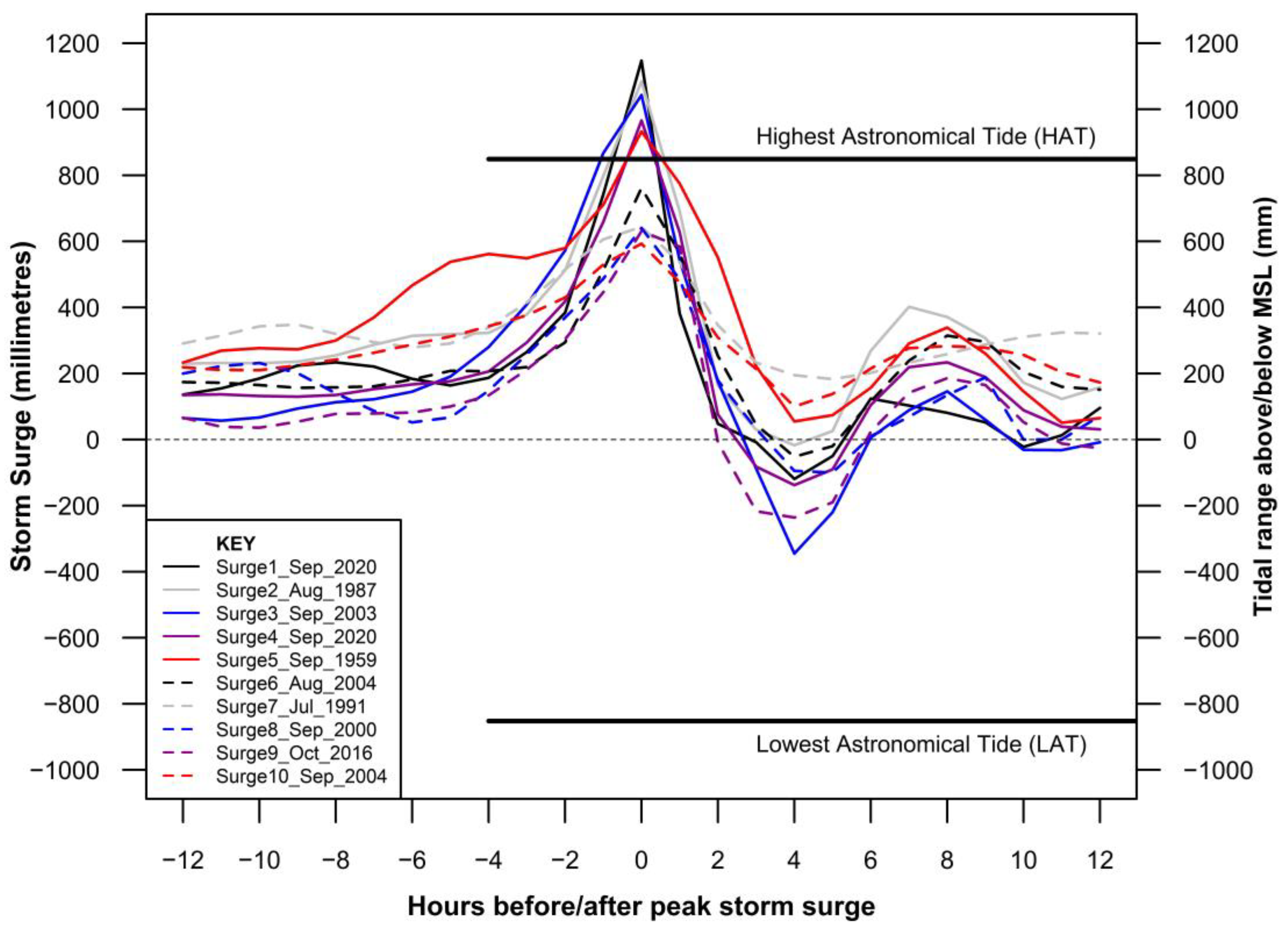
Water levels are maximized when the maximum storm surge coincides with the peak of the tide and, more particularly, during spring tide conditions. Figure 12 highlights the 10 largest storm surge events experienced at Busan as simulated by the Korea Operational Oceanographic System (KOOS) [49] and made available for this study by the Korea Institute of Ocean Science and Technology (KIOST).
There are several key observations evident from this analysis. Firstly, from the 10 highest surge model simulations, it is evident that, for the majority of the events depicted, the peak of the surge rises and falls quite sharply within a couple of hours, which is a characteristic feature essentially governed by the speed of movement of the typhoon system.
The 10 highest surges simulated are all above 590 mm with the largest occurring during the super-typhoon “Haishen” on 3 September 2020 (1147 mm). During this event, the peak of the surge at the tide gauge coincided with a prevailing tide that was falling, significantly limiting the actual height that could have been reached if the peak surge arrived on the preceding high tide.
The extreme water level above the MSL recorded during “Haishen” ranked 6th highest overall (1071 mm; refer to Table 1) but occurred some 5 h earlier with tidal conditions close to the HAT, when the simulated storm surge was only 164 mm.
By contrast, the 3rd highest storm surge (1043 mm) at Busan, which occurred during the super-typhoon “Maemi” on 12 September 2003, occurred close to the peak of the high tide that evening, producing the highest extreme SWL above the MSL on the historical record. Although the extreme SWL above the MSL for the “Maemi” event overshadows the whole record at Busan, it is sobering to consider that the peak tide on the day “Maemi” impacted the Korean Peninsula was substantially lower than HAT. Based on the analysis of these two key events on the tide gauge records at Busan, it is highly improbable from the available records that the peak storm surge driven by a super-typhoon event coincided with the peak of a high spring tide at this location. Such a combination of coincident, yet unrelated factors is merely a matter of chance at some future point. Should such factors align, it would not be physically improbable for extreme SWLs above the MSL to approach 500 mm higher than that reached during the extraordinary super-typhoon “Maemi” event.
Dangendorf et al. (2016) [50] provided a similar discussion concerning the influence of the exceptional storm event “Xaver”, which broke SWL records around the southeastern North Sea in December 2013. A conventional EVA following “Xaver” significantly increased design water levels and this event produced record high water levels. However, Dangendorf et al. (2016) [50] observed that not all key physical components (e.g., tides and surges) were synchronized during the event to result in an observational maximum.
Whist “Xaver” redefined EVA design water levels for the southeastern North Sea, like “Maemi” for Busan and the southern coasts of Korea, neither produced a “theoretical” maximum worst-case scenario due to the coincidence of peak storm surges with lower than exceptional tides.
4.5. Some Thoughts on the Best Practice EVA for Application to Ocean SWLs
Guidance on the best practice application of EVA for deriving design ocean SWLs from long tide gauge records has been significantly advanced in the scientific literature over the past decade [17,19].
On the one hand, it can be rationally argued that the consideration of lengthy, hourly tide gauge records provides an exceptional basis for EVA as all oceanographic and physical phenomena affecting ocean SWLs are automatically recorded at the tide gauge and therefore intrinsically incorporated within the analysis.
However, the analysis in Dangendorf et al. (2016) [50] and this study (refer to Section 4.4) demonstrate that the several defining coastal events that significantly revised design ocean SWLs in different regions of the world did not produce a worst-case scenario water level event because of the coincidence of the respective storm surges with less than exceptional tidal conditions.
In most circumstances, extreme ocean water levels will be driven by a combination of meteorologically driven storm surges (e.g., typhoons, hurricanes, tropical cyclones, and extratropical cyclones) coinciding with the prevailing tidal conditions. Both the surge and tidal components are completely independent of each other, coinciding randomly at any given time and location.
An alternative approach for design and risk management purposes might consider the “theoretical” water level attained by assuming that the peak of each respective storm surge event could coincide with the peak predicted tide occurring within each of the respective typhoon, hurricane, tropical cyclone, and extratropical cyclone seasons. This would provide a “theoretical” upper limit of the water level for each of the respective surge producing events, enabling an applied EVA to generate upper-bound (or limit state) return level plots specific to the locations of interest. Such an analysis would likely provide more rigorous, robust EVA predictions for design purposes that minimize risks associated with under designing against “worst-case” scenarios. These suggestions are worthy of more rigorous analytical examination and discussion amongst scientific, statistical, and coastal engineering fraternities.
5. Conclusions
The hourly measured SWLs at the Busan tide gauge from July 1960 provide an excellent dataset for the consideration of the sea level rise and high-frequency extreme water levels for South Korea’s second most populous city and one of the world’s key port facilities.
The highest hourly water level measurement above the MSL (1403 mm) at Busan occurred on 12 September 2003 (2100 h) resulting from the super-typhoon “Maemi”-driven storm surges. The recorded water level (above the MSL) was estimated (from this study) to have a recurrence interval ≈98 years. This category 5 super-typhoon event has been the most destructive to make landfall on the Korean Peninsula since record keeping begun in 1904, breaking numerous records in the process. The dominance of “Maemi” on the historical record is exemplified by the fact that the second highest extreme SWL above the MSL recorded at Busan occurred during the typhoon “Carmen” event in 1960, estimated to occur with a recurrence interval of only 16 years.
This paper provided a state-of-the-art EVA applied to long hourly SWLs recorded at the Busan tidal facility. The statistical recurrence interval for extreme SWLs above the MSL at Busan is summarized in Table 2. When integrated with IPCC (AR6) MSL projections (Table 3), the proposed design SWLs provide improved and updated information for strategic coastal planning, climate change adaptation purposes, and coastal engineering design at Busan, South Korea.
Several additional points of interest arise from the analysis in this paper. Firstly, it was demonstrated that the early part of the available record at the Busan tidal facility (prior to 1962) might not be reliable. The very high initial annual average reading for 1961 is not synchronized with any strong ENSO phasing (e.g., La Niña, El Niño), which would ordinarily be the case for strong departures above/below the MSL trend over time. The reason for the apparent anomaly in these early measurements is unknown and was beyond the focus of this study. Although there is a difference between the modelled return level plots for all data and post-1961 data scenarios, the respective EVA model differences are comparatively small and unlikely to affect the utility of results (refer to Section 3.1 and Section 4.1).
Secondly, although the linear regression analysis suggests a small increase in the height of de-trended extremes above the HAT over the period from 1960 to present (<0.1 mm/y), the associated error margins suggest this slight increase in the slope is not statistically significant nor different to zero (refer to Section 3.1).
Thirdly, and perhaps most importantly, the random timing of extreme typhoon-driven storm surges and the prevailing tidal conditions are the primary physical processes super-elevating ocean water levels above the MSL at any given point in time. Despite the influences of the super-typhoons “Maemi” (2003) and “Haishen” (2020) on the extreme measured water levels at Busan, the coincident tides at the peak of the storm surges generated were both less than exceptional. This raises the prospect of much greater extremes in future than have been measured to date, owing to the random timing of the “worst-case” conditions during typhoon season (refer to Section 4.4 and Section 4.5).
This work is intended to be expanded to encompass other long tide gauge records stationed around the Korean Peninsula (Incheon, Mokpo, Mukho, Ulsan, Yeosu, and Jeju) in the future.
Author Contributions
Conceptualization, P.J.W. and H.-S.L.; methodology, P.J.W.; software, P.J.W.; formal analysis, P.J.W.; data curation, P.J.W. and H.-S.L.; writing—original draft preparation, P.J.W.; review and editing, H.-S.L. and P.J.W.; supervision, H.-S.L.; project administration, H.-S.L.; funding acquisition, H.-S.L. All authors have read and agreed to the published version of the manuscript.
Funding
This research was supported by the Korea Institute of Marine Science & Technology Promotion (KIMST), funded by the Ministry of Oceans and Fisheries, Republic of Korea (RS-2023-00256687).
Data Availability Statement
Datasets are available upon request from the corresponding author.
Conflicts of Interest
The authors declare no conflict of interest. The funders had no role in the design of the study; in the collection, analyses, or interpretation of data; in the writing of the manuscript; or in the decision to publish the results.
References
- World Population Review. Available online: https://worldpopulationreview.com/countries/cities/south-korea (accessed on 6 September 2023).
- World Shipping Council. Available online: https://www.worldshipping.org/top-50-ports (accessed on 6 September 2023).
- Kim, J.-M.; Son, K.; Yum, S.-G.; Ahn, S.; Ferreira, T. Typhoon Vulnerability Analysis in South Korea Utilizing Damage Record of Typhoon Maemi. Adv. Civ. Eng. 2020, 2020, 8885916. [Google Scholar] [CrossRef]
- Lin, I.-I.; Wu, C.-C.; Emanuel, K.A.; Lee, I.-H.; Wu, C.-R.; Pun, I.-F. The Interaction of Supertyphoon Maemi (2003) with a Warm Ocean Eddy. Mon. Weather. Rev. 2005, 133, 2635–2649. [Google Scholar] [CrossRef]
- Lim, D.-U.; Suh, K.-D.; Mori, N. Regional Projection of Future Extreme Wave Heights around Korean Peninsula. Ocean Sci. J. 2013, 48, 439–453. [Google Scholar] [CrossRef]
- Kim, D.-Y.; Park, S.-H.; Woo, S.-B.; Jeong, K.-Y.; Lee, E.-I. Sea Level Rise and Storm Surge around the Southeastern Coast of Korea. J. Coast. Res. 2017, 79, 239–243. [Google Scholar] [CrossRef]
- Ko, D.H.; Jeong, S.T.; Cho, H. Statistical Characteristics of Hourly Tidal Levels around the Korean Peninsula. J. Korean Soc. Coast. Ocean Eng. 2013, 25, 365–373. [Google Scholar] [CrossRef]
- Byun, D.S.; Choi, B.J.; Kim, H. Estimation of the Lowest and Highest Astronomical Tides along the West and South Coast of Korea from 1999 to 2017. Sea J. Korean Soc. Oceanogr. 2019, 24, 495–508. [Google Scholar] [CrossRef]
- Watson, P.J.; Lim, H.S. An Update on the Status of Mean Sea Level Rise around the Korean Peninsula. Atmosphere 2020, 11, 1153. [Google Scholar] [CrossRef]
- Fox-Kemper, B.; Hewitt, H.T.; Xiao, C.; Aðalgeirsdóttir, G.; Drijfhout, S.S.; Edwards, T.L.; Golledge, N.R.; Hemer, M.; Kopp, R.E.; Krinner, G.; et al. Ocean, Cryosphere and Sea Level Change. In Climate Change 2021: The Physical Science Basis. Contribution of Working Group I to the Sixth Assessment Report of the Intergovernmental Panel on Climate Change; Masson-Delmotte, V., Zhai, P., Pirani, A., Connors, S.L., Péan, C., Berger, S., Caud, N., Chen, Y., Goldfarb, L., Gomis, M.I., et al., Eds.; Cambridge University Press: Cambridge, UK; New York, NY, USA, 2021; pp. 1211–1362. [Google Scholar]
- Rashid, M.M.; Wahl, T. Predictability of Extreme Sea Level Variations Along the U.S. Coastline. J. Geophys. Res. Ocean. 2020, 9, e2020JC016295. [Google Scholar] [CrossRef]
- Arns, A.; Wahl, T.; Haigh, I.D.; Jensen, J. Determining Return Water Levels at Ungauged Coastal Sites: A Case Study for Northern Germany. Ocean Dyn. 2015, 65, 539–554. [Google Scholar] [CrossRef]
- Arns, A.; Wahl, T.; Wolff, C.; Vafeidis, A.T.; Haigh, I.D.; Woodworth, P.; Niehüser, S.; Jensen, J. Non-Linear Interaction Modulates Global Extreme Sea Levels, Coastal Flood Exposure, and Impacts. Nat. Commun. 2020, 11, 1918. [Google Scholar] [CrossRef]
- Schindelegger, M.; Green, J.A.M.; Wilmes, S.-B.; Haigh, I.D. Can We Model the Effect of Observed Sea Level Rise on Tides? J. Geophys. Res. Ocean. 2018, 123, 4593–4609. [Google Scholar] [CrossRef]
- Coles, S. An Introduction to Statistical Modeling of Extreme Values; Springer London: London, UK, 2001; ISBN 978-1-84996-874-4. [Google Scholar]
- Dupuis, D.J. Exceedances over High Thresholds: A Guide to Threshold Selection. Extremes 1999, 1, 251–261. [Google Scholar] [CrossRef]
- Arns, A.; Wahl, T.; Haigh, I.D.; Jensen, J.; Pattiaratchi, C. Estimating Extreme Water Level Probabilities: A Comparison of the Direct Methods and Recommendations for Best Practise. Coast. Eng. 2013, 81, 51–66. [Google Scholar] [CrossRef]
- Caires, S. Extreme Value Analysis: Wave Data; (JCOMM Technical Report 57); World Meteorological Organization/JCOMM: Geneva, Switzerland, 2011; 33p. [Google Scholar] [CrossRef]
- Watson, P.J. Extreme Value Analysis of Ocean Still Water Levels along the USA East Coast—Case Study (Key West, Florida). Coasts 2023, 3, 294–312. [Google Scholar] [CrossRef]
- R Development Core Team. R: A Language and Environment for Statistical Computing, Version 4.3.2; R Foundation for Statistical Computing: Vienna, Austria, 2023. Available online: https://www.r-project.org/(accessed on 29 November 2023).
- Gilleland, E.; Katz, R.W. ExtRemes 2.0: An Extreme Value Analysis Package in R. J. Stat. Softw. 2016, 72, 39. [Google Scholar] [CrossRef]
- Garner, G.G.; Kopp, R.E.; Hermans, T.; Slangen, A.B.A.; Edwards, T.L.; Levermann, A.; Nowikci, S.; Palmer, M.D.; Smith, C.; Fox-Kemper, B.; et al. IPCC AR6 Sea-Level Rise Projections, Version 20210809; PO.DAAC: Pasadena, CA, USA, 2021.
- Garner, G.G.; Kopp, R.E.; Hermans, T.; Slangen, A.B.A.; Koubbe, G.; Turilli, M.; Jha, S.; Edwards, T.L.; Levermann, A.; Nowikci, S.; et al. Framework for Assessing Changes To Sea-Level (FACTS). Geosci. Model Dev. 2022. [Google Scholar] [CrossRef]
- Japan Meterological Organisation. Regional Specialized Meteorological Center (RSMC) Tokyo—Typhoon Center. Available online: https://www.jma.go.jp/jma/jma-eng/jma-center/rsmc-hp-pub-eg/trackarchives.html (accessed on 1 June 2023).
- Embrechts, P.; Klüppelberg, C.; Mikosch, T. Modelling Extremal Events; Springer: Berlin/Heidelberg, Germany, 1997; ISBN 978-3-642-08242-9. [Google Scholar]
- Ramachandra Rao, A.; Hamed, K.H. (Eds.) Flood Frequency Analysis; CRC Press: Boca Raton, FL, USA, 2019; ISBN 9780429128813. [Google Scholar]
- Gumbel, E.J. Statistics of Extremes; Columbia University Press: New York, NY, USA, 1958. [Google Scholar] [CrossRef]
- Beirlant, J.; Goegebeur, Y.; Teugels, J.; Segers, J. Statistics of Extremes; John Wiley & Sons, Ltd.: Chichester, UK, 2004; ISBN 9780470012383. [Google Scholar]
- Pickands, J. Statistical Inference Using Extreme Order Statistics. Ann. Stat. 1975, 3, 119–131. [Google Scholar]
- Watson, P.J. Status of Mean Sea Level Rise around the USA (2020). GeoHazards 2021, 2, 80–100. [Google Scholar] [CrossRef]
- Watson, P.J. Identifying the Best Performing Time Series Analytics for Sea Level Research. In Time Series Analysis and Forecasting: Contributions to Statistics; Rojas, I., Pomares, H., Eds.; Springer International Publishing: Berlin/Heidelberg, Germany, 2016; pp. 261–278. [Google Scholar]
- Watson, P.J. Improved Techniques to Estimate Mean Sea Level, Velocity and Acceleration from Long Ocean Water Level Time Series to Augment Sea Level (and Climate Change) Research. Ph.D. Thesis, University of New South Wales, Sydney, Australia, 2018. [Google Scholar]
- Kondrashov, D.; Ghil, M. Spatio-Temporal Filling of Missing Points in Geophysical Data Sets. Nonlinear Process. Geophys. 2006, 13, 151–159. [Google Scholar] [CrossRef]
- Golyandina, N.; Korobeynikov, A.; Zhigljavsky, A. Singular Spectrum Analysis with R; Springer: Berlin/Heidelberg, Germany, 2018; ISBN 9783662573785. [Google Scholar]
- Watson, P.J. TrendSLR: Estimating Trend, Velocity and Acceleration from Sea Level Records, Version 1.0. In Extension Software Package in R; 2019; Available online: https://cran.r-project.org/web/packages/TrendSLR/index.html (accessed on 29 November 2023).
- Houston, J.R.; Dean, R.G. Effects of Sea-Level Decadal Variability on Acceleration and Trend Difference. J. Coast. Res. 2013, 29, 1062–1072. [Google Scholar] [CrossRef]
- Katz, R.W.; Parlange, M.B.; Naveau, P. Statistics of Extremes in Hydrology. Adv. Water Resour. 2002, 25, 1287–1304. [Google Scholar] [CrossRef]
- Watson, P.J. Determining Extreme Still Water Levels for Design and Planning Purposes Incorporating Sea Level Rise: Sydney, Australia. Atmosphere 2022, 13, 95. [Google Scholar] [CrossRef]
- Ghosh, S.; Resnick, S. A Discussion on Mean Excess Plots. Stoch. Process. Their Appl. 2010, 120, 1492–1517. [Google Scholar] [CrossRef]
- Scarrott, C.; MacDonald, A. A Review of Extreme Value Threshold Estimation and Uncertainty Quantification. REVSTAT-Stat. J. 2012, 10, 33–60. [Google Scholar]
- Thompson, P.; Cai, Y.; Reeve, D.; Stander, J. Automated Threshold Selection Methods for Extreme Wave Analysis. Coast. Eng. 2009, 56, 1013–1021. [Google Scholar] [CrossRef]
- Davison, A.C.; Smith, R.L. Models for Exceedances Over High Thresholds. J. R. Stat. Soc. Ser. B (Methodol.) 1990, 52, 393–425. [Google Scholar] [CrossRef]
- Teena, N.V.; Sanil Kumar, V.; Sudheesh, K.; Sajeev, R. Statistical Analysis on Extreme Wave Height. Nat. Hazard. 2012, 64, 223–236. [Google Scholar] [CrossRef]
- Park, D.-S.R.; Ho, C.-H.; Kim, J.-H.; Kim, H.-S. Strong Landfall Typhoons in Korea and Japan in a Recent Decade. J. Geophys. Res. 2011, 116, D07105. [Google Scholar] [CrossRef]
- Wu, M.C.; Chang, W.L.; Leung, W.M. Impacts of El Niño–Southern Oscillation Events on Tropical Cyclone Landfalling Activity in the Western North Pacific. J. Clim. 2004, 17, 1419–1428. [Google Scholar] [CrossRef]
- Kim, J.-H.; Ho, C.-H.; Sui, C.-H.; Park, S.K. Dipole Structure of Interannual Variations in Summertime Tropical Cyclone Activity over East Asia. J. Clim. 2005, 18, 5344–5356. [Google Scholar] [CrossRef]
- Choi, K.-S.; Kim, B.-J. Climatological Characteristics of Tropical Cyclones Making Landfall over the Korean Peninsula. J. Korean Meteorol. Soc. 2007, 43, 97–109. [Google Scholar]
- Hawkes, P.J.; Gonzalez-Marco, D.; Sánchez-Arcilla, A.; Prinos, P. Best Practice for the Estimation of Extremes: A Review. J. Hydraul. Res. 2008, 46, 324–332. [Google Scholar] [CrossRef]
- Park, K.-S.; Heo, K.-Y.; Jun, K.; Kwon, J.-I.; Kim, J.; Choi, J.-Y.; Cho, K.-H.; Choi, B.-J.; Seo, S.-N.; Kim, Y.H.; et al. Development of the Operational Oceanographic System of Korea. Ocean Sci. J. 2015, 50, 353–369. [Google Scholar] [CrossRef]
- Dangendorf, S.; Arns, A.; Pinto, J.G.; Ludwig, P.; Jensen, J. The Exceptional Influence of Storm ‘Xaver’ on Design Water Levels in the German Bight. Environ. Res. Lett. 2016, 11, 054001. [Google Scholar] [CrossRef]
Figure 1.
Location of the Busan tidal facility. The upper figure shows the location of Busan in the Korean Peninsula, whilst the lower figure (inset) provides the precise location of the Busan tidal facility. Lower image map sourced from Google Earth (accessed 23 November 2023).
Figure 1.
Location of the Busan tidal facility. The upper figure shows the location of Busan in the Korean Peninsula, whilst the lower figure (inset) provides the precise location of the Busan tidal facility. Lower image map sourced from Google Earth (accessed 23 November 2023).

Figure 2.
Summary of tide gauge measurements at Busan. The upper panel depicts the annual MSL over the record. The center panel portrays detrended hourly measurements, whilst the bottom panel highlights the 5 largest events on the historical record (above the MSL) from the declustered extreme events exceeding the HAT.
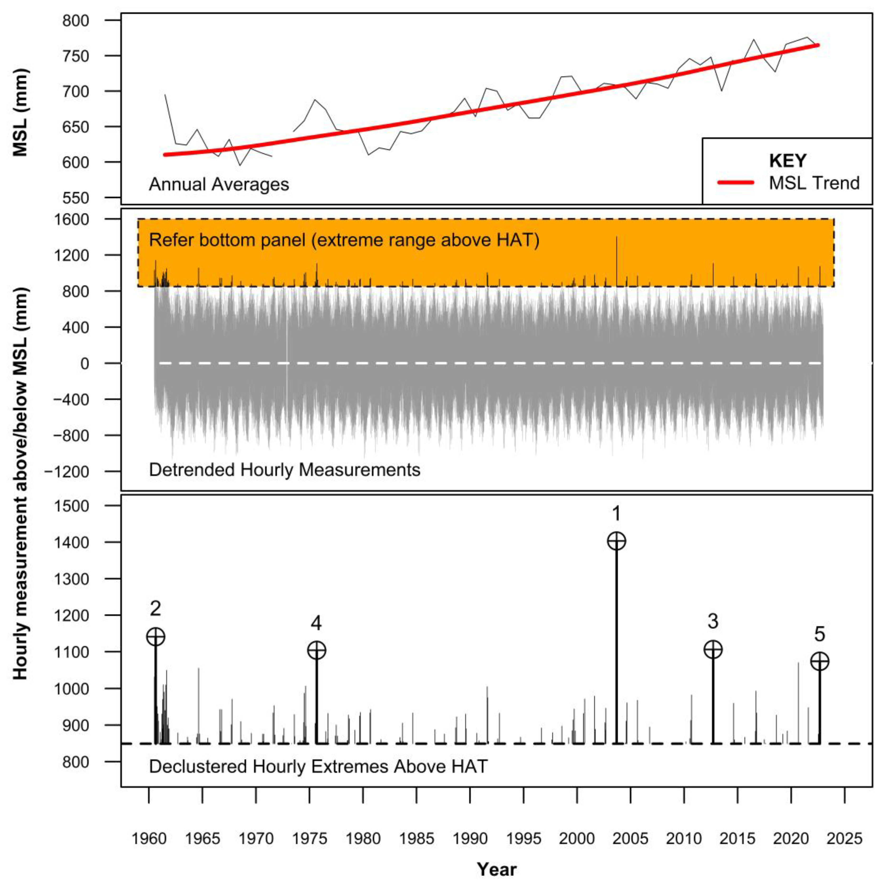
Figure 3.
Typhoon storm tracks that resulted in the largest extreme water level event recorded at Busan. Track data sourced from the Regional Specialized Meteorological Center (RSMC) Tokyo—Typhoon Center [24].
Figure 3.
Typhoon storm tracks that resulted in the largest extreme water level event recorded at Busan. Track data sourced from the Regional Specialized Meteorological Center (RSMC) Tokyo—Typhoon Center [24].

Figure 4.
Linear analysis of the measured extremes above the MSL (>HAT). Data sourced from Figure 2, bottom panel.
Figure 4.
Linear analysis of the measured extremes above the MSL (>HAT). Data sourced from Figure 2, bottom panel.
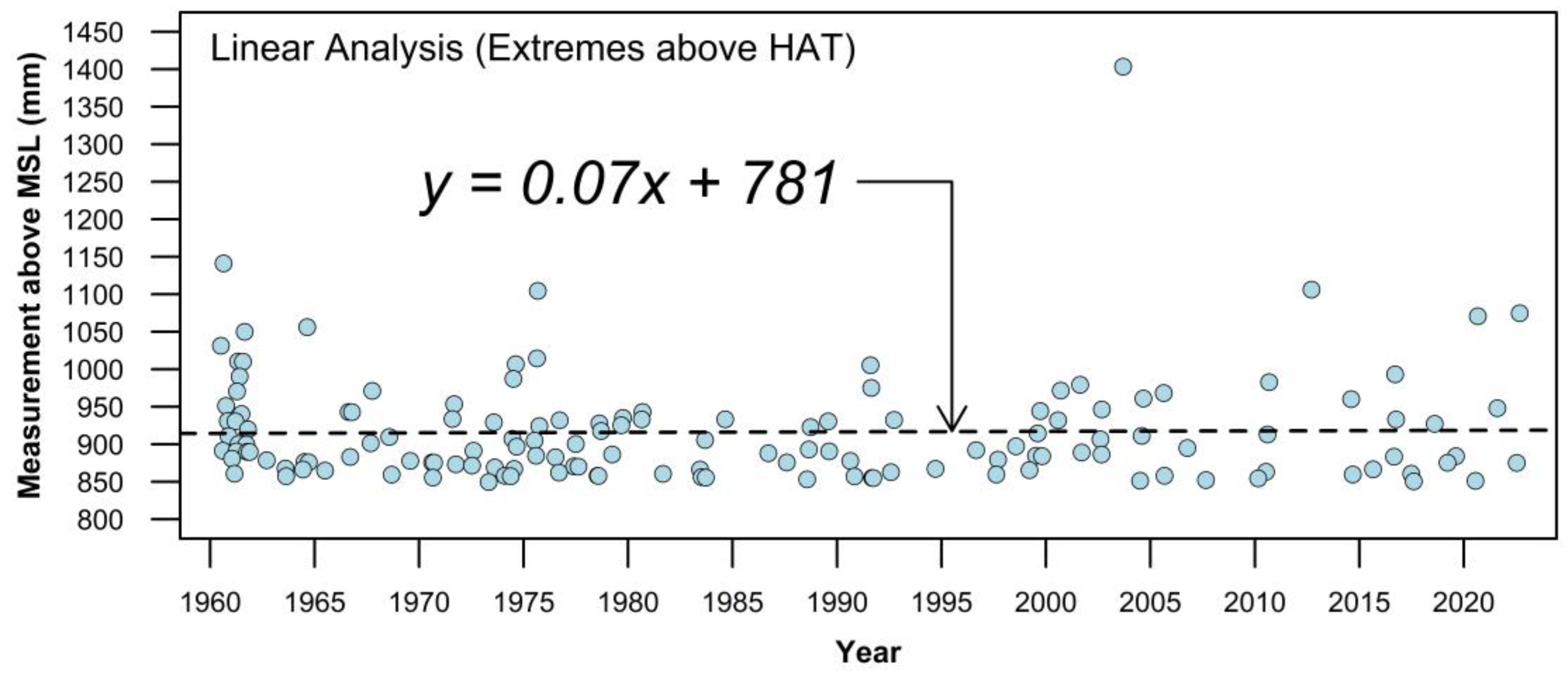
Figure 5.
Mean excess over the threshold plot for Busan. Grey shaded margins represent 95% confidence limits.
Figure 5.
Mean excess over the threshold plot for Busan. Grey shaded margins represent 95% confidence limits.
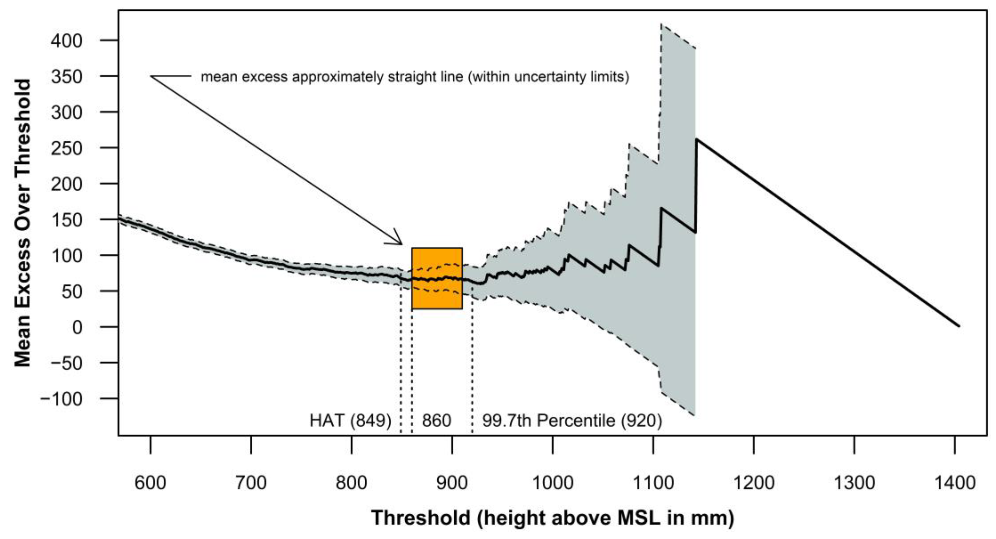
Figure 6.
Sensitivity testing of the threshold selection and parameter estimation method for the EVA at Busan. Thresholds denoted by the MEOT approach (860 mm) and alternative recommended by Arns et al. (2013) [17] are highlighted by dashed vertical lines.
Figure 6.
Sensitivity testing of the threshold selection and parameter estimation method for the EVA at Busan. Thresholds denoted by the MEOT approach (860 mm) and alternative recommended by Arns et al. (2013) [17] are highlighted by dashed vertical lines.
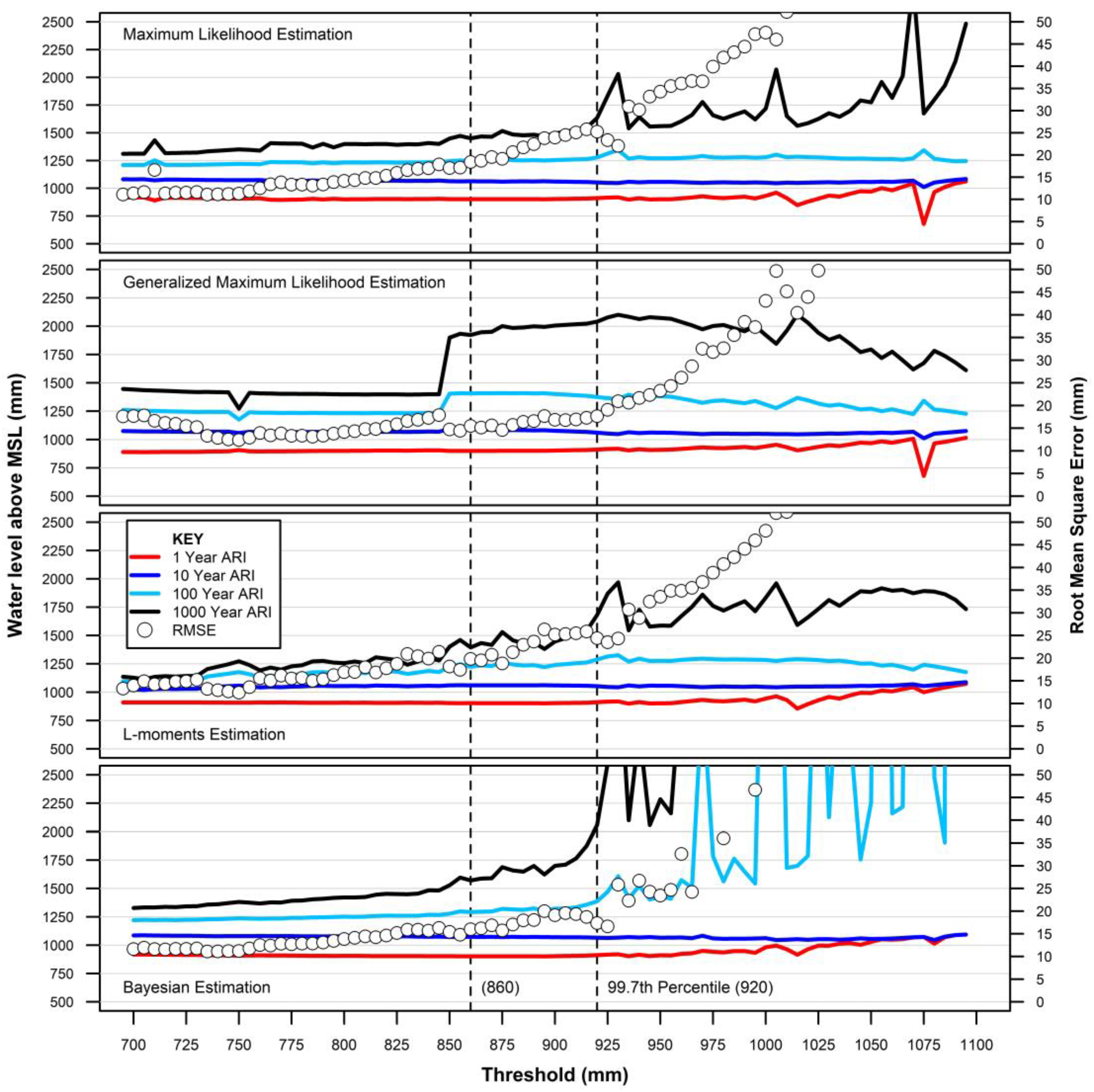
Figure 7.
Recurrence interval plots with the alternative parameter estimation techniques (threshold of 860 mm).
Figure 7.
Recurrence interval plots with the alternative parameter estimation techniques (threshold of 860 mm).
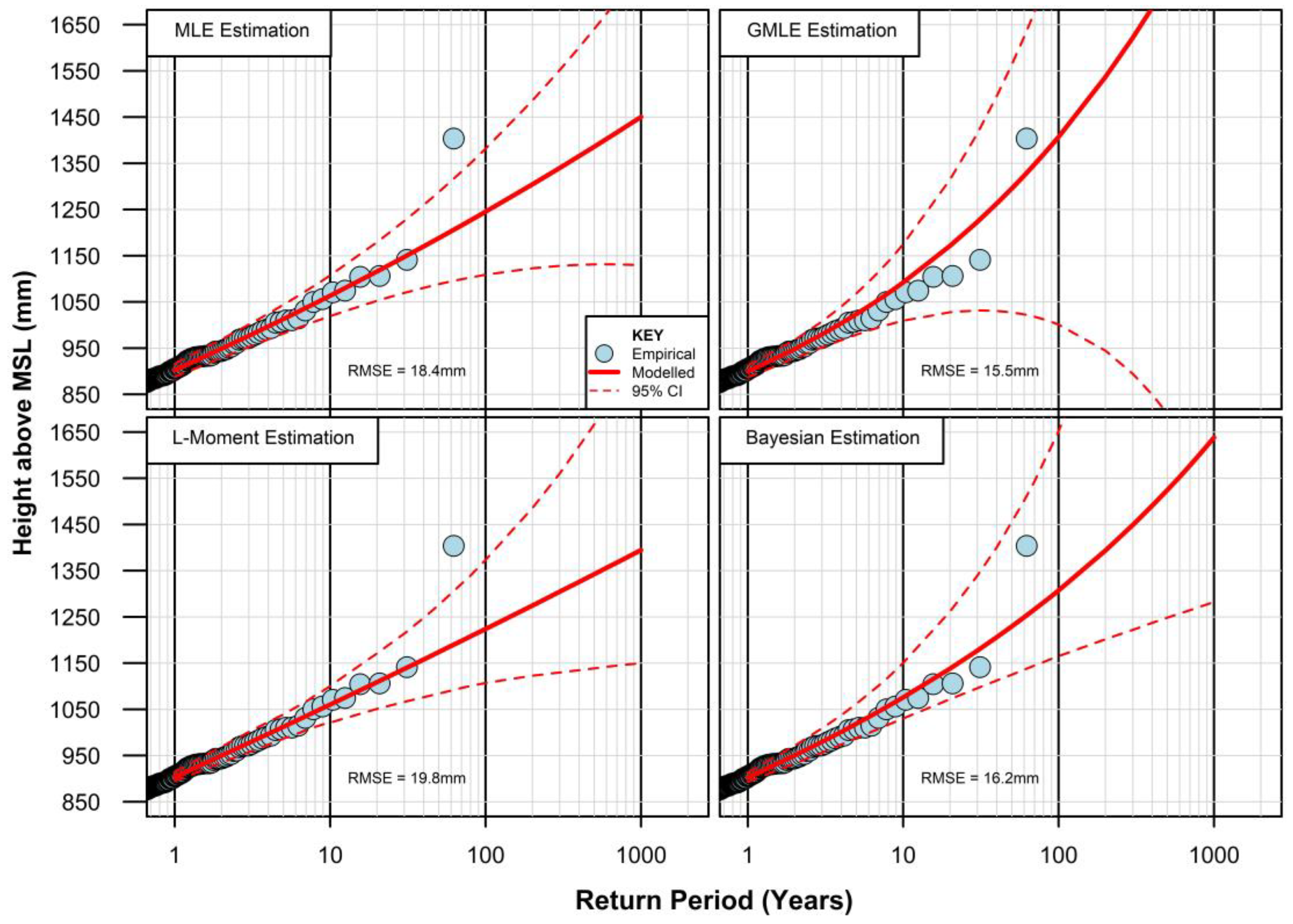
Figure 8.
Sensitivity of the EVA to the early part of the tide gauge record (prior to 1962).

Figure 9.
Impact of the rising mean sea level on the extreme water levels at Busan.
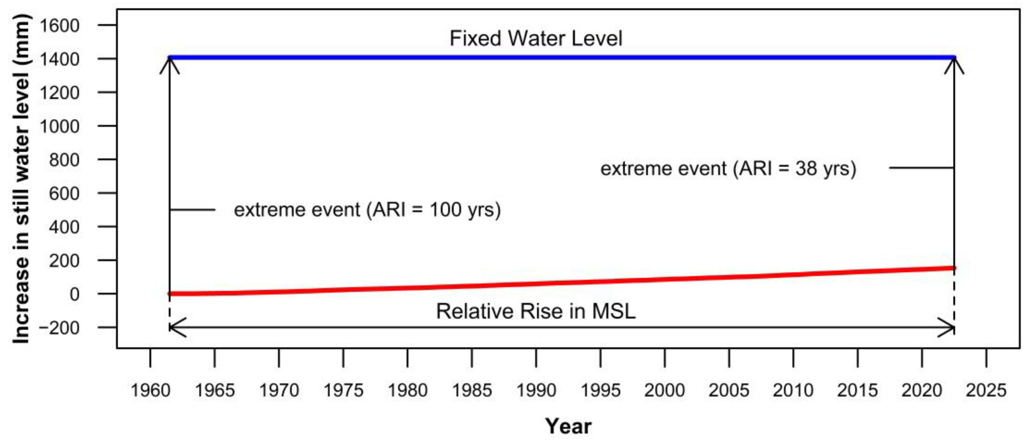
Figure 10.
Influence of the historical and projected increases in the MSLs on the extreme sea levels at Busan using a static water level example.
Figure 10.
Influence of the historical and projected increases in the MSLs on the extreme sea levels at Busan using a static water level example.
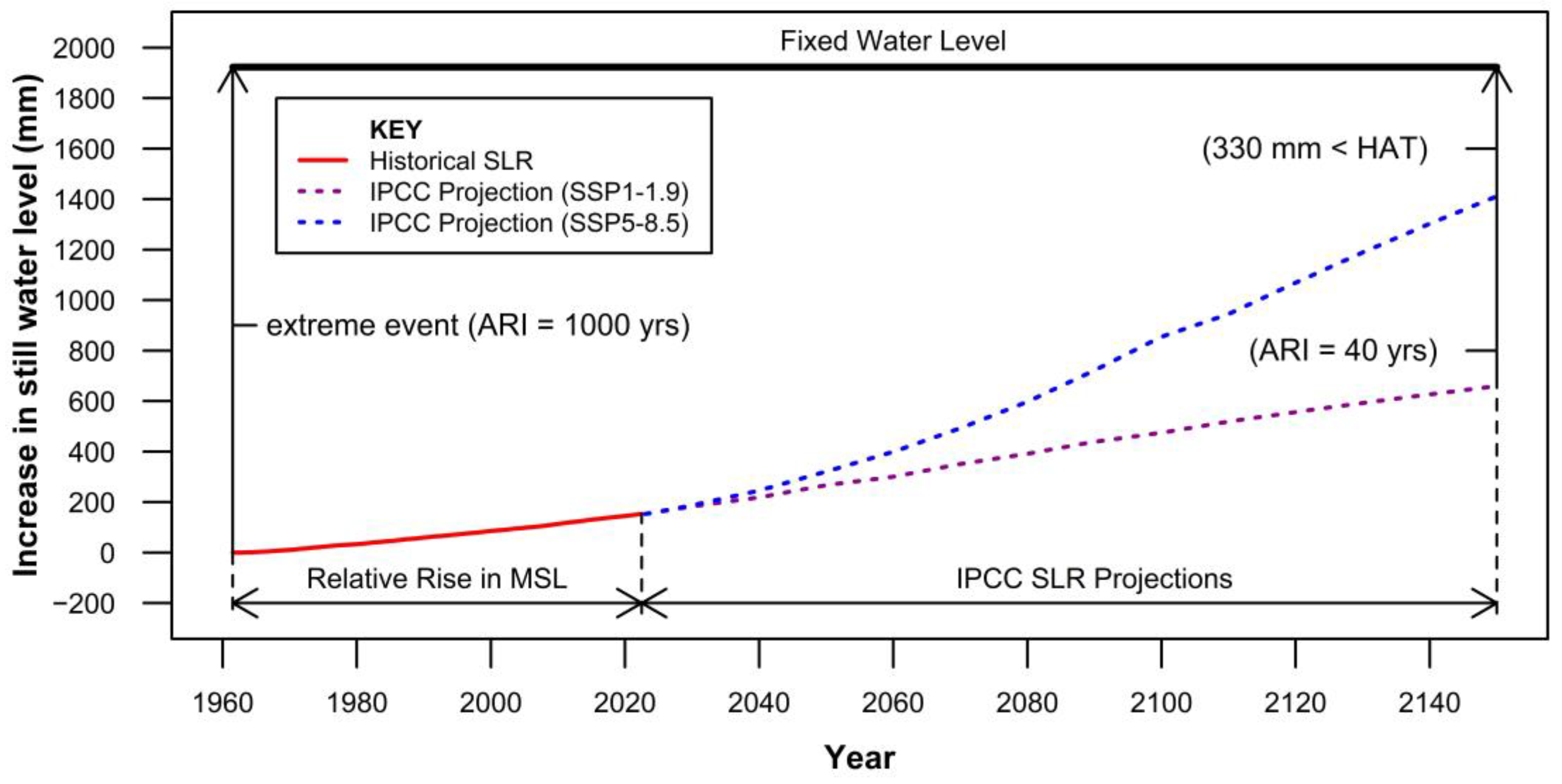
Figure 11.
EVA return period plots for extreme SWLs at Busan both with and without the super-typhoon “Maemi” event.
Figure 11.
EVA return period plots for extreme SWLs at Busan both with and without the super-typhoon “Maemi” event.
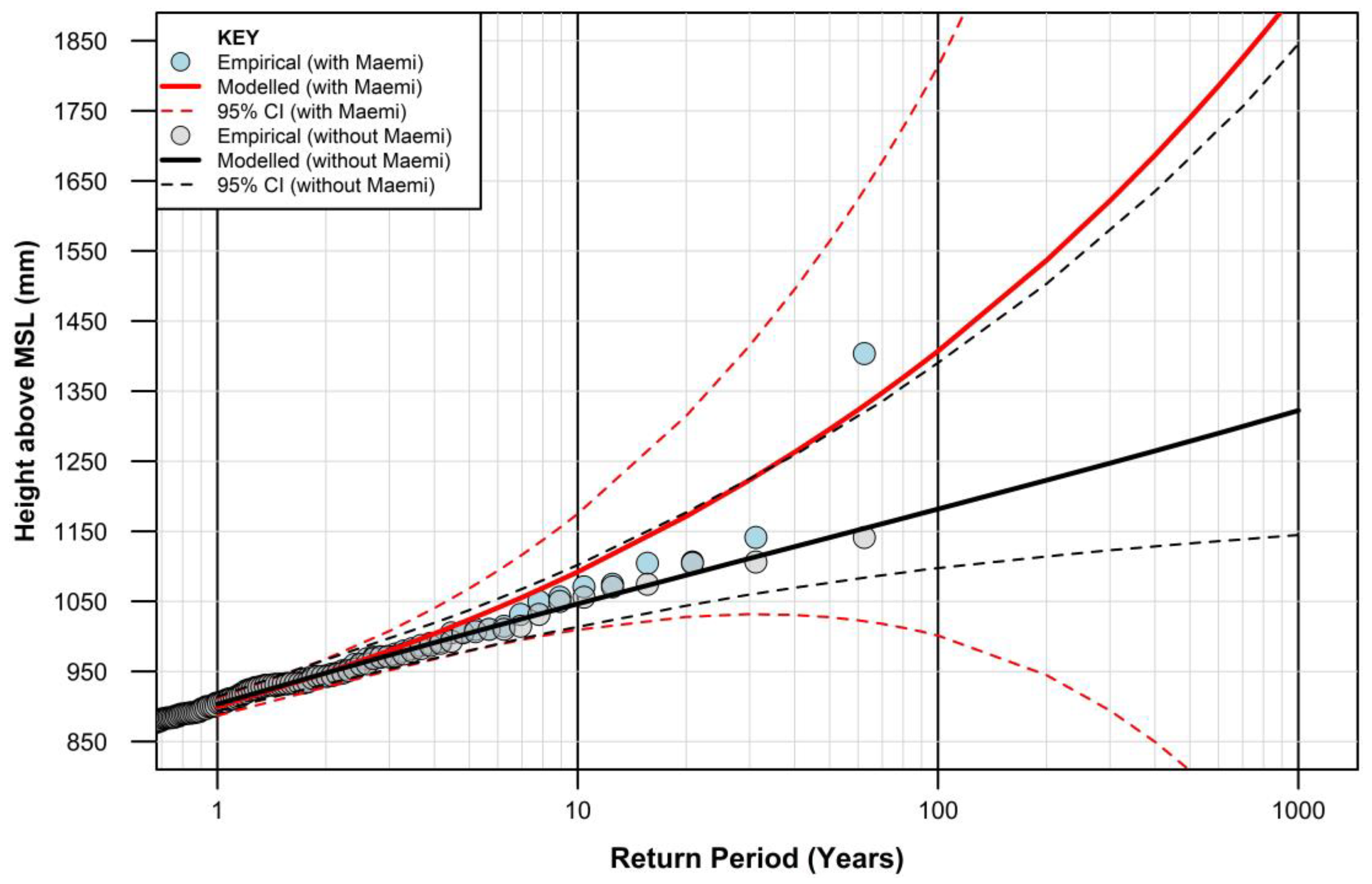
Figure 12.
Top 10 storm surge events at Busan. Surge data from KOOS [49] model simulations made available by KIOST. HAT/LAT provided by Byun et al. (2019) [8].

Table 1.
Highest recorded water levels above the MSL at Busan.
| Rank | Height above MSL (mm) 1 | Date (Time, h) | Typhoon 2 |
|---|---|---|---|
| 1 | 1403 | 12 September 2003 (21:00) | Maemi |
| 2 | 1141 | 22 August 1960 (20:00) | Carmen |
| 3 | 1106 | 17 September 2012 (10:00) | Sanba |
| 4 | 1104 | 6 September 1975 (21:00) | Unknown |
| 5 | 1074 | 6 September 2022 (05:00) | Hinnamnor |
| 6 | 1071 | 2 September 2020 (21:00) | Haishen |
| 7 | 1056 | 23 August 1964 (21:00) | Kathy |
| 8 | 1050 | 27 August 1961 (21:00) | Unknown |
| 9 | 1031 | 8 July 1960 (20:00) | Nadine |
| 10 | 1014 | 23 September 1975 (07:00) | Unknown |
1 Declustered and detrended hourly results. 2 Typhoon event details sourced from the Regional Specialized Meteorological Center (RSMC) Tokyo—Typhoon Center [24].
Table 2.
Summary of the hourly SWLs above the MSL for various recurrence intervals (Busan, South Korea).
Table 2.
Summary of the hourly SWLs above the MSL for various recurrence intervals (Busan, South Korea).
| Recurrence Interval (Years) | Elevation above the MSL (mm) |
|---|---|
| 1 | 900 |
| 2 | 948 |
| 5 | 1024 |
| 10 | 1092 |
| 20 | 1171 |
| 50 | 1296 |
| 100 | 1407 |
| 200 | 1537 |
| 500 | 1740 |
| 1000 | 1923 |
Central model predictions based on Figure 7 (upper right-hand panel).
Table 3.
IPCC AR6 global-averaged sea level projections from 2023 to 2150 (in mm).
| Year | SSP1-1.9 | SSP1-2.6 | SSP2-4.5 | SSP3-7.0 | SSP5-8.5 |
|---|---|---|---|---|---|
| 2023 | 0 | 0 | 0 | 0 | 0 |
| 2030 | 30 | 30 | 31 | 32 | 34 |
| 2040 | 66 | 74 | 80 | 83 | 93 |
| 2050 | 114 | 127 | 142 | 153 | 168 |
| 2060 | 148 | 170 | 200 | 220 | 246 |
| 2070 | 198 | 228 | 268 | 304 | 340 |
| 2080 | 239 | 276 | 341 | 396 | 445 |
| 2090 | 286 | 324 | 414 | 499 | 569 |
| 2100 | 322 | 374 | 494 | 617 | 702 |
| 2110 | 366 | 435 | 566 | 696 | 792 |
| 2120 | 404 | 483 | 640 | 806 | 916 |
| 2130 | 440 | 529 | 713 | 916 | 1036 |
| 2140 | 474 | 575 | 786 | 1024 | 1150 |
| 2150 | 507 | 619 | 857 | 1128 | 1258 |
Disclaimer/Publisher’s Note: The statements, opinions and data contained in all publications are solely those of the individual author(s) and contributor(s) and not of MDPI and/or the editor(s). MDPI and/or the editor(s) disclaim responsibility for any injury to people or property resulting from any ideas, methods, instructions or products referred to in the content. |
© 2023 by the authors. Licensee MDPI, Basel, Switzerland. This article is an open access article distributed under the terms and conditions of the Creative Commons Attribution (CC BY) license (https://creativecommons.org/licenses/by/4.0/).
Share and Cite
MDPI and ACS Style
Watson, P.J.; Lim, H.-S. Extreme Value Analysis of Tide Gauge Record at the Port of Busan, South Korea. GeoHazards 2023, 4, 497-514. https://doi.org/10.3390/geohazards4040028
AMA Style
Watson PJ, Lim H-S. Extreme Value Analysis of Tide Gauge Record at the Port of Busan, South Korea. GeoHazards. 2023; 4(4):497-514. https://doi.org/10.3390/geohazards4040028
Chicago/Turabian StyleWatson, Phil J., and Hak-Soo Lim. 2023. "Extreme Value Analysis of Tide Gauge Record at the Port of Busan, South Korea" GeoHazards 4, no. 4: 497-514. https://doi.org/10.3390/geohazards4040028