
Assessment of Soil Loss from Land Cover Changes in the Nan River Basin, Thailand


International Research Institute of Disaster Science, Tohoku University, Sendai 980-0845, Japan
GeoHazards 2024, 5(1), 1-21; https://doi.org/10.3390/geohazards5010001
Submission received: 20 November 2023
/
Revised: 21 December 2023
/
Accepted: 3 January 2024
/
Published: 4 January 2024
Abstract
:This study investigates soil loss erosion dynamics in the Nan River Basin, Thailand, focusing on the impact of land cover changes. Utilizing the Universal Soil Loss Equation (USLE) model, key factors, including rainfall erosivity, soil erodibility, topography, and land cover, are analyzed for the years 2001 to 2019. The findings reveal a substantial increase in human-induced soil erosion, emphasizing the pressing need for effective mitigation measures. Severity classification demonstrates shifting patterns, prompting targeted conservation strategies. The examination of land cover changes indicates significant alterations in the satellite image (MODIS), particularly an increase in Deciduous forest (~13.21%), Agriculture (~0.18%), and Paddy (~0.43%), and decrease in Evergreen Forest (~13.73%) and Water (~0.12%) cover types. Deciduous forest and Agriculture, associated with the highest soil loss rates, underscore the environmental consequences of specific land use practices. Notably, the increase in Deciduous forest and Agriculture significantly contributes to changes in soil loss rates, revealing the interconnectedness of land cover changes and soil erosion in ~18.05% and ~8.67%, respectively. This study contributes valuable insights for informed land management decisions and lays a foundation for future research in soil erosion dynamics. Additionally, the percentage increase in Agriculture corresponds to a notable rise in soil loss rates, underscoring the urgency for sustainable land use practices.
1. Introduction
In the 21st century, land degradation has become a crucial environmental issue. It is caused by the intricate interplay between climate, geography, and human activities. Soil erosion is the primary consequence of these interactions, which poses a significant threat to land, freshwater, and oceans worldwide. The impacts of this phenomenon are extensive and include a decline in agricultural productivity, ecological harm, and an increase in sedimentation in water bodies. This poses a significant challenge to the sustainability of both water supply and the environment. Therefore, it is essential to implement appropriate measures to mitigate the adverse effects of land degradation and ensure long-term sustainability of the ecosystem [1,2,3,4,5,6,7,8].
The Maritsa Basin is currently facing significant soil erosion, which can be attributed to changes in land use and land cover. This issue has been highlighted by studies that have utilized the Revised Universal Soil Loss Equation (RUSLE) [1]. The impact of soil erosion on food production is a major concern, with an annual loss of 10 million hectares of cropland posing a serious threat to global food security [2]. A study on the Lancang–Mekong River basin, which employed the RUSLE and GIS techniques, has estimated annual soil erosion rates and identified areas that are vulnerable to increased erosion rates and sediment deposition [3]. A comprehensive review of the (R)USLE model has been conducted, which discusses the model’s strengths, limitations, and adaptability to varying conditions. The objective of this review is to improve the model’s global applicability and refine soil loss estimates [4]. Predictions of future water erosion rates indicate the influence of socioeconomic development and climate projections [5]. Another study proposes an extension of the Universal Soil Loss Equation (USLE) to predict nitrogen and phosphorus loss during soil erosion [6]. The USLE and GIS technologies have been utilized in Central Vietnam and Central Chile to assess soil erosion, suggesting targeted solutions and emphasizing the role of vegetative cover in mitigating erosion rates [7,8]. Overall, these studies underscore the importance of understanding and addressing soil erosion for sustainable land use and conservation efforts globally.
Soil loss is mostly attributed to erosion processes, estimated to account for about 84% of global loss [9]. The average rate of soil erosion ranges from 12 to 15 tons per hectare per year [10]. However, it is alarming that human activities cause soil erosion 10–15 times more than natural processes, affecting nearly 80% of cultivated regions worldwide, especially in tropical areas. In these regions, water erosion causes soil loss exceeds 20 tons per hectare per year [11,12]. The excessive sedimentation caused by soil erosion leads to increased turbidity in waterways and high concentrations of impurities, significantly affecting aquatic ecosystems [13].
Understanding the intricate interplay of diverse factors contributing to soil erosion is paramount for devising effective mitigation strategies. Rainfall patterns, topography, soil characteristics, vegetation, land cover changes, cropping systems, and land management practices are among the principal determinants influencing soil erosion rate and severity [14,15]. Accordingly, it becomes crucial to investigate the impact of climate and land cover changes on soil erosion at the regional scale, particularly in watershed areas. Such an investigation would facilitate the development of evidence-based mitigation measures to combat soil erosion.
The assessment of soil erosion has traditionally relied on physically intensive field assessments, which presented significant challenges, including being expensive and impractical for mapping soil erosion risks across large spatial areas with diverse environments [15,16]. Despite these challenges, field-based assessments remain integral to providing accurate data for calibrating and validating soil loss models [6,17,18]. In response to the limitations of field assessments, researchers have made use of various models to map soil loss and erosion risks globally and locally, with the Universal Soil Loss Equation (USLE) and the Revised Universal Soil Loss Equation (RUSLE) emerging as widely used tools [19,20,21].
Various models have been developed to estimate the risks associated with soil loss, utilizing empirical, conceptual, and physical approaches. Such models differ in complexity, data requirements, and calibration processes [22,23]. Empirical models, such as USLE and RUSLE, are particularly beneficial due to their adaptability, minimal data requirements, and broad applicability under diverse conditions [24,25,26,27]. These models are based on observed data and the relationships between factors and soil erosion levels, thus proving advantageous when data availability is limited. However, they often lack detailed information on stream sedimentation deposition, thus constraining their application in modeling mass balance [23].
The primary objective of this paper is to contribute to understanding the impact of land cover changes on soil erosion at the watershed scale. Utilizing the Universal Soil Loss Equation (USLE) method, five highly influential factors were assessed at the pixel level: rainfall, soil type, topography, land cover, and land management. This study focuses on the Upper Nan River Basin in the northern region of Thailand. Specifically, the changes in land cover and their implications for soil erosion between 2001 and 2019 are examined. The ultimate goal is to provide valuable insights to support informed land management and conservation strategies in the region.
2. Materials and Methods
2.1. Study Area
The area upstream of the Nan River Basin holds considerable significance in this study as it plays a vital role in supplying water from the SIRIKIT dam to Thailand’s central region, including the capital city of Bangkok. Figure 1 illustrates the study area in northern Thailand, encompassing a total watershed area of approximately 13,000 km2. The main river originates in the Bor-Klua District, Nan Province, located between latitude 17°42′12″ N and latitude 19°37′48″ N, and longitude 100°06′30″ E to longitude 101°21′48″ E. The topography of the region reveals that a substantial 88% comprises mountainous terrain, with the remaining 12% inhabited by residents within the watershed. Moving downstream from the SIRIKIT dam, which serves as the modeling river outlet, the river bed features a steep slope of approximately 1/1500. As it progresses upstream, the slope transitions to a flat gradient of 1/10,000 before reverting to a steep angle of 1/600. The region has an elevation range of 70 to 1200 m above mean sea level and experiences an average annual rainfall of approximately 1380 mm. The hydrological system in the area is intricate, relying significantly on critical tributaries such as the Wa River, Nam Pua River, and Nam Yao River.
2.2. Rainfall Data
The present study analyzes monthly rainfall data for the basin from 2001 to 2019, provided by the National Aeronautics and Space Administration (NASA) through The Tropical Rainfall Measuring Mission (TRMM) on the 3B43V7 product [28]. Rainfall in this region holds significant importance due to its association with weather patterns originating from the Pacific Ocean and moving westward to the area between March and August. The Inter Tropical Convergence Zone (ITCZ) impacts the northern region of Thailand from May to August, as reported by Schneider et al. [29]. Notably, substantial rainfall between 200 and 450 mm/month was observed during the monsoon event, as depicted in Figure 2a. Figure 2b illustrates the average annual rainfall during the years under consideration, with the maximum value located in the northern area, approximately 1250 mm/year, and the minimum value in the southern region, below 1000 mm/year.
The northern region of Thailand experiences seasonal changes in temperature and monsoon activity. The area is generally hot and humid from November to March, with temperatures ranging from 31 to 38 °C and high relative humidity. The monsoon lows in this area exhibit a cyclonic circulation in the lower troposphere and a warm-cored structure in the upper levels from March to August. The temperature lapse rate in mountainous areas of northern Thailand varies seasonally, with the difference in minimum temperatures changing throughout the year. A combination of wet catchment conditions, heavy rainfall from monsoonal effects or tropical storms, and El Nino Southern Oscillation events cause floods and soil erosion in the region. The temperature and monsoon patterns in the northern area of Thailand are influenced by factors such as the Indian Ocean, the tropical eastern Pacific Ocean, and the high-latitude Asian landmass.
2.3. Soil Data
Thailand’s Land Development Department (LDD) [30] has provided soil data categorized into nine distinct types, as depicted in Figure 3a. The soil in the mountainous regions is primarily composed of sandstone, representing an estimated 83.68% of the total. On the other hand, the surface horizons of soils in floodplain areas contain eight diverse soil types: silty clay, clay loam, sand clay, sandy loam, silty loam, sand clay loam, loam, and clay.
The distribution of organic carbon content in the study area is depicted in Figure 3b. These data were sourced from the United Nations Food and Agriculture Organization (FAO) [31]. The percentage values range from 0 to 3%, with the highest concentration of 3% observed in the wider basin area. Conversely, the floodplain area, located in the middle region, exhibits a comparatively lower value of 1.5%. Notably, the FAO data were instrumental in determining the variability in and distribution of organic carbon content across the study area.
The classification of soil types in the study area is based on the percentage of three main components: sand, silt, and clay. Figure 3c exhibits the percentage distribution of sand in the various soil types across the study area. The border area, which encompasses the mountain region, has the highest concentration of sand, ranging between 90 and 100%. Conversely, the soil of the floodplain region in the middle section has a lower proportion of sand, ranging from 25 to 50%. Figure 3d illustrates the percentage of silt present in the different soil types. The mountain region at the border has a lower silt percentage, at approximately 0–25%. In contrast, the floodplain area has a higher silt percentage, ranging between 50 and 75%. As shown in Figure 3e, the percentage of clay is higher in the middle section of the study area, at approximately 50–100%, and lower in the mountain region at the border, at approximately 0–25%.
2.4. Topography Data
The data used in this study for topography were graciously provided by the United States Geological Survey (USGS), explicitly sourced from the Shuttle Radar Topography Mission (SRTM) [32]. The SRTM project was a joint venture between the National Imagery and Mapping Agency (NIMA) and the National Aeronautics and Space Administration (NASA). The SRTM data are available online through the Consultative Group for International Agriculture Research Consortium for Spatial Information (CGIAR-CSI). The Digital Elevation Model (DEM) data cover approximately 80% of the Earth’s surface, ranging from a latitude of 60 degrees in the north to 60 degrees in the south. The resolution of the data is one arc second, equivalent to approximately 30 m, and boasts 16 m vertical accuracy and 20 m horizontal accuracy at 90% confidence, according to Javis et al. [32]. The original SRTM data were upscaled to 15 × 15 arc-seconds. This pixel size represents a watershed area of 13,000 km2, depicted in Figure 4a, and comprises 457 rows and 292 columns.
Figure 4a shows the digital elevation model (DEM) of the study area, while Figure 4b shows the slope based on the DEM. The mountainous region is situated on a steep slope of approximately 5–30 degrees, whereas the floodplain is characterized by a flat slope of approximately 0–5 degrees. The flow direction data were derived from the slope of the DEM, which facilitated the determination of the downstream direction based on the eight surrounding directions, as illustrated in Figure 4c. Subsequently, flow accumulation data were computed from the flow direction data, representing the number of upstream areas for a given point in the form of grid cells, as displayed in Figure 4d. The Pysheds [33] library created the slope, flow direction, and flow accumulation on the Python 3.8 [34] system.
2.5. Land Cover Data
To acquire land cover data in the study area, data obtained from the Moderate Resolution Imaging Spectroradiometer (MODIS) with a spatial resolution ranging from 250 m to 1 km were utilized. The MODIS data provided the possibility of time series coverage at a moderate resolution. A diverse range of MODIS data in global products, including land cover, primary production, and leaf area index, were used. The MODIS land cover products are primarily available sets of global MODIS products. The product is established from various MODIS-provided inputs such as surface reflectance, vegetation index, surface temperature, and texture. Generated data are provided as a global product according to the worldwide IGBP (International Geosphere–Biosphere Program) classification system [35]. Global MODIS land cover products are suitable for global and regional scales. However, MODIS surface reflectance provided at 250 and 500 m can map regional land cover at a higher resolution according to a user-specified classification system. Empirical analyses have demonstrated that higher resolutions than 1 km are highly desirable for mapping land cover, and the MODIS instrument was designed to deliver 250 and 500 m resolution data.
MCD12Q1 is one of the global MODIS land cover products, of which the data product has been generated annually for twenty years, from 2001 to the present [35]. The MCD12Q1 product of MODIS is obtained by collecting supervised classification samples for each mapping class from 2000 training sites, carried out by the decision tree classifier. The MCD12Q1 product has a global accuracy of approximately 74.8% with a resolution of approximately 500 m. It is categorized into eight classes: Water, Evergreen Forest, Deciduous Forest, Shrub, Agriculture, Paddy, Urban, and Barren. The land cover of the year 2001 is shown in Figure 5a, and the land cover of 2019 is shown in Figure 5b. The difference between both maps reveals a significant change in the area from the Evergreen Forest to Deciduous Forest from the middle to the south. The details of the land cover change for each type are shown in Figure 5c. Water and Evergreen Forests decreased during the years considered, while Deciduous Forests, Shrubland, Agriculture, Paddy, and Barren areas increased. Urban land cover remained unchanged.
2.6. Method of Estimating Soil Loss
The current study utilized the Universal Soil Loss Equation (USLE) model to estimate the potential soil loss risk in the study area. Figure 6 illustrates the applied methodology for this purpose. This study used the Python packages [34] for data analysis and figure generation. The USLE model considers several geospatial factors to calculate the soil loss rate, including rainfall erosivity, soil erodibility, topography, crop management, and conservation practices. Despite its simplicity and suitability for limited data conditions, the model has been widely utilized across the world [22,36,37,38,39,40], including in Ethiopia [41], Kenya [15], Zimbabwe [9], China [26,42,43], Japan [6], India [44,45], Nepal [46,47], Sri Lanka [48], the Philippines [49,50,51], Thailand [52,53], and the Mekong River Basin [3,54,55]. The USLE has also been found to have international applicability and comparability, providing an efficient tool for soil loss estimation and risk assessment. The USLE model [24] is based on an empirical parametric Equation (1), which mathematically estimates the average annual soil loss rate. This equation is expressed as follows:
where is soil loss computed in tons per hectare per year, is the rainfall erosivity factor in megajoules millimeter per hectare per hour per year, is the soil erodibility factor in ton hectare hour hectare−1 mega joule−1 millimater−1, is the topography factor, including with length and steepness of the slope, is the crop management factor, and is the conservation practice factors that are based on the development of an area.
The rainfall erosivity (R-factor) is a crucial metric for gauging the erosive force of rainfall [24]. The erosive power of precipitation depends on the quantity, intensity, and distribution of the rainfall, with intensity being the most significant factor in determining the extent of erosion [56]. To derive the R-factor, satellite rainfall products utilized the TRMM on the 3B43V7 product to obtain monthly data. For rainfall data collection, grid data were accumulated for 19 years, and the annual average factor was used in Equation (2), as provided by Wischmeier [57].
where is the monthly rainfall in millimeters and is the annual rainfall in millimeters.
Soil erodibility (K-factor) is a crucial factor that determines the impact of physical and chemical properties of soil on erosion during storm events in upland areas [20,24]. Soil texture, drainage condition, soil depth, structural integrity, and organic content are some soil properties that can significantly influence soil erodibility [44]. The soil nomograph method is the most commonly used technique for calculating the K-factor. This method determines the K-factor by analyzing the relative ratios of soil texture, permeability, soil structure, and organic matter content [24]. Equation (3) estimates the K-factor, which researchers and practitioners widely use.
where is the percentage of sand content, is the percentage of silt content, is the percentage of clay content, and is the percentage of organic carbon content.
The topographic factor is an essential parameter of the USLE model to determine soil loss. This is because the gravitational force plays a significant role in surface runoff, and the terrain’s topography can significantly impact water flow across its surface [58,59]. The slope length (L) determines the topographic factor, which measures the distance from the source to the top of the intercalation and the slope steepness (S). The LS factor can be calculated using a recommended Equation (4) [60]. Therefore, understanding the topographic factor is critical in predicting and mitigating soil erosion, and it requires careful attention to the relevant parameters and equations.
where is the DEM resolution, m; is the slope of the DEM in percentage; and is the dimensionless exponent of the steepness of the terrain, being 0.5 for the slope > 5%, 0.4 for 3–5%, 0.3 for 1–3%, and 0.2 for <1%.
The crop management factor, also known as the C-factor, is a metric used to determine the extent of soil loss from a specific area subject to a particular cover and management practice. This factor accounts for the protective role of vegetative covers against water erosion [24,61]. In areas lacking vegetation, the soil is highly vulnerable to erosion by water. In contrast, vegetation cover significantly protects the soil surface, reducing erosion. Therefore, increasing vegetation cover can substantially mitigate soil erosion. The C-factor is generally considered the most critical factor in reducing soil erosion. To determine the C-factor, report similar land cover values and compare them with previous studies [4]. In this study, the C-factor was determined based on the land cover type assigned to each area, using values from earlier studies, as illustrated in Table 1.
The conservation practice factor (P-factor) is a critical parameter that quantifies the efficacy of conservation practices in mitigating erosion [24]. The P-factor is a dimensionless value ranging from 0 to 1, with one assigned to areas without erosion control measures [49]. In contrast, areas with adequate protection measures receive a minimum value close to 0. The present study derived the P-factor from the land cover type associated with the C-factor, following the approach recommended by Yang et al. [62]. The values of the P-factor, ascertained from the land cover types, are presented in Table 1 for reference. Notably, the P-factor is an essential parameter that captures the impact of conservation practices on soil loss. By incorporating the P-factor in erosion prediction models, it can better understand the effectiveness of erosion control measures and design efficient strategies to reduce soil erosion.
3. Results
3.1. USLE Factor Estimation Results
Figure 7a illustrates the rainfall erosivity factor (R-factor) ranging from 300 to 500 MJ.mm/ha/h/year, with an average of approximately 400 MJ.mm/ha/h/year. The R-factor distribution was estimated from the monthly Tropical Rainfall Measuring Mission (TRMM) data using the 3B43V7 product over 19 years (2001–2019). The spatial distribution of the R-factor reveals that the northern area exhibited a higher value of approximately 500, whereas the southern area exhibited a lower value of approximately 300. This spatial pattern of the R-factor in the study area corresponds to the annual average rainfall pattern depicted in Figure 2a.
Figure 7b presents the soil erodibility factor (K-factor), which exhibits values ranging from 0 to 0.2 ton.ha.h/ha/MJ/mm, with an average of approximately 0.1 ton.ha.h/ha/MJ/mm. The distribution of the K-factor value was developed from soil data provided by LDD, Thailand, which included nine different soil types in the study area. Notably, the K-factor value distribution is concentrated in the middle of the study area, with a high value of approximately 0.2, mainly in the floodplain area. Conversely, in the mountain area, the K-factor value is low, ranging from approximately 0.05 to 0.1.
The present study examined the LS factor, indicating the topography factor, as illustrated in Figure 7c. The LS-factor values range from 0 to 50, averaging approximately 25. The distribution of the LS factor reveals that the mountainous areas at the border of the study region exhibit high values of approximately 25–50, while the central part has low values of approximately 0–20. The high LS-factor values in the mountainous areas can be attributed to the high steep slope characteristic. Conversely, the low LS-factor values are situated in the floodplain area, characterized by gentle slopes. Notably, the LS factor is a critical parameter in predicting soil erosion caused by water. Therefore, understanding the LS-factor values in different topographical regions is crucial in developing effective erosion control strategies. The present findings provide valuable insights into the topographical features of the study area and contribute to the overall knowledge of soil erosion and its prevention.
Figure 8a,b illustrates the crop management factor (C-factor) for the study area across different land cover categories from 2001 to 2019. The distribution of the C-factor value ranged from 0.001 to 0.5, with high values (0.01 to 0.5) observed in the floodplain area located in the middle of the study area and low values (0.001) in the mountainous border area. Notably, the middle area of the southern part exhibited a significant shift in values between 2001 and 2019, with a significant difference in values between 0.001 and 0.01. This discrepancy can be attributed to alterations in land cover within the study area.
Figure 8c,d showcases the conservation practice factor (P-factor) for 2001 and 2019, respectively. For both the years, the distribution values varied between 0.5 and 1.0. The mountainous area hosts a high value of approximately 1.0, while the middle region contains a low value of around 0.5. These values correspond to the land cover types enumerated in Table 1.
The C-factor and P-factor were identified based on a previous study. It is plausible that the estimation of soil losses in this study may either underestimate or overestimate the actual losses. However, this study employed the change in soil losses to demonstrate the impact of the land cover change. It is important to note that the estimation of soil losses is a complex process that involves several factors, including soil type, slope, and land use. Therefore, the results of this study should be interpreted with caution. Nonetheless, the findings of this study provide valuable insights into the impact of land cover change on soil losses and can be used to inform land management decisions.
3.2. Soil Loss Estimation Result and Its Change between 2001 to 2019
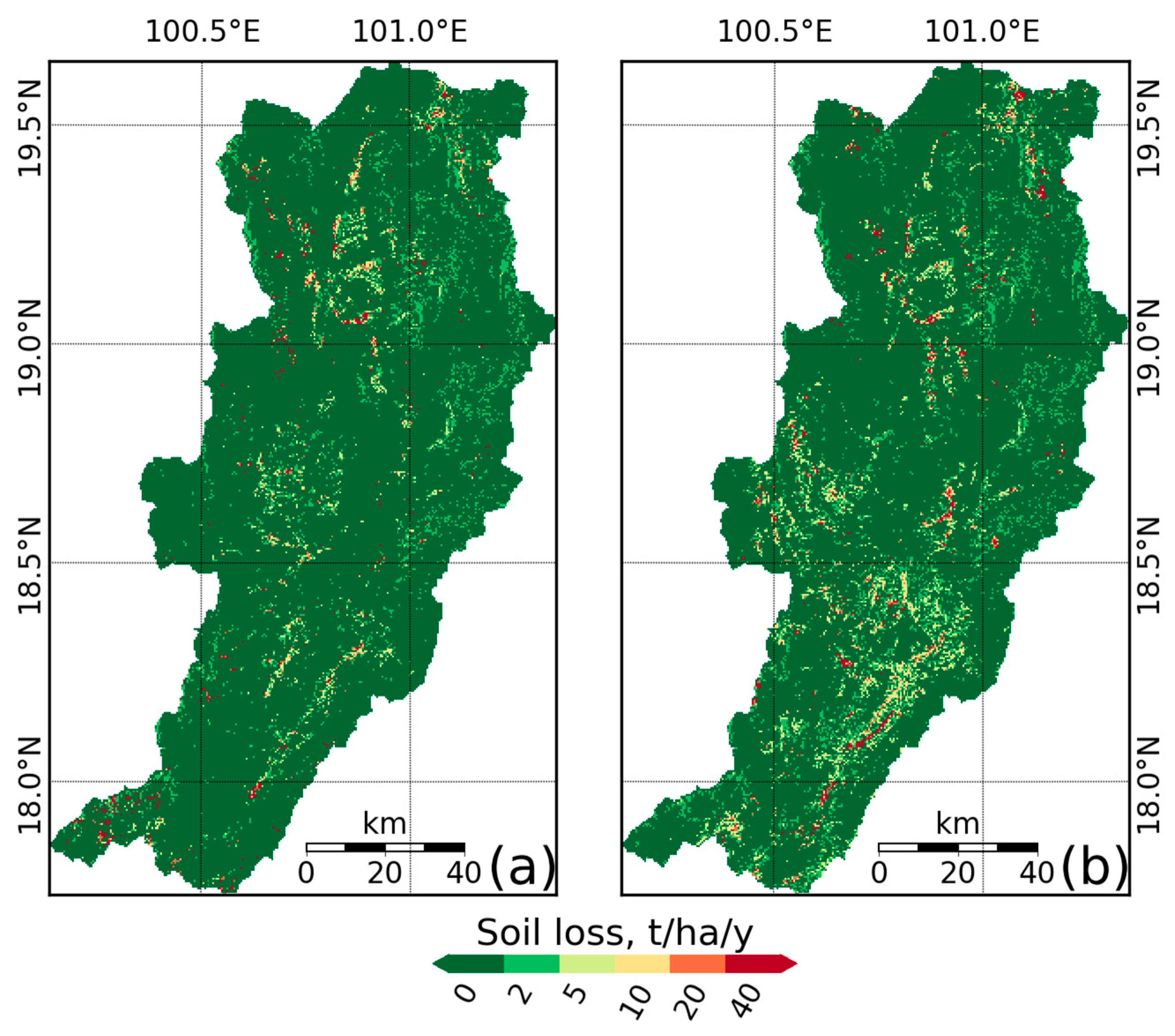
The estimation of soil loss rate relies on five significant factors, as elaborated in the study area information discussed earlier. The distribution of soil loss rate in the study area for 2001 and 2019 is presented in Figure 9a,b, respectively. In 2001, the principal distribution of soil loss rate values was observed over a broad area of approximately 0–2 tons/ha/year. Similarly, in 2019, the primary distribution of soil loss rate values was also approximately 0–2 tons/ha/year. However, there was a considerable difference between the two years in the southern part of the area, with values ranging from 0–2 tons/ha/year to 5–10 tons/ha/year. In 2001, the average range for soil loss rate varied from 0.344 to 132.9 tons/ha/year, while in 2019, it ranged from 0.344 to 125 tons/ha/year.
According to Nut et al. [63] and FAO-PNUMA-UNESCO [64], this study aimed to categorize the soil loss rate into six distinct severity classes. Specifically, the severity classes were very low (0–2 ton/ha/year), low (2–5 ton/ha/year), moderate (5–10 ton/ha/year), severe (10–20 ton/ha/year), very severe (20–40 ton/ha/year), and extremely severe (>40 ton/ha/year). Figure 10a shows the percentage of the area covered by different severity classes in 2001 and 2019. The results indicate that most of the area was classified as very low severity in both years. In 2001, it accounted for 90.90% of the total soil loss, whereas in 2019, it was 85.54%. Conversely, the lowest class was very severe, accounting for 0.46% in 2001 and 0.64% in 2019. Notably, between both years, the percentage of the very low class decreased while the percentage of other classes increased. Furthermore, Figure 10b presents the average soil loss rate difference for each severity class and both years. The extremely severe class had the highest soil loss rate, with approximately 153.34 tons/ha/year in 2001 and 138.51 tons/ha/year in 2019. In contrast, the very low class had the lowest soil loss rate, with approximately 0.39 tons/ha/year in 2001 and 0.44 tons/ha/year in 2019. This study emphasizes the significance of implementing soil conservation practices, particularly in areas with high soil loss rates. Further research is required to identify the causes of soil loss and develop effective strategies to mitigate its impact on the environment and agriculture.
3.3. Soil Loss Estimation Result Relation to Elevation and Slope
The study area was analyzed based on its elevation and corresponding soil loss rate across six different elevation ranges: <300 m, 300–600 m, 600–900 m, 900–1200 m, 1200–1500 m, and above 1500 m [63]. Figure 11a shows the percentage of the area within each elevation range. The highest percentage of the area falls within the 300–600 m range, followed by the 600–900 m range. The lowest percentage of the area is within the less than 300 m and above 1500 m ranges. Figure 11b presents the average soil loss rate for each elevation range in 2001 and 2019. In 2001, the highest average soil loss rate was in the 600–900 m elevation range, with approximately 2.56 tons/ha/year, followed by the 900–1200 m range, with a rate of approximately 2.55 tons/ha/year. The lowest rate was less than 300 m, with approximately 1.53 tons/ha/year. In contrast, in 2019, the highest rate was in the 1200–1500 m range with a rate of approximately 3.41 ton/ha/year, followed by the 900–1200 m range with a rate of approximately 3.23 ton/ha/year. The lowest rate was less than 300 m, with approximately 1.98 tons/ha/year. Overall, all the elevation ranges in 2019 had higher soil loss rates than in 2001.
The slope of the land, estimated using the DEM, was categorized into six different ranges: slopes less than 2 degrees, slopes between 2 and 5 degrees, slopes between 5 and 10 degrees, slopes between 10 and 15 degrees, slopes between 15 and 30 degrees, and slopes greater than 30 degrees [63]. Figure 12a shows the percentage of the area covered by each slope range, with the highest percentage of the area having slopes of less than 2 degrees, covering about 31.02% of the area, followed by slopes between 2 and 5 degrees, covering about 24.02% of the area, and slopes greater than 30 degrees covering the lowest area of about 0.12%. Figure 12b shows the average soil loss rate for each slope range in 2001 and 2019. In 2001, the highest average soil loss rate was observed in slopes greater than 30 degrees, with a rate of approximately 29.85 tons/ha/year, followed by slopes between 15 and 30 degrees, with a rate of approximately 7.47 tons/ha/year, and slopes less than 2 degrees having the lowest rate of approximately 0.49 tons/ha/year. Similarly, in 2019, the highest average soil loss rate was observed in slopes greater than 30 degrees, with a rate of approximately 31.81 tons/ha/year, followed by slopes between 15 and 30 degrees, with a rate of approximately 7.71 tons/ha/year, and slopes less than 2 degrees having the lowest rate of approximately 0.49 tons/ha/year. Overall, the soil loss rate in 2019 was higher than in 2001, except for slopes less than 2 degrees.
3.4. Soil Loss Estimation Result Relation to Land Cover Change and Land Cover Type
The study utilized MODIS land cover data represented by the MCD12Q1 product for the Nan River basin in Thailand between 2001 and 2019. The MCD12Q1 included eight types, namely Water, Evergreen Forest, Deciduous Forest, Shrubland, Agriculture, Paddy, Urban, and Barren. Figure 13a shows each type’s land cover change percentage during this period. The land cover type with the highest decrease is Evergreen Forest at approximately 13.73%, followed by Water at approximately 0.12%. The highest among the increasing land cover types is Deciduous Forest, with approximately 13.21%, followed by Paddy at approximately 0.43%. Deciduous Forests seem to have replaced Evergreen Forests, whereas the other land cover categories changed insignificantly.
Figure 13b presents the soil loss rate related to each land cover type in 2001 and 2019. In 2001, Agriculture had the highest average soil loss at approximately 1929.2 kilotons, followed by Evergreen Forest at approximately 570 kilotons, and Shrubland at approximately 1.7 kilotons as the lowest. In 2019, Agriculture had the highest soil loss at approximately 2170.4 kilotons, followed by Deciduous Forest at approximately 711.1 kilotons, and Barren at approximately 0.4 kilotons as the lowest. Overall, the average soil loss in the Water, Evergreen Forest, Deciduous Forest, Shrubland, Agriculture, Urban, and Barren land cover types were related to the decreasing and increasing land cover change, except for Paddy.
Figure 13c illustrates the total soil loss change percentage for each land cover type from 2001 to 2019. The highest decrease in soil loss was in the Evergreen Forest type at approximately 1.84%, while the highest increase was in Deciduous Forest at approximately 18.05%, followed by Agriculture at approximately 8.67%.
4. Discussions
This study used the Universal Soil Loss Equation (USLE) model to assess the relationship between land cover change and soil erosion in the Nan River Basin in Thailand. The findings reveal several key factors influencing soil loss dynamics in the region. Reference studies [1,2,3,4,5,6,7,8] emphasize the global significance of addressing soil erosion, highlighting its far-reaching consequences on land, freshwater, and ocean ecosystems. The observed spatial variation in rainfall erosivity (R-factor) aligns with prior research [11], emphasizing the critical role of precipitation patterns in influencing soil erosion. Moreover, the concentrated soil erodibility (K-factor) in the floodplain, as indicated by LDD soil data [30], corresponds to previous studies [44], highlighting the influence of soil properties on erosion susceptibility. The LS factor distribution, influenced by topography, underscores the importance of understanding terrain characteristics [58,59] for effective erosion control, particularly in mountainous and floodplain areas.
It is important to understand that research on soil erosion is context-specific, and findings may not be universally applicable. While this study provides valuable insights into the Upper Nan River Basin, its findings should be considered within the specific environmental context studied. A balanced approach that recognizes the strengths and weaknesses of the USLE method will lead to a more nuanced and applicable understanding of soil erosion dynamics.
The comparison of soil loss rates between 2001 and 2019 (Figure 9a,b) echoes concerns raised by global estimates [9,10] regarding the escalating rates of human-induced soil erosion. The distribution of soil loss rate values in both years shows a broad area experiencing low to moderate soil loss (0–2 tons/ha/year), with a significant difference observed in the southern part, where higher values (5–10 tons/ha/year) are evident in 2019. The observed changes in the southern region, with higher soil loss rates in 2019, highlight the need for targeted conservation efforts in response to shifting environmental dynamics. The severity classification (Figure 10a) reveals a nuanced pattern, with a decrease in very low severity and an increase in other classes, indicative of evolving soil erosion challenges. The extremely severe soil loss rates underscore the urgency of implementing effective soil conservation measures [49]. These findings are consistent with studies emphasizing the need for adaptive strategies to mitigate adverse environmental and agricultural impacts [41].
This study presents details on soil erosion in a distinct geographical area. It contrasts the research undertaken in the northwest region of Algeria, which primarily focused on the river basin scale of Wadi Gazouana. Although both studies utilized the Universal Soil Loss Equation (USLE) and its variants, namely the Modified Universal Soil Loss Equation (MUSLE) and the Revised Universal Soil Loss Equation (RUSLE), significant differences emerged in their findings and methodologies. The Algerian study aimed to estimate specific erosion rates in the entire Wadi Ghazouana watershed, given the challenges of water erosion exacerbated by climate change and human intervention [65]. The USLE, RUSLE, and MUSLE models produced erosion rates of 9.65 (t/ha/year), 9.90 (t/ha/year), and 11.33 (t/ha/year), respectively. Of note, the MUSLE model demonstrated a higher spatial dispersion of erosion risk due to the increased effectiveness of the rain factor. These findings offer insights into soil erosion management and mitigation strategies that could be adopted in different regions worldwide.
This study presents an analysis of soil loss rates in a distinct region and highlights a range of erosion rates across severity classes. In particular, the research reveals that the extremely severe class exhibits the highest soil loss rates, with an average of approximately 153.34 tons per hectare per year in 2001 and 138.51 tons per hectare per year in 2019. Conversely, the very low class demonstrates the lowest soil loss rates, averaging around 0.39 tons per hectare per year in 2001 and 0.45 tons per hectare per year in 2019. While both studies offer valuable insights into soil erosion dynamics, the differences in geographic locations, specific methodologies, and the focus on severity classes versus overall erosion rates underscore the complex nature of soil erosion challenges and the importance of customized approaches to address them. The findings highlight the global significance of comprehending and mitigating soil erosion for sustainable land management practices.
The elevation and slope analysis (Figure 11b and Figure 12b) offer insights into topographic influences on soil loss rates. Higher rates in elevated areas and steeper slopes align with established knowledge [58,59], emphasizing the vulnerability of such regions to erosion. This supports the call for targeted conservation strategies in areas characterized by an elevated terrain. Furthermore, the examination of land cover change (Figure 13a) highlights anthropogenic impacts on the landscape. The increase in Deciduous Forest of 13.2% and the corresponding decrease in Evergreen Forest of 13.7% and Water of 0.12% cover types align with concerns raised by environmental studies [44], emphasizing the need for sustainable land management practices. The association of Agriculture with the high average soil loss rates of an approximately 8.67% increase underscores the environmental consequences of specific land use practices [4]. The observed changes in soil loss rates (Figure 13b) and the total soil loss change percentage (Figure 13c) underscore the dynamic nature of soil erosion processes, demanding continuous monitoring and adaptive conservation efforts [3,54,55].
5. Conclusions
The comprehensive analysis sheds light on the intricate dynamics of soil erosion in the Nan River Basin, Thailand, emphasizing the significant impact of land cover changes on soil loss. The study employed the Universal Soil Loss Equation (USLE) model, integrating key factors such as rainfall erosivity, soil erodibility, topography, crop management, and conservation practices to estimate soil loss rates. The results revealed spatial variations in the distribution of factors, with higher rainfall erosivity in the northern region, concentrated soil erodibility in the floodplain, and notable differences in topography influencing the LS factor. The assessment of soil loss rates between 2001 and 2019 uncovered changes, particularly in the southern part of the study area, where higher soil loss rates were evident. The severity classification highlighted the urgency of implementing soil conservation measures, especially in areas experiencing extreme soil loss. Additionally, the elevation, slope, and land cover change analysis provided crucial insights into the topographic and anthropogenic influences on soil erosion susceptibility, emphasizing the need for targeted conservation strategies in elevated and steeper slope regions. These findings contribute valuable information to guide evidence-based land management and conservation strategies in the Nan River Basin, fostering long-term sustainability and resilience against the adverse effects of soil erosion.
Furthermore, the study underscores the interconnected relationship between land cover changes and soil erosion, emphasizing the role of human activities in shaping environmental outcomes. The satellite image (MODIS) showed the increase in Deciduous Forests of 13.2% and the corresponding decrease in Evergreen Forests of 13.7% and Water of 0.13% cover types, highlighting the anthropogenic footprint on the landscape. The average soil loss rates of different land cover types highlight the importance of sustainable land management practices. In areas dominated by Deciduous Forests, the total soil loss increased by 18.05% (501.9 kilotons). The dynamic nature of soil erosion processes, as evidenced by changes in severity classes and soil loss rates over the studied period, emphasizes the need for ongoing monitoring and adaptive conservation measures. Overall, this research provides critical insights into the factors influencing soil erosion in the Nan River Basin and serves as a foundation for informed decision-making, facilitating the development of effective strategies to mitigate soil loss, protect the environment, and promote sustainable land use practices in the region.
Funding
This research received no external funding.
Data Availability Statement
Data are contained within the article.
Acknowledgments
This study used the QGIS 3.28.9 software and Python 3.8.0 to analyze and illustrate the spatial data, including Pysheds 0.3.5.
Conflicts of Interest
The authors declare no conflicts of interest.
References
- Ozsahin, E.; Duru, U.; Eroglu, I. Land Use and Land Cover Changes (LULCC), a key to understand soil erosion intensities in the Maritsa Basin. Water 2018, 10, 335. [Google Scholar] [CrossRef]
- Pimentel, D.; Burgess, M. Soil erosion threatens food production. Agriculture 2013, 3, 443–463. [Google Scholar] [CrossRef]
- Chuenchum, P.; Xu, M.; Tang, W. Estimation of soil erosion and sediment yield in the Lancang–Mekong River using the modified revised universal soil loss equation and GIS techniques. Water 2019, 12, 135. [Google Scholar] [CrossRef]
- Benavidez, R.; Jackson, B.; Maxwell, D.; Norton, K. A review of the (Revised) Universal Soil Loss Equation ((R)USLE): With a view to increasing its global applicability and improving soil loss estimates. Hydrol. Earth Syst. Sci. 2018, 22, 6059–6086. [Google Scholar] [CrossRef]
- Borrelli, P.; Robinson, D.A.; Panagos, P.; Lugato, E.; Yang, J.E.; Alewell, C.; Wuepper, D.; Montanarella, L.; Ballabio, C. Land use and climate change impacts on global soil erosion by water (2015–2070). Proc. Natl. Acad. Sci. USA 2020, 117, 21994–22001. [Google Scholar] [CrossRef] [PubMed]
- Mihara, M.; Yamamoto, N.; Ueno, T. Application of USLE for the prediction of nutrient losses in soil erosion processes. Paddy Water Environ. 2005, 3, 111–119. [Google Scholar] [CrossRef]
- Pham, T.G.; Degener, J.; Kappas, M. Integrated Universal Soil Loss Equation (USLE) and Geographical Information System (GIS) for soil erosion estimation in A Sap Basin: Central Vietnam. Int. Soil Water Conserv. Res. 2018, 6, 99–110. [Google Scholar] [CrossRef]
- Bonilla, C.A.; Reyes, J.L.; Magri, A. Water erosion prediction using the Revised Universal Soil Loss Equation (RUSLE) in a GIS framework, Central Chile. Chil. J. Agric. Res. 2010, 70, 159–169. [Google Scholar] [CrossRef]
- Marondedze, A.K.; Schütt, B. Assessment of soil erosion using the RUSLE model for the Epworth district of the Harare Metropolitan province, Zimbabwe. Sustainability 2020, 12, 8531. [Google Scholar] [CrossRef]
- Ashiagbor, G.; Forkuo, E.K.; Laari, P.; Aabeyir, R. Modeling soil erosion using RUSLE and GIS tools. Int. J. Remote Sens. Geosci. 2013, 2, 17. [Google Scholar]
- Van Oost, K.; Quine, T.A.; Govers, G.; De Gryze, S.; Six, J.; Harden, J.W.; Ritchie, J.C.; McCarty, G.W.; Heckrath, G.; Kosmas, C.; et al. The impact of agricultural soil erosion on the global carbon cycle. Science 2007, 318, 626–629. [Google Scholar] [CrossRef]
- Wilkinson, B.H.; McElroy, B.J. The impact of humans on continental erosion and sedimentation. Geol. Soc. Am. Bull. 2007, 119, 140–156. [Google Scholar] [CrossRef]
- Tang, W.; Shan, B.; Zhang, H.; Zhang, W.; Zhao, Y.; Ding, Y.; Rong, N.; Zhu, X. Heavy metal contamination in the surface sediments of representative limnetic ecosystems in Eastern China. Sci. Rep. 2014, 4, 7152. [Google Scholar] [CrossRef] [PubMed]
- Panagopoulos, Y.; Dimitriou, E.; Skoulikidis, N. Vulnerability of a northeast Mediterranean island to soil loss. Can crazing management mitigate erosion? Water 2019, 11, 1491. [Google Scholar] [CrossRef]
- Kogo, B.K.; Kumar, L.; Koech, R. Impact of land use/cover changes on soil erosion in western Kenya. Sustainability 2020, 12, 9740. [Google Scholar] [CrossRef]
- Chen, T.; Niu, R.; Li, P.; Zhang, L.; Du, B. Regional soil erosion risk mapping using RUSLE, GIS, and remote sensing: A case study in Miyun watershed, north China. Environ. Earth Sci. 2011, 63, 533–541. [Google Scholar] [CrossRef]
- Evans, R. An alternative way to assess water erosion of cultivated land—Field-based measurements and analysis of some results. Appl. Geogr. 2002, 22, 187–207. [Google Scholar] [CrossRef]
- Evans, R.; Brazier, R. Evaluation of modelled spatially distributed predictions of soil erosion by water versus field-based assessments. Environ. Sci. Policy 2005, 8, 493–501. [Google Scholar] [CrossRef]
- Renschler, C.S.; Harbor, J. Soil erosion assessment tools from point to regional scales—The role of geomorphologists in land management research and implementation. Geomorphology 2002, 47, 189–209. [Google Scholar] [CrossRef]
- Renard, K.G.; Foster, G.R.; Weesies, G.A.; McCool, D.K.; Yoder, D.C. Predicting Soil Erosion by Water: A Guide to Conservation Planning with the Revised Universal Soil Loss Equation (RUSLE); Agriculture Handbook No. 703; USDA-ARS: Washington, DC, USA, 1997; p. 404.
- Karydas, C.G.; Panagos, P.; Gitas, I.Z. A classification of water erosion models according to their geospatial characteristics. Int. J. Digit. Earth 2014, 7, 229–250. [Google Scholar] [CrossRef]
- Merritt, W.S.; Letcher, R.A.; Jakeman, A.J. A review of erosion and sediment transport models. Environ. Model. Softw. 2003, 18, 761–799. [Google Scholar] [CrossRef]
- Raza, A.; Ahrends, H.; Habib-Ur-Rahman, M.; Gaiser, T. Modeling approaches to assess soil erosion by water at the field scale with special emphasis on heterogeneity of soils and crops. Land 2021, 10, 422. [Google Scholar] [CrossRef]
- Wischmeier, W.H.; Smith, D.D. Predicting Rainfall Erosion Losses: A Guide to Conservation Planning; Department of Agriculture, Science and Education Administration: Washington, DC, USA, 1978. [Google Scholar]
- Williams, J.R.; Berndt, H.D. Sediment yield prediction based on watershed hydrology. Trans. ASAE 1977, 20, 1100–1104. [Google Scholar] [CrossRef]
- Stefanidis, S.; Alexandridis, V.; Chatzichristaki, C.; Stefanidis, P. Assessing soil loss by water erosion in a typical Mediterranean ecosystem of northern Greece under current and future rainfall erosivity. Water 2021, 13, 2002. [Google Scholar] [CrossRef]
- Alewell, C.; Borrelli, P.; Meusburger, K.; Panagos, P. Using the USLE: Chances, challenges and limitations of Soil erosion modelling. Int. Soil Water Conserv. Res. 2019, 7, 203–225. [Google Scholar] [CrossRef]
- Huffman, G.J.; Adler, R.F.; Bolvin, D.T.; Gu, G.J.; Nelkin, E.J.; Bowman, K.P.; Hong, Y.; Stocker, E.F.; Wolff, D.B. The TRMM multisatellite precipitation analysis (TMPA): Quasi-global, multiyear, combined-sensor precipitation estimates at fine scales. J. Hydrometeorol. 2007, 8, 38–55. [Google Scholar] [CrossRef]
- Schneider, T.; Bischoff, T.; Hang, G.H. Migrations and dynamics of the intertropical convergence zone. Nature 2014, 513, 45–53. [Google Scholar] [CrossRef]
- Land Development Department, Thailand. Soil Type. Available online: https://tswc.ldd.go.th/DownloadGIS/Index_Soil.html (accessed on 1 October 2023).
- FAO Digital Soil Map of the World (DSMW). Available online: https://www.fao.org/land-water/land/land-governance/land-resources-planning-toolbox/category/details/es/c/1026564/ (accessed on 1 October 2023).
- Jarvis, A.; Reuter, H.I.; Nelson, A.; Guevara, E. Hole-Filled SRTM for the Globe Version 4. CGIAR-CSI SRTM 90 m Database 2008. 2012. Available online: http://srtm.csi.cgiar.org (accessed on 1 July 2012).
- Bartos, Pysheds 0.3.5. Available online: https://pypi.org/project/pysheds/ (accessed on 1 October 2023).
- Python 3.8.0. Available online: https://www.python.org/downloads/release/python-380/ (accessed on 1 October 2023).
- Friedl, M.A.; Sulla-Menashe, D.; Tan, B.; Schneider, A.; Ramankutty, N.; Sibley, A.; Huang, X. MODIS Collection 5 global land cover: Algorithm refinements and characterization of new datasets. Remote Sens. Environ. 2010, 114, 168–182. [Google Scholar] [CrossRef]
- Kidane, M.; Bezie, A.; Kesete, N.; Tolessa, T. The impact of Land Use and Land Cover (LULC) dynamics on soil erosion and sediment yield in Ethiopia. Heliyon 2019, 5, e02981. [Google Scholar] [CrossRef]
- Gelagay, H.S.; Minale, A.S. Soil loss estimation using GIS and remote sensing techniques: A case of Koga watershed, northwestern Ethiopia. Int. Soil Water Conserv. Res. 2016, 4, 126–136. [Google Scholar] [CrossRef]
- Tadesse, L.; Suryabhagavan, K.V.; Sridhar, G.; Legesse, G. Land use and land cover changes and soil erosion in Yezat watershed, north western Ethiopia. Int. Soil Water Conserv. Res. 2017, 5, 85–94. [Google Scholar] [CrossRef]
- Balabathina, V.N.; Raju, R.P.; Mulualem, W.; Tadele, G. Estimation of soil loss using remote sensing and GIS-based universal soil loss equation in northern catchment of lake Tana sub-basin, upper Blue Nile Basin, northwest Ethiopia. Environ. Syst. Res. 2020, 9, 35. [Google Scholar] [CrossRef]
- Ayele, N.A.; Naqvi, H.R.; Alemayehu, D. Rainfall induced soil erosion assessment, prioritization and conservation treatment using RUSLE and SYI models in Highland watershed of Ethiopia. Geocarto Int. 2020, 35, 2524–2540. [Google Scholar] [CrossRef]
- Kebede, B.; Tsunekawa, A.; Haregeweyn, N.; Adgo, E.; Ebabu, K.; Meshesha, D.T.; Tsubo, M.; Masunaga, T.; Fenta, A.A. Determining C- and P-factors of RUSLE for different land uses and management practices across agro-ecologies: Case studiesfrom the upper Blue Nile Basin, Ethiopia. Phys. Geogr. 2021, 42, 160–182. [Google Scholar] [CrossRef]
- Hui, L.; Xiaoling, C.; Lim, K.J.; Xiaobin, C.; Sagong, M. Assessment of soil erosion and sediment yield in Liao watershed, Jiangxi province, China, using USLE, GIS, and RS. J. Earth Sci. 2010, 21, 941–953. [Google Scholar] [CrossRef]
- Kolli, M.K.; Opp, C.; Groll, M. Estimation of soil erosion and sediment yield concentration across the Kolleru Lake catchment using GIS. Environ. Earth Sci. 2021, 80, 161. [Google Scholar] [CrossRef]
- Prasannakumar, V.; Vijith, H.; Abinod, S.; Geetha, N. Estimation of soil erosion risk within a small Mountainous sub-watershed in Kerala, India, using Revised Universal Soil Loss Equation (RUSLE) and geo-information technology. Geosci. Front. 2012, 3, 209–215. [Google Scholar] [CrossRef]
- Javed, A.; Tanzeel, K.; Aleem, M. Estimation of sediment yield of Govindsagar catchment, Lalitpur district, (U.P.), India, using remote sensing and GIS techniques. JGIS 2016, 8, 595–607. [Google Scholar] [CrossRef]
- Talchabhadel, R.; Nakagawa, H.; Kawaike, K.; Prajapati, R. Evaluating the rainfall erosivity (R-Factor) from daily rainfall data: An application for assessing climate change impact on soil loss in Westrapti River Basin, Nepal. Model. Earth Syst. Environ. 2020, 6, 1741–1762. [Google Scholar] [CrossRef]
- Koirala, P.; Thakuri, S.; Joshi, S.; Chauhan, R. Estimation of soil erosion in Nepal using a RUSLE modeling and geospatial tool. Geosciences 2019, 9, 147. [Google Scholar] [CrossRef]
- Jayasinghe, P.K.S.C.; Adornado, H.A.; Yoshida, M.; Leelamanie, D.A.L. A web-based GIS and remote sensing framework for Spatial Information System (SIS): A case study in Nuwaraeliya, Sri Lanka. Agric. Inf. Res. 2010, 19, 106–116. [Google Scholar] [CrossRef]
- Adornado, H.A.; Yoshida, M.; Apolinares, H.A. Erosion vulnerability assessment in REINA, Quezon province, Philippines with raster-based tool built within GIS environment. Agric. Inf. Res. 2009, 18, 24–31. [Google Scholar] [CrossRef]
- De Asis, A.M.; Omasa, K. Estimation of vegetation parameter for modeling soil erosion using linear spectral mixture analysis of Landsat ETM data. ISPRS J. Photogramm. Remote Sens. 2007, 62, 309–324. [Google Scholar] [CrossRef]
- Hernandez, E.C.; Henderson, A.; Oliver, D.P. Effects of changing land Use in the Pagsanjan–Lumban catchment on suspended sediment loads to Laguna de Bay, Philippines. Agric. Water Manag. 2012, 106, 8–16. [Google Scholar] [CrossRef]
- Krishna Bahadur, K.C. Mapping soil erosion susceptibility using remote sensing and GIS: A case of the upper NamWa watershed, Nan province, Thailand. Environ. Geol. 2009, 57, 695–705. [Google Scholar] [CrossRef]
- Merritt, W.S.; Croke, B.F.W.; Jakeman, A.J.; Letcher, R.A.; Perez, P. A biophysical toolbox for assessment and management of land and water resources in rural catchments in northern Thailand. Ecol. Model. 2004, 171, 279–300. [Google Scholar] [CrossRef]
- Thuy, H.T.; Lee, G. Soil loss vulnerability assessment in the Mekong River Basin. J. Korean Geo-Environ. Soc. 2017, 18, 37–47. [Google Scholar] [CrossRef]
- Chuenchum, P.; Xu, M.; Tang, W. Predicted trends of soil erosion and sediment yield from future land use and climate change scenarios in the Lancang–Mekong River by using the modified RUSLE model. Int. Soil Water Conserv. Res. 2020, 8, 213–227. [Google Scholar] [CrossRef]
- Blanco-Canqui, H.; Lal, R. Principles of Soil Conservation and Management; Springer: Dordrecht, The Netherlands, 2008; ISBN 978-90-481-8529-0. [Google Scholar]
- Wischmeier, W.H. A rainfall erosivity index for a universal soil loss equation. Soil Sci. Soc. Am. Proc. 1959, 23, 246–249. [Google Scholar] [CrossRef]
- Moore, I.D.; Burch, G.J. Physical basis of the length-slope factor in the universal soil loss equation. Soil Sci. Soc. Am. J. 1986, 50, 1294–1298. [Google Scholar] [CrossRef]
- Zhang, H.; Yang, Q.; Li, R.; Liu, Q.; Moore, D.; He, P.; Ritsema, C.J.; Geissen, V. Extension of a GIS procedure for calculating the RUSLE equation LS factor. Comput. Geosci. 2013, 52, 177–188. [Google Scholar] [CrossRef]
- Van Remortel, R.D.; Hamilton, M.E.; Hickey, R.J. Estimating the LS factor for RUSLE through iterative slope length processing of digital elevation data within Arclnfo grid. Cartography 2001, 30, 27–35. [Google Scholar] [CrossRef]
- Morgan, R.P.C. Soil Erosion and Conservation; Wiley: Hoboken, NJ, USA, 2009; ISBN 978-1-4051-4467-4. [Google Scholar]
- Yang, D.; Kanae, S.; Oki, T.; Koike, T.; Musiake, K. Global potential soil erosion with reference to land use and climate changes. Hydrol. Process. 2003, 17, 2913–2928. [Google Scholar] [CrossRef]
- Nut, N.; Mihara, M.; Jeong, J.; Ngo, B.; Sigua, G.; Prasad, P.V.; Reyes, M.R. Land Use and Land Cover Changes and Its Impact on Soil Erosion in Stung Sangkae Catchment of Cambodia. Sustainability 2021, 13, 9276. [Google Scholar] [CrossRef]
- FAO-PNUMA-UNESCO: Provisional Methodology to Evaluate Soil Erosion; Food and Agricultural Organization of the United Nations: Rome, Italy, 1980.
- Djoukbala, O.; Hasbaia, M.; Benselama, O.; Mazour, M. Comparison of the erosion prediction models from USLE, MUSLE and RUSLE in a Mediterranean watershed, case of Wadi Gazouana (N-W of Algeria). Model. Earth Syst. Environ. 2019, 5, 725–743. [Google Scholar] [CrossRef]
Figure 1.
Location of the study area. (a) Location of the Nan River Basin in Thailand. (b) Details of the topography in the Nan River Basin.
Figure 1.
Location of the study area. (a) Location of the Nan River Basin in Thailand. (b) Details of the topography in the Nan River Basin.
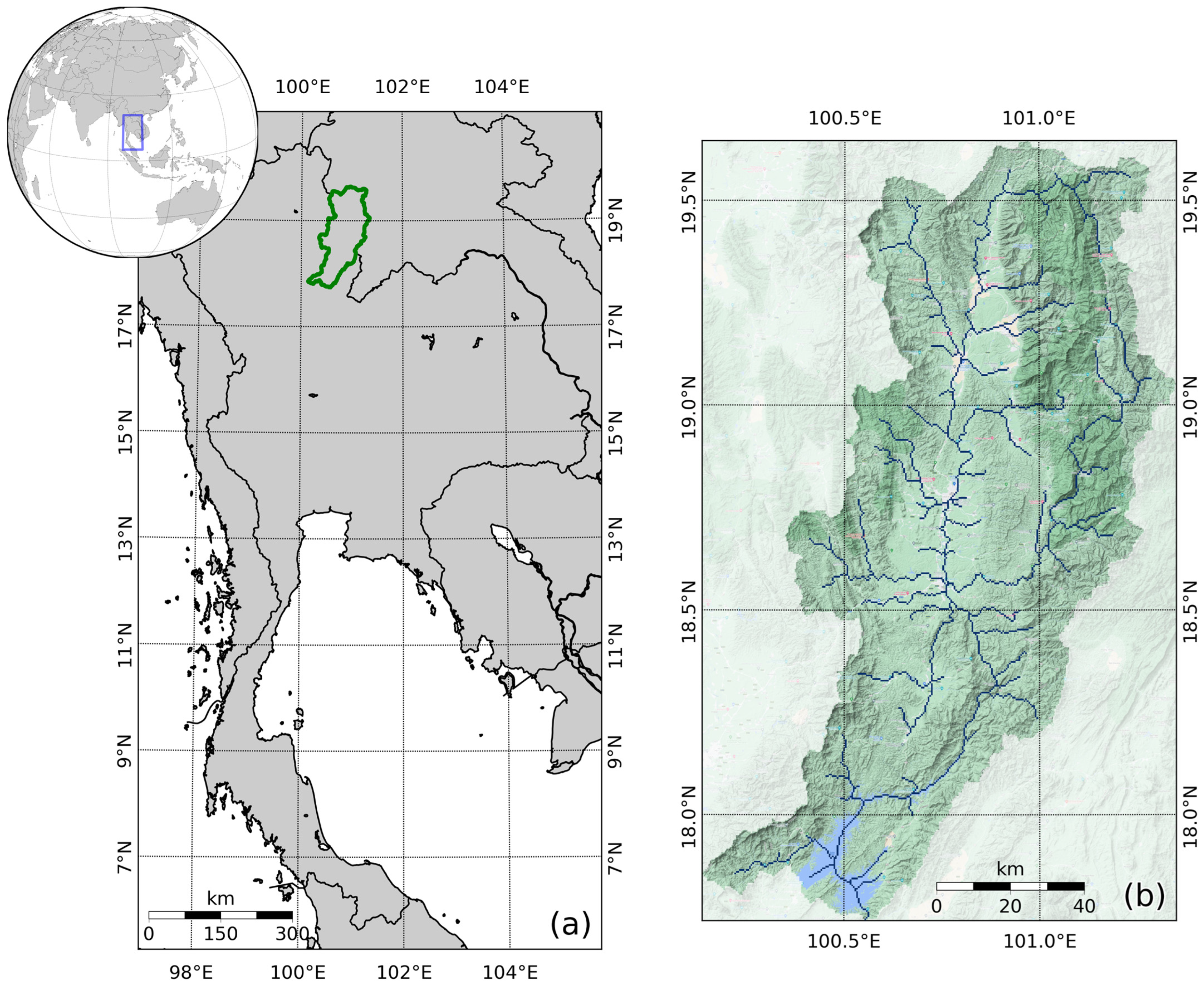
Figure 2.
Recorded precipitation from TRMM3B43V7 (NASA) in the Nan River Basin. (a) Distribution of monthly average precipitation from 2001 to 2019. (b) Average spatial precipitation in the Nan River Basin.
Figure 2.
Recorded precipitation from TRMM3B43V7 (NASA) in the Nan River Basin. (a) Distribution of monthly average precipitation from 2001 to 2019. (b) Average spatial precipitation in the Nan River Basin.
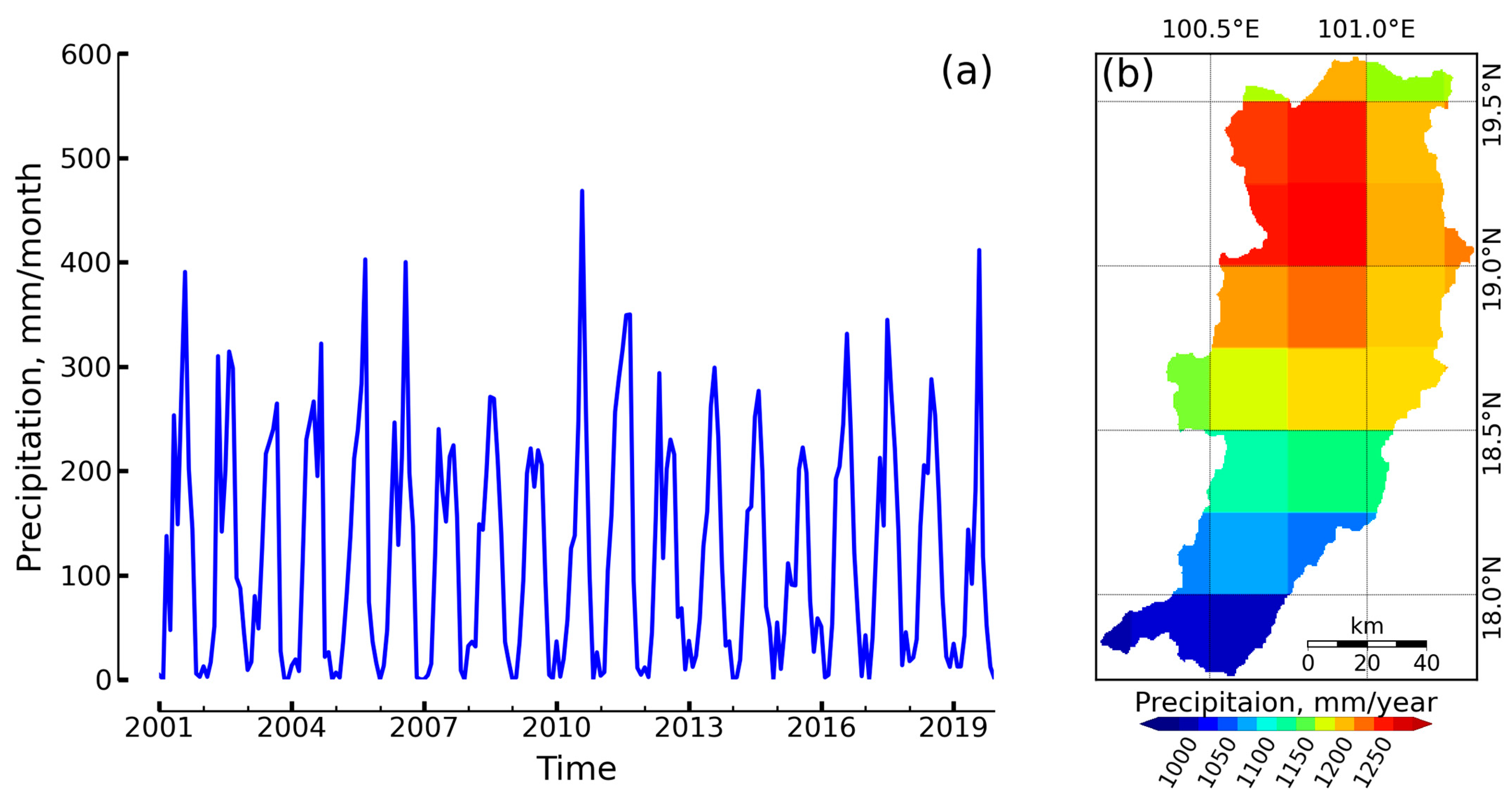
Figure 3.
Soil characteristic distribution in the Nan River Basin from the Land Development Department, Thailand, and the FAO. (a) Soil type, (b) organic carbon percentage, (c) sand percentage, (d) silt percentage, and (e) clay percentage.
Figure 3.
Soil characteristic distribution in the Nan River Basin from the Land Development Department, Thailand, and the FAO. (a) Soil type, (b) organic carbon percentage, (c) sand percentage, (d) silt percentage, and (e) clay percentage.
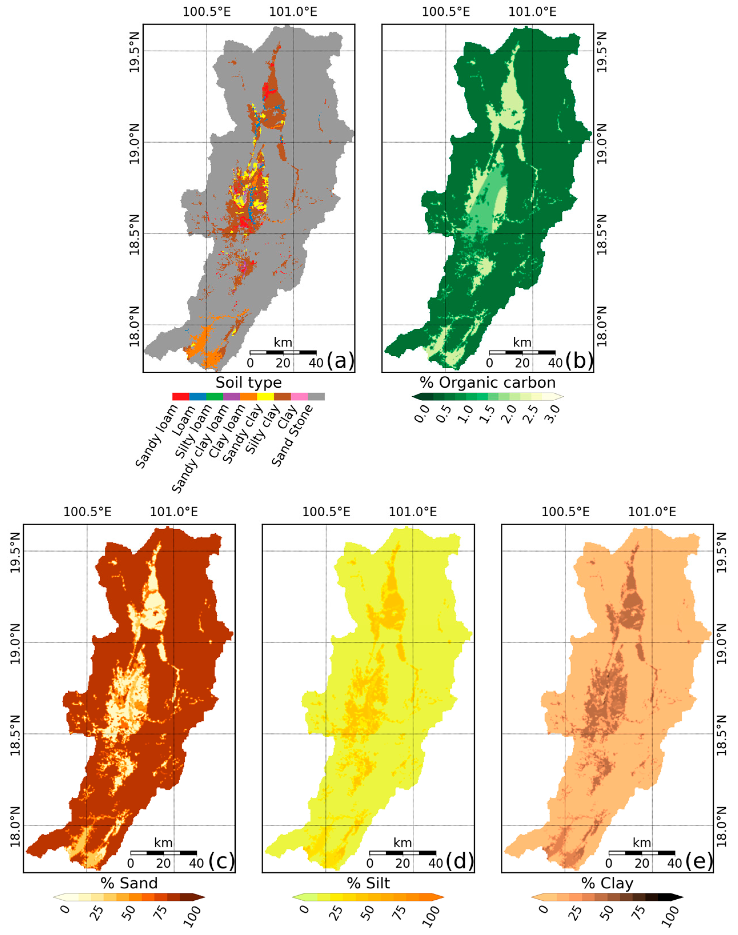
Figure 4.
Topography characteristic distribution in the Nan River Basin from SRTM. (a) Elevation, (b) slope, (c) flow direction, and (d) flow accumulation.
Figure 4.
Topography characteristic distribution in the Nan River Basin from SRTM. (a) Elevation, (b) slope, (c) flow direction, and (d) flow accumulation.
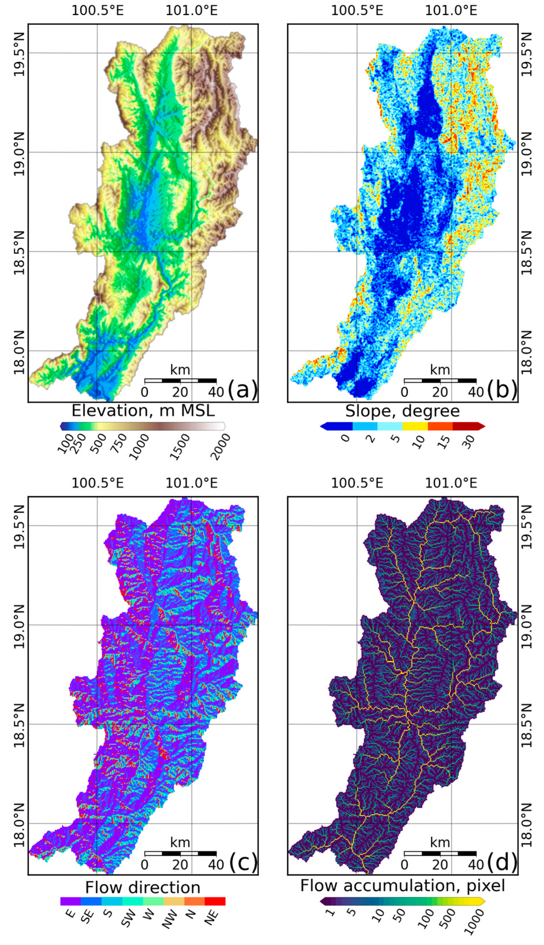
Figure 5.
Land cover distribution in the Nan River Basin from MODISMCD12Q1. (a) Land cover in 2001, (b) land cover in 2019, and (c) the difference between 2001 and 2019.
Figure 5.
Land cover distribution in the Nan River Basin from MODISMCD12Q1. (a) Land cover in 2001, (b) land cover in 2019, and (c) the difference between 2001 and 2019.

Figure 6.
Streamline of applied methodology to model the soil loss in the Nan River Basin.

Figure 7.
Spatial distribution of (a) R-factor from rainfall data, (b) K-factor from soil characteristic data, and (c) LS-factor from topography characteristic data of the Nan River Basin.
Figure 7.
Spatial distribution of (a) R-factor from rainfall data, (b) K-factor from soil characteristic data, and (c) LS-factor from topography characteristic data of the Nan River Basin.
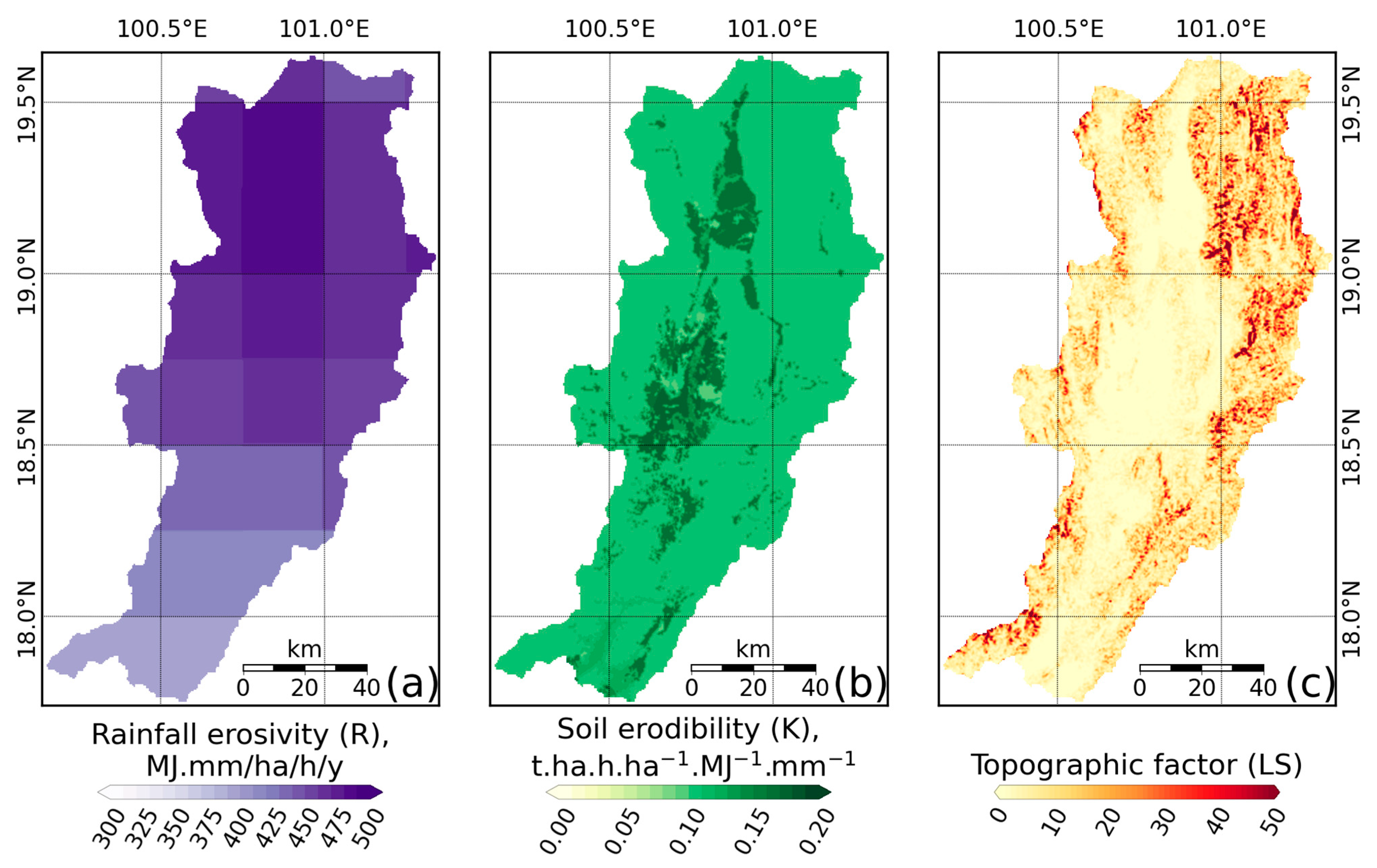
Figure 8.
Spatial distribution of (a,b) crop management (C-factor) in 2001 and 2019, respectively. (c,d) Conservation practice (P-factor) in 2001 and 2019, respectively.
Figure 8.
Spatial distribution of (a,b) crop management (C-factor) in 2001 and 2019, respectively. (c,d) Conservation practice (P-factor) in 2001 and 2019, respectively.

Figure 9.
Soil loss presented in the spatial distribution of the Nan River Basin: (a) 2001 and (b) 2019.
Figure 9.
Soil loss presented in the spatial distribution of the Nan River Basin: (a) 2001 and (b) 2019.

Figure 10.
Distribution of soil loss for each severity class in the Nan River Basin: (a) percentage area and (b) average soil loss.
Figure 10.
Distribution of soil loss for each severity class in the Nan River Basin: (a) percentage area and (b) average soil loss.
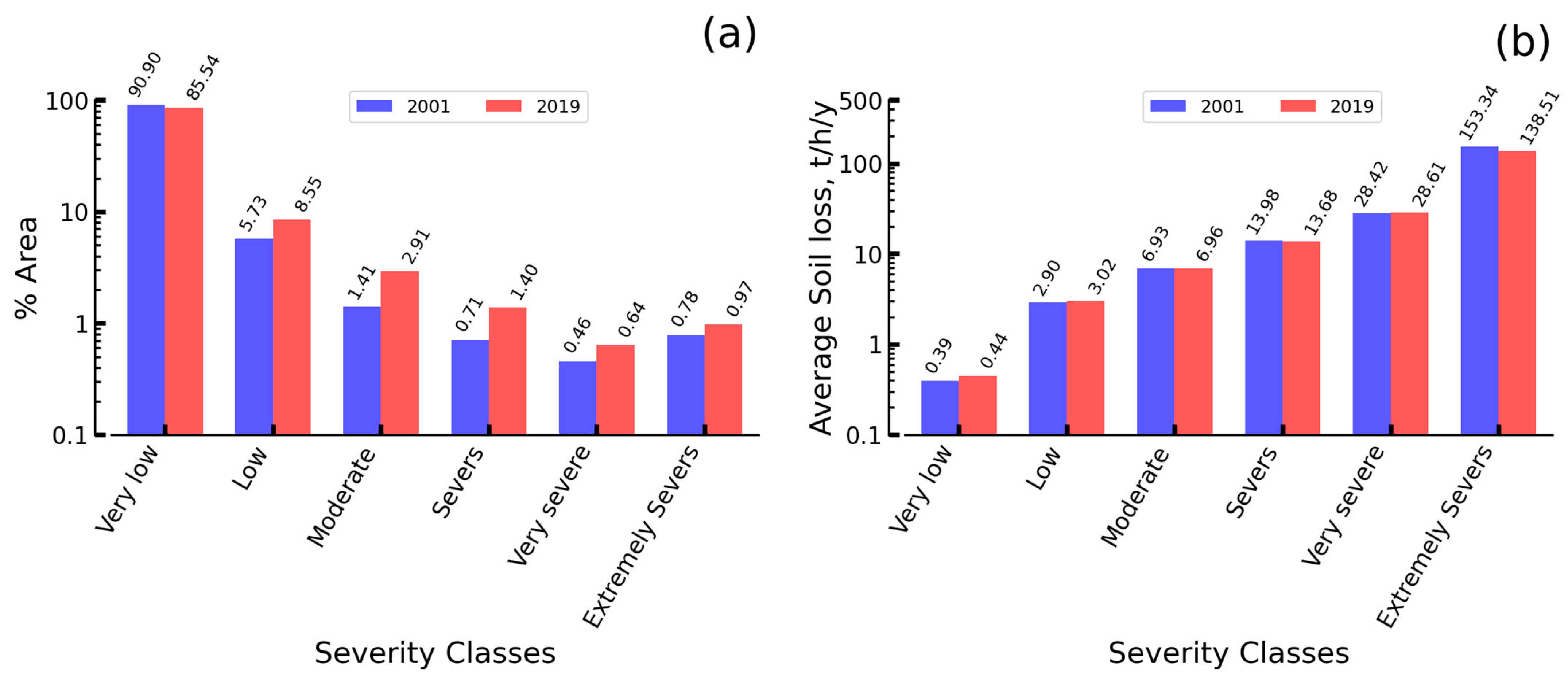
Figure 11.
Soil loss rate estimation in different elevation areas: (a) area percentage in each elevation range and (b) average soil loss rate in each elevation range.
Figure 11.
Soil loss rate estimation in different elevation areas: (a) area percentage in each elevation range and (b) average soil loss rate in each elevation range.
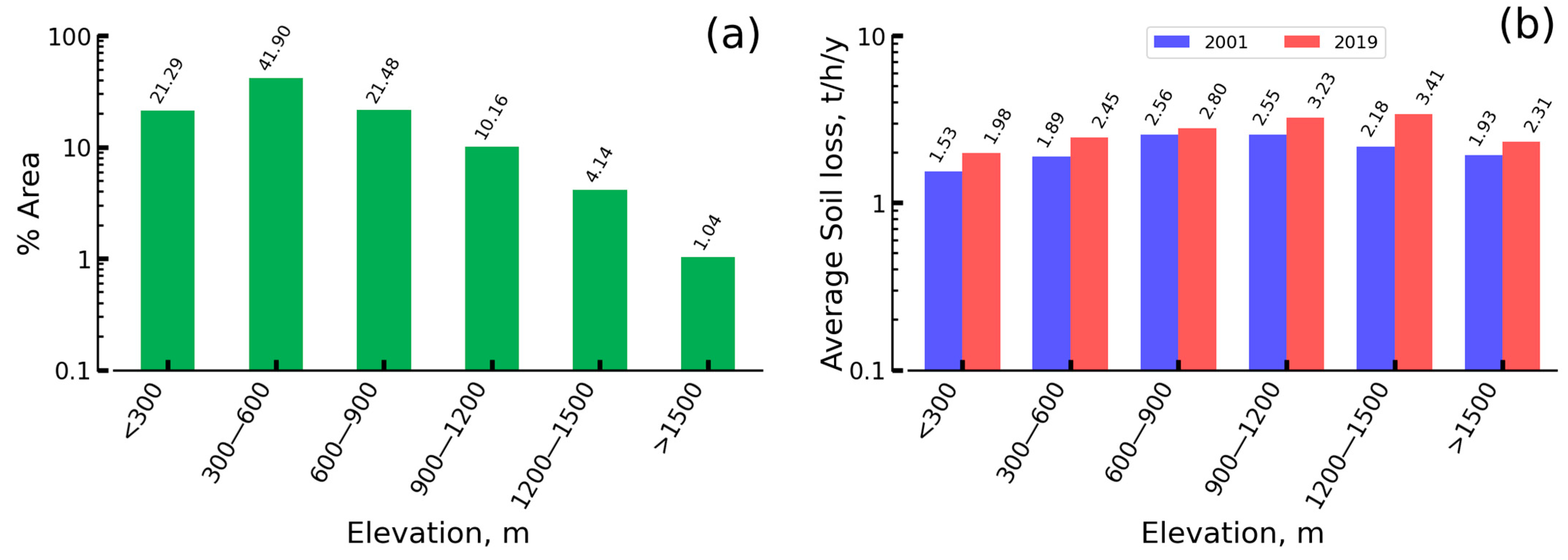
Figure 12.
Soil loss rate estimation in different slope classes: (a) area percentage in each slope class and (b) average soil loss rate in each slope class.
Figure 12.
Soil loss rate estimation in different slope classes: (a) area percentage in each slope class and (b) average soil loss rate in each slope class.

Figure 13.
Land cover change related to total soil loss in each land cover type: (a) percentage of land cover change between 2001 and 2019, (b) average soil loss for 2001 and 2019, and (c) a percentage of soil loss change between 2001 and 2019.
Figure 13.
Land cover change related to total soil loss in each land cover type: (a) percentage of land cover change between 2001 and 2019, (b) average soil loss for 2001 and 2019, and (c) a percentage of soil loss change between 2001 and 2019.


Table 1.
C- and P-factors adopted for this study are related to the land cover type.
| Land Cover Type | C-Factor | P-Factor |
|---|---|---|
| Water | 0.01 | 1.0 |
| Evergreen Forest | 0.001 | 1.0 |
| Deciduous Forest | 0.01 | 1.0 |
| Shrubland | 0.014 | 1.0 |
| Agriculture | 0.5 | 0.5 |
| Paddy | 0.1 | 0.5 |
| Urban | 0.1 | 1.0 |
| Barren | 0.35 | 1.0 |
Disclaimer/Publisher’s Note: The statements, opinions and data contained in all publications are solely those of the individual author(s) and contributor(s) and not of MDPI and/or the editor(s). MDPI and/or the editor(s) disclaim responsibility for any injury to people or property resulting from any ideas, methods, instructions or products referred to in the content. |
© 2024 by the author. Licensee MDPI, Basel, Switzerland. This article is an open access article distributed under the terms and conditions of the Creative Commons Attribution (CC BY) license (https://creativecommons.org/licenses/by/4.0/).
Share and Cite
MDPI and ACS Style
Pakoksung, K. Assessment of Soil Loss from Land Cover Changes in the Nan River Basin, Thailand. GeoHazards 2024, 5, 1-21. https://doi.org/10.3390/geohazards5010001
AMA Style
Pakoksung K. Assessment of Soil Loss from Land Cover Changes in the Nan River Basin, Thailand. GeoHazards. 2024; 5(1):1-21. https://doi.org/10.3390/geohazards5010001
Chicago/Turabian StylePakoksung, Kwanchai. 2024. "Assessment of Soil Loss from Land Cover Changes in the Nan River Basin, Thailand" GeoHazards 5, no. 1: 1-21. https://doi.org/10.3390/geohazards5010001