
Three-Dimensional Amplitude versus Offset Analysis for Gas Hydrate Identification at Woolsey Mound: Gulf of Mexico


Boone Pickens School of Geology, Oklahoma State University, 105 Noble Research Center, Stillwater, OK 74078, USA
*
Author to whom correspondence should be addressed.
GeoHazards 2024, 5(1), 271-285; https://doi.org/10.3390/geohazards5010014
Submission received: 6 February 2024
/
Revised: 26 February 2024
/
Accepted: 6 March 2024
/
Published: 8 March 2024
Abstract
:The Gulf of Mexico Hydrates Research Consortium selected the Mississippi Canyon Lease Block 118 (MC118) as a multi-sensor, multi-discipline seafloor observatory for gas hydrate research with geochemical, geophysical, and biological methods. Woolsey Mound is a one-kilometer diameter hydrate complex where gas hydrates outcrop at the sea floor. The hydrate mound is connected to an underlying salt diapir through a network of shallow crestal faults. This research aims to identify the base of the hydrate stability zone without regionally extensive bottom simulating reflectors (BSRs). This study analyzes two collocated 3D seismic datasets collected four years apart. To identify the base of the hydrate stability zone in the absence of BSRs, shallow discontinuous bright spots were targeted. These bright spots may mark the base of the hydrate stability field in the study area. These bright spots are hypothesized to produce an amplitude versus offset (AVO) response due to the trapping of free gas beneath the gas hydrate. AVO analyses were conducted on pre-stacked 3D volume and decreasing amplitude values with an increasing offset, i.e., Class 4 AVO anomalies were observed. A comparison of a time-lapse analysis and the AVO analysis was conducted to investigate the changes in the strength of the AVO curve over time. The changes in the strength are correlated with the decrease in hydrate concentrations over time.
1. Introduction
Gas hydrates consist of gas molecules, primarily methane, contained within a lattice-like structure formed by water molecules [1]. These deposits are globally distributed in shallow regions of the outer continental borders or beneath ice sheets, i.e., permafrost. These places exhibit low temperatures, relatively high pressures, and methane concentrations that exceed the solubility threshold [2,3,4]. Gas hydrates are widely acknowledged as a promising unconventional energy source for future generations, and for their potential role as geohazards [5,6]. One of the primary geohazards associated with gas hydrates is driving submarine landslides [7]. The destabilization of gas hydrates can cause a considerable increase in pore pressure by expanding in volume. This expansion leads to a drop in effective stress inside the sediment, ultimately resulting in slope failure [8,9]. Another gas hydrate-related geohazard could occur during production through hydrate-bearing zones, as hydrates could cause wellbore instability during drilling and casing collapse during production [10]. In permafrost regions, which occupy 25% of the northern hemisphere, hydrate dissociation could induce ground settlement and severe damage to infrastructures [10,11]. Moreover, the release of methane gas from destabilized hydrates can exacerbate climate change, as methane is a potent greenhouse gas [12]. Identifying gas hydrates and understanding their distribution and stability is crucial to mitigating these geohazards. Geophysical surveys, including techniques such as 2D/3D streamer seismic, cross-well seismic, multi-component ocean bottom nodes or cable surveys, vertical seismic profiling, well logging, and controlled source electromagnetic techniques, have played a crucial role in identifying and describing gas hydrate reservoirs [3,13]. These methods allow scientists to assess the spatial extent, concentration, and stability of hydrate reservoirs, providing critical information for hazard assessment and risk management.
On a seismic section, an anomalous reflector known as the bottom simulating reflector, also abbreviated as BSR, has been used to infer the presence of gas hydrates [14,15,16]. The bottom simulating reflector (BSR) is a physical contact between sediments that are rich in gas hydrates and strata that are saturated with free gas below. The BSR is frequently connected with the base of the gas hydrate stability zone (BGHSZ), and it can be characterized by imitating the shape of the seabed topography, having opposite polarity with respect to the seafloor reflection event, and having crosscutting dipping sedimentary strata. The sediments located above the BSR display high sonic velocity and amplitude blanking, whereas the sediments located beneath the BSR display high reflection strength and frequency shadow [17,18].
BSRs were first attributed to gas hydrate, occurring broadly and conspicuously along the Blake Ridge, offshore eastern North America [19,20]. Shipley et al. (1979) [21] extended this interpretation to similar features noted on continental shelves worldwide. Subsequently, BSRs of appropriate polarity and sub-seafloor depth have been considered to be reliable indicators of the position of the BGHSZ and of the occurrence of gas hydrate [14]. The majority of BSRs correspond with the BGHSZ, but there are some instances in which this is not the case. There are circumstances that can arise in which the top of free gas occurs below the BGHSZ, and the base of the gas hydrate occurs well within the gas hydrate stability zone (GHSZ) [22]. The development of BSRs requires a temperature pressure condition that does not change drastically laterally [21]. In the Gulf of Mexico, these changes occur due to complicated salt tectonics and resulting near-surface faulting [23]. As a result, the development of extensive BSRs is inhibited, thus jeopardizing the identification of the BGHSZ.
Woolsey Mound, a 1 km diameter hydrate mound, sits atop a Louann salt body, which is connected hydraulically to the mound via a series of faults and fault-related fractures [24]. The thermal conditions and the salinity of the surrounding area are primarily controlled by the salt tectonics. In Woolsey Mound, salt inhibits the development of an extensive BSR. The only seismic indicators of gas hydrate stability zones are high amplitude bright spots, which are associated with free gas accumulation in seismic data [24,25]. The absence of a BSR and lack of well-log data pose extreme challenges in the identification of the BGHSZ in the study area.
The tool employed in this study to identify the BGHSZ in the absence of a BSR is amplitude variation with offset (AVO). The difference in lithology and/or fluid content can cause variation in seismic reflection amplitude with changing source–receiver offset [26]. In recent years, this phenomenon, also known as amplitude variation with offset, has attracted much attention. Valuable clues to the fluid content can be revealed using this technique, as well as the porosity, density, and velocity of a formation. There are four different categories of AVO responses. These are as follows: Class I occurs when the strong positive zero offset reflection coefficient (Rc) decreases with offset; Class II occurs when either the small positive zero offset Rc decreases with offset or small negative zero offset Rc increases with offset; Class III occurs when the large negative zero offset Rc increases with offset; and Class IV occurs when the negative zero offset Rc decreases in magnitude with offset. This research aims to address the following objectives: using the AVO method, we aim to identify the base of the hydrate stability field by focusing on the shallow, high amplitude negative polarity BSRs at Woolsey Mound. This objective will be achieved by analyzing two 3D pre-stack datasets collected in 2010 and 2014. The second objective of this research is to characterize the dynamic nature of the hydrate system by analyzing the strength of the AVO curve collected over the interval of 4 years (2010 and 2014). The results of this study provide valuable information for identifying gas hydrates that lack BSRs and understanding their stability in the northern Gulf of Mexico.
2. Study Area
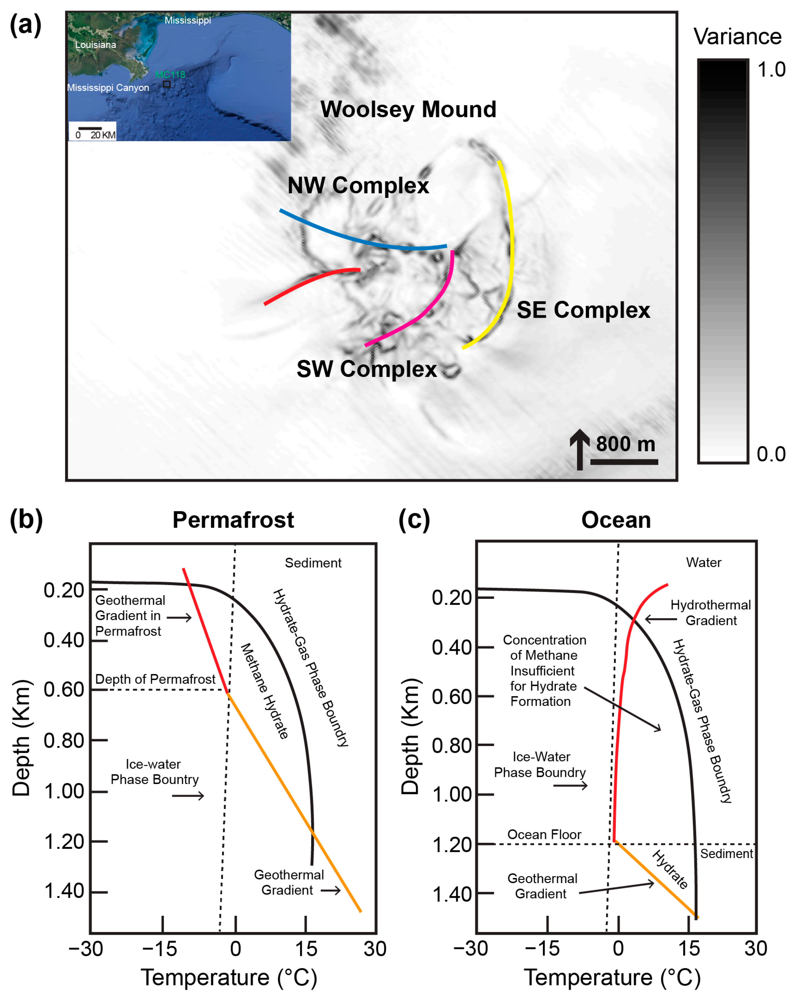
Woolsey Mound, a hydrate mound, is located in the southern portion of Mississippi Canyon Block 118 (MC118). It is located approximately 150 km south of Pascagoula, Mississippi, and 100 km east of the Mississippi Canyon in ~890 m of water (Figure 1a). The image also shows a hydrate stability phase diagram. Active seafloor venting, outcropping hydrate, and a thriving chemosynthetic community populate the seafloor in the study area. Free gas venting at the seafloor was analyzed by Sassen et al. (2006) [27]. The analysis found that the area contains C1–C5 hydrocarbons as well as CO2. The hydrate is structure II and relatively deficient in methane (70.0%) with significant ethane (7.5%) and propane (15.9%). Woolsey Mound is characterized by three main crater complexes, each 5–60 m in diameter: SE, SW, and NW crater complex [24]. Woolsey Mound sits atop an allochthonous Louann salt body. The mound evolved in close connection with the crestal fault system developed above and around the salt body [28] (Figure 1a).
Each crater complex is associated with a master fault: the NW complex is associated with the blue and red fault, the SW complex is associated with the magenta fault, and the SE complex is associated with the yellow fault [24]. These faults and fractures provide vertical migration pathways for warm hydrocarbon fluids from deeper oil reservoirs to the sea floor [28]. Macelloni et al. (2013) [29] have developed a conceptual model of the Woolsey Mound area to show the vertical migration of hydrocarbon fluid from a deep oil reservoir to the shallow subsurface via faults and fractures and accumulation in two shallow gas horizons BS-1 and BS-2. Simonetti et al. (2013) [25] developed a conceptual hydrate accumulation model based on the Jumbo Piston Core analyses and SSDR and seismic data interpretation. They concluded that hydrate formed primarily as veins and nodules in fractures in the vicinity of fault zones.
Simonetti (2013) [30] imaged the changes in the Woolsey Mound by analyzing the area close to the deeper stratigraphic horizon (BS-1). Astekin (2020) [31] studied the AVO response of the Woolsey Mound area by analyzing two seismic datasets collected in 2000 and 2003. She found that the BGHSZ produces a Class IV AVO anomaly with variation in the strength of the AVO curve over time. Astekin (2020) [31] hypothesized that these variations are due to changes in hydrate concentrations over time.
3. Materials and Methods
3.1. Data
In 2010, a 3D seismic dataset was acquired by TGS, which covers an area of 92 sq. km and has a northwest–southeast (315-degree azimuth) orientation. Another dataset used in this study was collected in 2014 with orientation and areal coverage similar to that of the 2010 dataset. These two datasets have a bin size of 30 × 25 m and a sampling rate of 4 ms. Both the 2010 and 2014 datasets were imaged 10.5 sec below the sea floor. TGS provided the depth-migrated, NMO-corrected (Normal Move Out) pre-stack 3D seismic data collected in 2010 and 2014, which will be used in the AVO study (Figure 2 and Figure 3). A 4D time-lapse processing will be conducted using the two-stacked data, where the 2010 data will be the ‘base’, and the 2014 data will be the ‘monitor’ of the study.
3.2. Methods
In this study, AVO is used to identify the base of the gas hydrate stability zone in the northern Gulf of Mexico, Woolsey Mound, which lacks a BSR. If successful, this method can be used in other areas of the Gulf of Mexico where BSRs are not regionally extensive [23]. This would aid in understanding the spatial extent of the gas hydrates and minimizing associated seafloor hazards. Two collocated pre-stack 3D seismic datasets from TGS acquired over a time interval of 4 years (2010 and 2014) were processed in this study. First, the CMP gathers 2010 and 2014 data were transformed into the angle domain (0° to 35°) from the offset domain using the velocity table created from the velocity model (Figure 4 and Figure 5). The angle transformation is carried out for a depth of 3000 m in both datasets. Then, the two-term Aki–Richards approximation [32] was used for the gradient analysis in this study. This approximation is very effective within the lower angle of incidence. The AVO analyses targeted the shallow bright spots that were hypothesized to represent the BGHSZ [24].
To test the correlation between the strength of the AVO curve and hydrate concentration, the 2014 dataset (monitor) was 4D processed to match with the 2010 dataset (baseline). The cross-equalization [33] technique was used to perform the time-lapse seismic processing. The method minimizes the differences between different surveys by removing differences in geometry, sample rate, frequency, time, phase, etc. A control window (referred to as a “static window” in this study) is chosen in a location away from the hydrate mound where pore fluid changes are less likely to occur [30]. The hydrate mound is referred to as a “dynamic window” where significant pore fluid fluctuations are expected to occur over time [30]. Time-lapse seismic monitoring using cross-equalization has been published in a range of key studies [34,35,36,37,38]. A detailed description of the processing workflow used in this study can be found in [30,33].
After minimizing all the instrumental differences, a new 3D seismic volume was created by subtracting the amplitudes of the 2014 post-4D data from the baseline 2010 data. The resulting dataset, hereafter referred to as the “difference volume”, shows the differences in seismic amplitude anomalies between the 2010 and 2014 data. As the instrumental (acquisition and processing) differences were minimized during the 4D processing sequence, these residual amplitudes are likely to reflect temporal variations in the pore–fluid content in the subsurface. The color code used here represents positive differences in orange. Since the residual volumes are created by subtracting the 4D processed volumes from the base 2010 data, orange areas identify zones of decreased amplitude over time.
4. Results and Discussions
4.1. AVO Class Identification
The AVO analyses were conducted at the shallow bright spot location in Woolsey Mound. The bright spot was analyzed in different craters at two locations in the study area. Two additional locations where AVO analyses were conducted can be found in supplementary materials (Figures S1–S7).
The first targeted area lies close to the blue and magenta faults. Figure 6 shows the map view of the area in both the 2010 and 2014 datasets. It should read–The bright spot at inline 11830 in both 2010 and 2014 is the area of interest (Figure 7).
Figure 8 and Figure 9 show the results of the AVO analyses and their associated gradient curves. The AVO curve in both figures displays a decreasing amplitude with an increasing offset, which is defined as a Class 4 AVO response [31,39]. The gradient vs. intercept crossplots show the location of the picked event in the second quadrant. This is interpreted as free gas below a high velocity layer, interpreted as gas hydrate at Woolsey Mound.
The second area of interest is located in the SE complex close to the yellow fault (Figure 6). Figure 10 displays inline 11834, which shows a distinct bright spot at a depth of 1047 m. The results of the AVO gradient analyses and corresponding crossplots are depicted in Figure 11 and Figure 12. In both figures, the gradient curve demonstrated a decreasing amplitude with increasing offset, indicating a Class 4 anomaly. The gradient versus intercept crossplots also revealed that the event of interest is located in the second quadrant.
4.2. Relationship between Hydrate Concentration and AVO Curve
The second part of the study focused on the shape/strength of the AVO curve. Astekin (2020) [31] first proposed the correlation between the strength of the AVO curve and the change in hydrate concentration, which would provide valuable information on the stability of the hydrate-bearing system to minimize associated seafloor hazards. She hypothesized that a more robust AVO response over time indicates hydrate formation, whereas a weaker response suggests dissociation over time. To test this hypothesis, a time slice from the difference volume was generated where a decrease in amplitude suggests dissociation and an increase suggests hydrate formation (Figure 13). In the study area, there are very few locations where the residual amplitude changes over time and is associated with a distinct bright spot. The AVO responses of this area are analyzed in this section to test the correlation between the strength of the AVO curve and the hydrate concentration.
The first area of interest (see ‘A’ in Figure 13) is located in the NW complex close to the blue fault. A time slice extracted above the bright spot shows a decrease in residual amplitude, implying dissociation over time. The results of the AVO analyses conducted at this bright spot from both 2010 and 2014 are displayed in Figure 14 and Figure 15, respectively. In both cases, there is a decrease in amplitude with increasing offset, which gives a Class 4 anomaly. However, the AVO curve of the 2014 dataset is significantly weaker compared to the 2010 AVO curve. The decrease in the strength of the 2014 AVO curve could be correlated with the dissociation of hydrate [31].
The second region of interest (see ‘B’ in Figure 13) is found in the NW complex adjacent to the red fault, where a drop in the residual amplitudes has been seen. The AVO analyses that were carried out at this bright spot in both 2010 and 2014 are presented in Figure 16 and Figure 17, respectively. A Class 4 anomaly is indicated when there is a decrease in amplitude with increasing offset, which occurs in both scenarios. When contrasted with the AVO curve of the 2010 data, the AVO curve of the 2014 dataset is noticeably less steep. The dissociation of hydrate may be associated with the weakening of the 2014 AVO curve.
A decrease in the residual amplitude has been observed in the third location of interest (see ‘C’ in Figure 13), which is found in the SW complex next to the magenta fault. The AVO analyses conducted at this bright spot in both 2010 and 2014 are reported in Figure 18 and Figure 19, respectively. An indicator of a Class 4 anomaly is the presence of a decrease in amplitude in conjunction with an increase in offset, which is the case in both instances. Compared to the AVO curve derived from the data collected in 2010, the AVO curve derived from the data collected in 2014 is again substantially less steep, which is hypothesized to correlate with a decrease in hydrate concentration in the area over time [29].
5. Conclusions
Understanding how gas hydrates form, their distribution, and dissociation is of paramount importance to discern their role in seafloor hazards and climate change. The lack of a discernible BSR at the BGHSZ poses a challenge in identifying the spatial extent of the gas hydrate in the northern Gulf of Mexico. The primary reason for the lack of a clearly identifiable BSR at Woolsey Mound is believed to be the intricate dynamics of salt formations, which result in fluctuations in temperature and pressure within the subsurface [24,40]. This, in turn, affects the location of the BGHSZ. The distinctive geological circumstance poses a difficulty in determining the lower boundary of the gas hydrate zone. In order to tackle this matter, the AVO analysis was employed as a seismic technique to characterize this critical boundary effectively.
This study involved the thorough analysis of two distinct sets of pre-stacked seismic recordings that were collected over a period of four years. The study’s main aim was to analyze and describe the interface separating the solid hydrates from the underlying free gas in Woolsey Mound. The interface in question is commonly characterized by a bright patch of shallow depth and negative amplitude, which has been discerned by the application of AVO analysis. The presence of this conspicuous anomaly in the seismic data serves as a clear indication of the lower boundary of the hydrate stability zone.
The analysis of AVO in the study demonstrated a consistent pattern observed in all the zones of interest characterized by bright spots. The regions mentioned above gave rise to a phenomenon referred to as a Class 4 anomaly, which is distinguished by a decline in amplitude as the offset increases. In geology, a Class 4 anomaly is characterized by the presence of a low-velocity layer, which signifies the existence of free gas beneath a high-velocity layer. In the given scenario, the high-velocity layer corresponds to gas hydrates, hence providing additional support for the application of AVO analysis in the detection of the BGHSZ [28,31,39].
A critical facet of this study involves investigating the correlation between the magnitude of the AVO curve and the change in concentration of hydrates. A time-lapse study was conducted to examine this phenomenon by comparing the two datasets gathered in 2010 and 2014. The findings from the time-lapse study revealed a progressive decline in residual amplitude as time elapsed, indicating the occurrence of hydrate dissociation. The analysis of three distinct areas of interest revealed a notable decline in the magnitude of the AVO curve in the 2014 dataset when compared to the 2010 dataset. This phenomenon has been linked to a gradual reduction in the concentration of hydrates throughout the intervening period. The discovery mentioned above significantly contributes to understanding the ever-changing characteristics of gas hydrates within this particular geographical area.
It is essential to acknowledge that the lack of shallow well-log data within the study area imposed constraints on the extent of the investigation. The inclusion of other data, such as P-wave velocity, S-wave velocity, density, and lithological information, will significantly augment the comprehension of the hydrate-bearing system and facilitate a more thorough examination of the AVO outcomes. This study’s findings suggest an opportunity for future research to expand upon the current knowledge by including a more comprehensive array of geological and geophysical data. This would contribute to a broader understanding of the dynamics of gas hydrates in this region and their role in driving landslides and climate change.
Supplementary Materials
The following supporting information can be downloaded at: https://www.mdpi.com/article/10.3390/geohazards5010014/s1, Figure S1: Map view of two additional areas (CC′ and DD′) targeted for the base of the hydrate stability zone identification using AVO analysis. The colored lines represent the master faults; Figure S2: The targeted bright spot. (a) bright spot at Inline 20389 from 2010 data and (b) bright spot at inline 20389 from 2014 data. These shallow negative polarity amplitude anomalies are hypothesized to represent the boundary separating the hydrate-bearing sediments above from free gas-bearing sediments below; Figure S3: The AVO gradient curve and associated crossplot of 2010 data at CC′. The targeted event, which occurs at 1045 m and is in the second quadrant, exhibits decreasing amplitude with increasing offset; Figure S4: The AVO gradient curve and associated crossplot of 2014 data at CC′. The targeted event, which occurs at 1046 m and is in the second quadrant, exhibits decreasing amplitude with increasing offset; Figure S5: The targeted bright spot. (a) bright spot at Inline 11820 from 2010 data and (b) bright spot at inline 11820 from 2014 data. These shallow negative polarity amplitude anomalies are hypothesized to represent the boundary separating the hydrate-bearing sediments above from free gas-bearing sediments below; Figure S6: The AVO gradient curve and associated crossplot of 2010 data at DD′. The targeted event, which occurs at 1045 m and is in the second quadrant, exhibits decreasing amplitude with increasing offset; Figure S7: The AVO gradient curve and associated crossplot of 2014 data at DD′. The targeted event, which occurs at 1050 m and is in the second quadrant, exhibits decreasing amplitude with increasing offset.
Author Contributions
Conceptualization, S.A. and C.K.; methodology, S.A.; software, S.A.; validation, S.A., C.K. and J.K.; result analysis, S.A.; writing—original draft preparation, S.A.; writing—review and editing, S.A., C.K. and J.K.; funding acquisition, C.K. and J.K. All authors have read and agreed to the published version of the manuscript.
Funding
This work was supported by the United States Department of Energy, National Energy Technology Laboratory, through Cooperative Agreement DEFE0031557, CFDA 81.089, with the Southern States Energy Board. Cost share and research support were provided by the Project Partners and an Advisory Committee.
Data Availability Statement
The data are not publicly available due to privacy issues.
Acknowledgments
The authors are grateful to TGS-Nopec for providing the seismic data. This project has been supported by Southeast Regional Carbon Storage Partnership: Offshore Gulf of Mexico.
Conflicts of Interest
The authors declare no conflicts of interest. The funders had no role in the design of the study; in the collection, analyses, or interpretation of data; in the writing of the manuscript; or in the decision to publish the results.
References
- Sloan, E.D. Gas hydrates: Review of Physical/Chemical Properties. Energy Fuels 1998, 12, 191–196. [Google Scholar] [CrossRef]
- Sloan, E.D. Fundamental principles and applications of natural gas hydrates. Nature 2003, 426, 353–359. [Google Scholar] [CrossRef] [PubMed]
- Paull, C.K.; Dillon, W.P. Natural Gas Hydrates: Occurrence, Distribution, and Detection; Geophysical Monograph Series; American Geophysical Union: Washington, DC, USA, 2001; Volume 124. [Google Scholar]
- Milkov, A.V.; Dickens, G.R.; Claypool, G.E.; Lee, Y.J.; Borowski, W.S.; Torres, M.E.; Xu, W.; Tomaru, H.; Tréhu, A.M.; Schultheiss, P. Co-existence of gas hydrate, free gas, and brine within the regional gas hydrate stability zone at Hydrate Ridge (Oregon margin): Evidence from prolonged degassing of a pressurized core. Earth Planet. Sci. Lett. 2004, 222, 829–843. [Google Scholar] [CrossRef]
- Boswell, R.; Collett, T.S. Current perspectives on gas hydrate resources. Energy Environ. Sci. 2011, 4, 1206–1215. [Google Scholar] [CrossRef]
- Collett, T.S. Gas hydrates as a future energy resource. Geotimes 2004, 49, 24–27. [Google Scholar]
- Kvenvolden, K.A. Gas hydrates-Geological perspective and global change. Rev. Geophys. 1993, 31, 173–187. [Google Scholar] [CrossRef]
- McIver, R.D. Role of naturally occurring gas hydrates in sediment transport. AAPG Bull. 1982, 66, 789–792. [Google Scholar] [CrossRef]
- Nixon, F.M.; Grozic, J.L.H. Submarine slope failure due to gas hydrate dissociation: A preliminary quantification. Can. Geotech. J. 2007, 44, 314–325. [Google Scholar] [CrossRef]
- Farahani, M.V.; Hassanpourypuzband, A.; Yang, J.; Tohidi, B. Insights into the climate-driven evolution of gas hydrate-bearing permafrost sediments: Implications for prediction of environmental impacts and security of energy in cold regions. RSC Adv. 2021, 11, 14334–14346. [Google Scholar] [CrossRef]
- Farahani, M.V.; Hassanpourypuzband, A.; Yang, J.; Tohidi, B. Development of a coupled geophysical–geothermal scheme for quantification of hydrates in gas hydrate-bearing permafrost sediments. Phys. Chem. Chem. Phys. 2021, 23, 24249–24264. [Google Scholar] [CrossRef]
- Intergovernmental Panel on Climate Change (IPCC). Climate Change 2013: The Physical Science Basis. Contribution of Working Group I to the Fifth Assessment Report of the Intergovernmental Panel on Climate Change; Cambridge University Press: Cambridge, UK, 2013. [Google Scholar]
- Riedel, M.; Willoughby, E.C.; Chopra, S. (Eds.) Geophysical Characterization of Gas Hydrates; Society of Exploration Geophysicists: Houston, TX, USA, 2010. [Google Scholar]
- Hyndman, R.D.; Spence, G.D. A seismic study of methane hydrate marine bottom simulating reflectors. J. Geophys. Res. Solid Earth 1992, 97, 6683–6698. [Google Scholar] [CrossRef]
- Singh, S.C.; Minshull, T.A.; Spence, G.D. Velocity Structure of a Gas Hydrate Reflector. Science 1993, 260, 204–207. [Google Scholar] [CrossRef]
- Sriram, G.; Dewangan, P.; Ramprasad, T.; Rama Rao, P. Anisotropic amplitude variation of the bottom-simulating reflector beneath fracture-filled gas hydrate deposit. J. Geophys. Res. 2013, 118, 2258–2274. [Google Scholar] [CrossRef]
- Sain, K.; Minshull, T.A.; Singh, S.C.; Hobbs, R.W. Evidence for a thick free gas layer beneath the bottom simulating reflector in the Makran accretionary prism. Mar. Geol. 2000, 164, 3–12. [Google Scholar] [CrossRef]
- Satyavani, N.; Sain, K.; Lall, M.; Kumar, B. Seismic attribute study for gas hydrates in the Andaman Offshore India. Mar. Geophys. Res. 2008, 29, 167–175. [Google Scholar] [CrossRef]
- Bryan, G.M. In Situ Indications of Gas Hydrate. In Natural Gases in Marine Sediments; Kaplan, I.R., Ed.; Springer: Greer, SC, USA, 1974; pp. 299–308. [Google Scholar] [CrossRef]
- Tucholke, B.E.; Bryan, G.M.; Ewing, J.I. Gas-hydrate horizons detected in seismic-profiler data from the Western North Atlantic. Am. Assoc. Pet. Geol. Bull. 1977, 61, 698–707. [Google Scholar] [CrossRef]
- Shipley, T.H. Seismic evidence for widespread possible gas hydrate horizons on continental slopes and rises. Am. Assoc. Pet. Geol. Bull. 1977, 63, 2204–2213. [Google Scholar]
- Xu, W.; Ruppel, C. Predicting the occurrence, distribution, and evolution of methane gas hydrate in porous marine sediments. J. Geophys. Res. 1999, 104, 5081–5096. [Google Scholar] [CrossRef]
- Shedd, W.; Boswell, R.; Frye, M.; Godfriaux, P.; Kramer, K. Occurrence and nature of “bottom simulating reflectors” in the northern Gulf of Mexico. Mar. Pet. Geol. 2012, 34, 31–40. [Google Scholar] [CrossRef]
- Macelloni, L.; Simonetti, A.; Knapp, J.H.; Knapp, C.C.; Lutken, C.B.; Lapham, L.L. Multiple resolution seismic imaging of a shallow hydrocarbon plumbing system, Woolsey Mound, Northern Gulf of Mexico. Mar. Pet. Geol. 2012, 38, 128–142. [Google Scholar] [CrossRef]
- Simonetti, A.; Knapp, J.H.; Sleeper, K.; Lutken, C.B.; Macelloni, L.; Knapp, C.C. Spatial distribution of gas hydrates from high-resolution seismic and core data, Woolsey Mound, Northern Gulf of Mexico. Mar. Pet. Geol. 2013, 44, 21–33. [Google Scholar] [CrossRef]
- Castagna, J.P.; Swan, H.W.; Foster, D.J. Framework for AVO gradient and intercept interpretation. Geophysics 1998, 63, 948–956. [Google Scholar] [CrossRef]
- Sassen, R.; Roberts, H.H.; Jung, W.; Lutken, C.B.; DeFreitas, D.A.; Sweet, S.T.; Guinasso, N.L., Jr. The Mississippi Canyon 118 Gas Hydrate Site: A Complex Natural System. In Proceedings of the Offshore Technology Conference, Houston, TX, USA, 1–4 May 2006. [Google Scholar] [CrossRef]
- Knapp, J.; Knapp, C.; Macelloni, L.; Simonetti, A.; Lutken, C. Subsurface structure and stratigraphy of a transient, fault-controlled thermogenic hydrate system at MC-118. In Proceedings of the AAPG Annual Convention and Exhibition, New Orleans, LA, USA, 11–14 April 2010. [Google Scholar]
- Macelloni, L.; Brunner, C.A.; Caruso, S.; Lutken, C.B.; Lapham, L.L. Spatial distribution of seafloor bio-geological and geochemical processes as proxies of fluid flux regime and evolution of a carbonate/hydrates mound, northern Gulf of Mexico. Deep. -Sea Res. Part I 2013, 74, 25–38. [Google Scholar] [CrossRef]
- Simonetti, A. Spatial and Temporal Characterization of a Cold Seep-Hydrate System (Woolsey Mound, Deep-Water Gulf of Mexico). Ph.D. Dissertation, University of South Carolina, Columbia, SC, USA, 2013. [Google Scholar]
- Astekin, G. 3-D Amplitude versus Offset Analysis for Gas Hydrate Identification in the Northern Gulf of Mexico: Woolsey Mound. Master’s Thesis, Oklahoma State University, Stillwater, OK, USA, 2020. [Google Scholar]
- Aki, K.; Richards, P.G. Quantitative Seismology: Theory and Methods; W. H. Freeman and Co.: San Francisco, CA, USA, 1980. [Google Scholar]
- Riedel, M. 4D seismic time-lapse monitoring of an active cold vent, northern Cascadia margin. Mar. Geophys. Res. 2007, 28, 355–371. [Google Scholar] [CrossRef]
- Burkhart, T.; Hoover, A.R.; Flemings, P.B. Time-lapse seismic monitoring of the South Timbalier 295 field, offshore Louisiana. In SEG Technical Program Expanded Abstracts; Society of Exploration Geophysicists: Houston, TX, USA, 1997; pp. 910–913. [Google Scholar]
- Eastwood, J.; Johnston, D.; Huang, X.; Craft, K.; Workman, R. Processing for robust time-lapse seismic analysis: Gulf of Mexico example, Lena field. In SEG Technical Program Expanded Abstracts; Society of Exploration Geophysicists: Houston, TX, USA, 1998; pp. 20–23. [Google Scholar]
- Eastwood, J.; Johnston, D.H.; Shyeh, J.; Huang, X.; Craft, K.; Vauthrin, R.; Workman, R. Time-lapse seismic processing and analysis: Gulf of mexico example, lena field. In Proceedings of the Offshore Technology Conference, Houston, TX, USA, 3–6 May 1999. [Google Scholar]
- Ross, C.P.; Altan, M.S. Time-lapse seismic monitoring: Some shortcomings in nonuniform processing. Lead. Edge 1997, 16, 931–937. [Google Scholar] [CrossRef]
- Rickett, J.; Lumley, D.E. A cross-equalization processing flow for off-the-shelf 4D seismic data. In SEG Technical Program Expanded Abstracts; Society of Exploration Geophysicists: Houston, TX, USA, 1998; pp. 16–19. [Google Scholar]
- Diaconescu, C.C.; Knapp, J.H. Buried Gas Hydrates in the Deepwater of the South Caspian Sea, Azerbaijan: Implications for Geo-Hazards. Energy Explor. Exploit. 2000, 18, 385–400. [Google Scholar] [CrossRef]
- Macelloni, L.; Lutken, C.B.; Garg, S.; Simonetti, A.; D’Emidio, M.; Wilson, R.M.; McGee, T.M. Heat-flow regimes and the hydrate stability zone of a transient, thermogenic, fault-controlled hydrate system (Woolsey Mound northern Gulf of Mexico). Mar. Pet. Geol. 2015, 59, 491–504. [Google Scholar] [CrossRef]
Figure 1.
Woolsey Mound is located in Mississippi Canyon Lease Block 118 on the northeastern Gulf of Mexico continental slope. (a) The study area is displayed on a variance plot extracted from the seafloor. The mound is subdivided into three crater complexes. Each complex is associated with a master fault (colored lines) that connects the underlying salt body to the seafloor. (b) Gas hydrate stability zone phase diagram in permafrost and (c) ocean.

Figure 2.
Pre-stack depth-migrated NMO-corrected 3D seismic data collected in 2010.
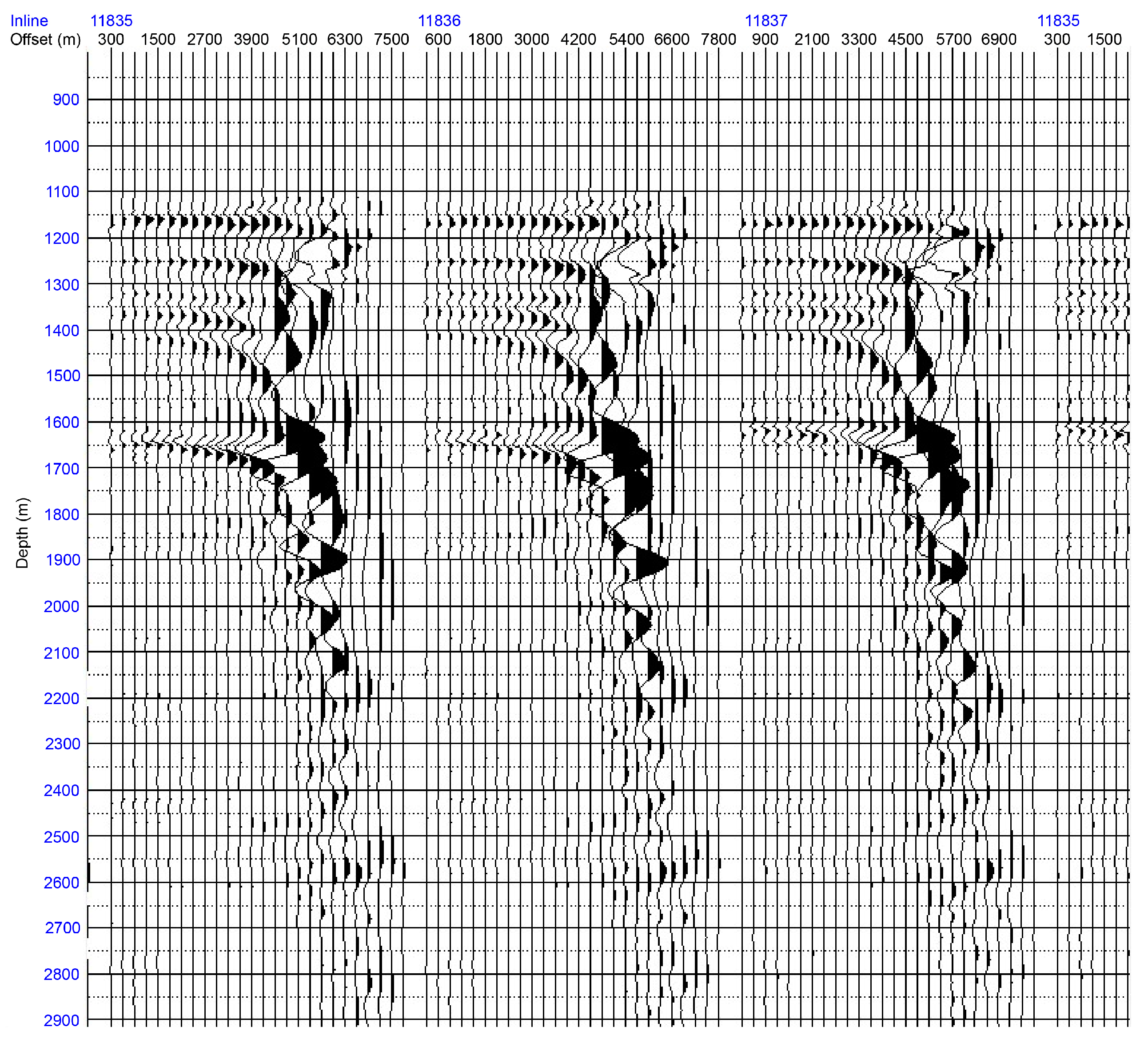
Figure 3.
Pre-stack depth-migrated NMO-corrected 3D seismic data collected in 2014.

Figure 4.
Angle-transformed 2010 dataset.
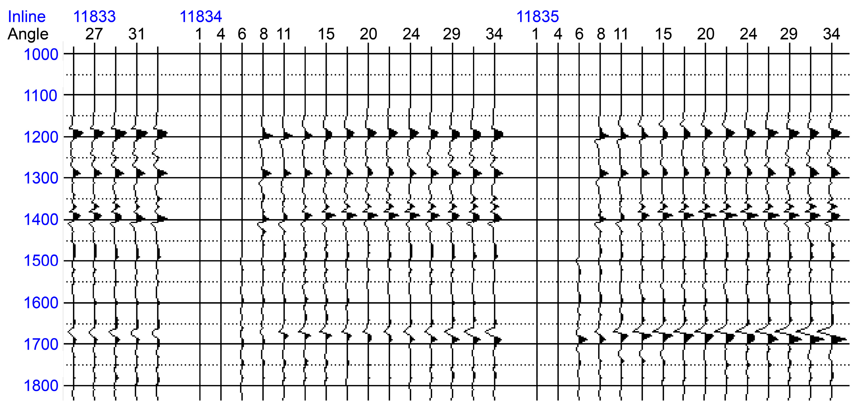
Figure 5.
Angle-transformed 2014 dataset.
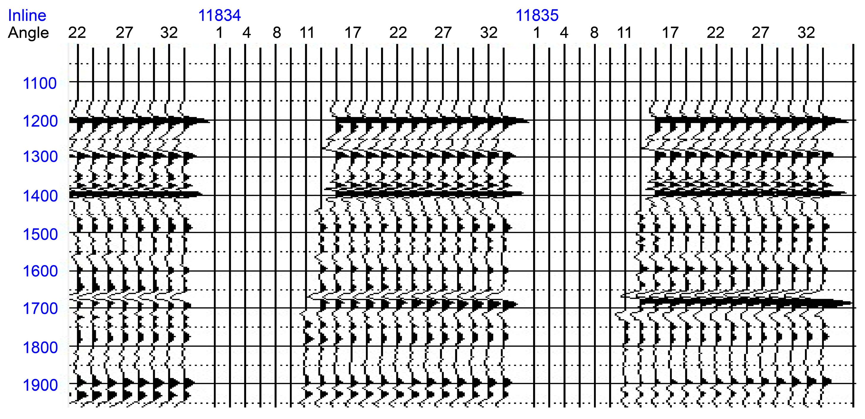
Figure 6.
Map view of the area targeted for AVO analysis. The colored lines represent the master faults.
Figure 6.
Map view of the area targeted for AVO analysis. The colored lines represent the master faults.
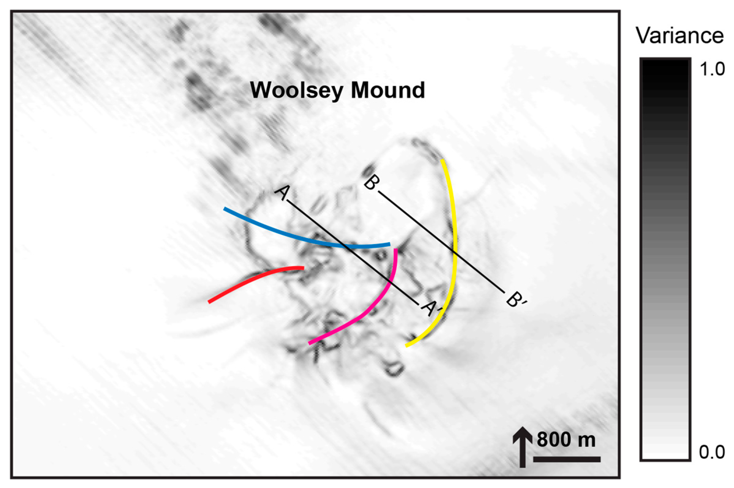
Figure 7.
The targeted bright spot. (a) bright spot at inline 11830 from 2010 data and (b) bright spot at inline 11830 from 2014 data. These shallow negative polarity amplitude anomalies are hypothesized to represent the boundary separating the hydrate-bearing sediments above from free gas-bearing sediments below.
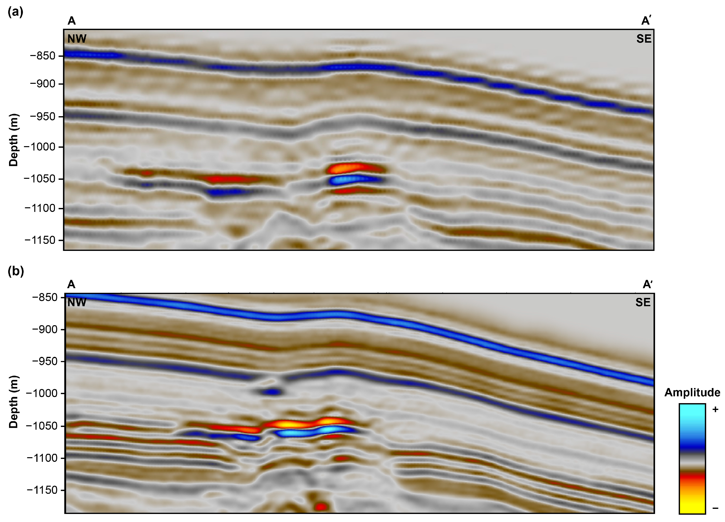
Figure 8.
The AVO gradient curve and associated crossplot of 2010 data. The targeted event, which occurs at 1045 m and is in the second quadrant, exhibits decreasing amplitude with increasing offset.
Figure 8.
The AVO gradient curve and associated crossplot of 2010 data. The targeted event, which occurs at 1045 m and is in the second quadrant, exhibits decreasing amplitude with increasing offset.
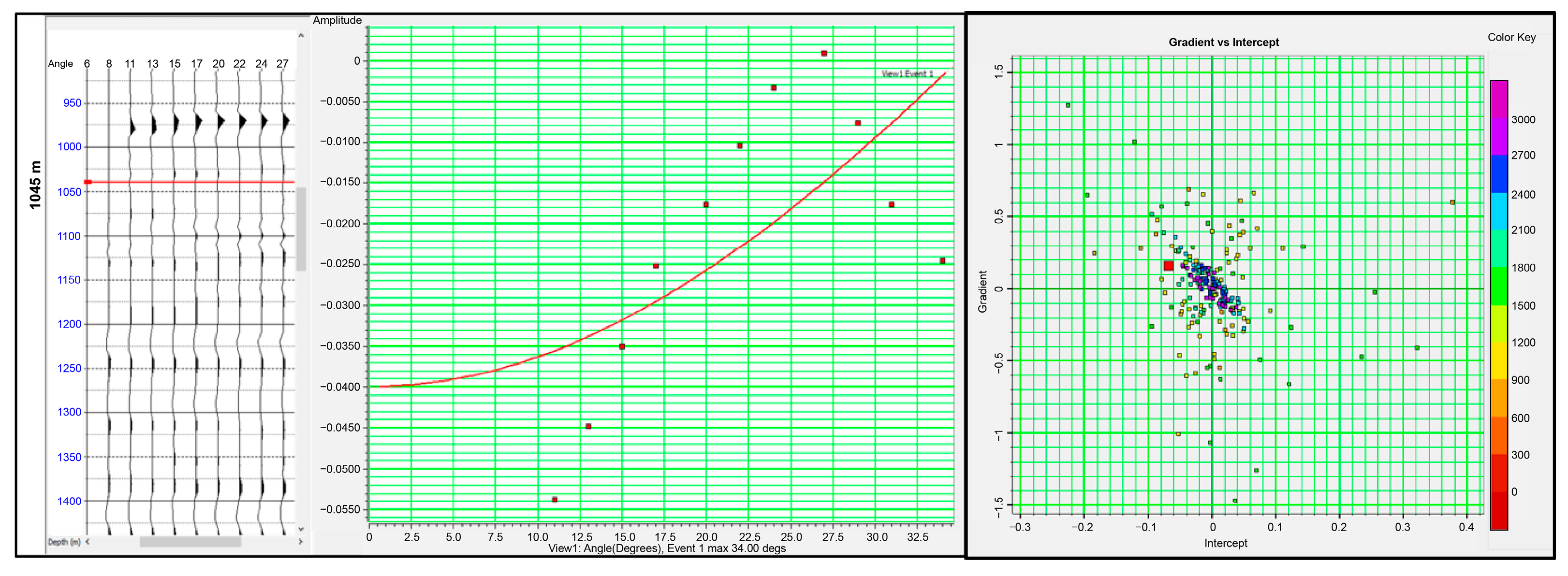
Figure 9.
The AVO gradient curve and associated crossplot of 2014 data. The targeted event, which occurs at 1048 m and is in the second quadrant, exhibits decreasing amplitude with increasing offset.
Figure 9.
The AVO gradient curve and associated crossplot of 2014 data. The targeted event, which occurs at 1048 m and is in the second quadrant, exhibits decreasing amplitude with increasing offset.
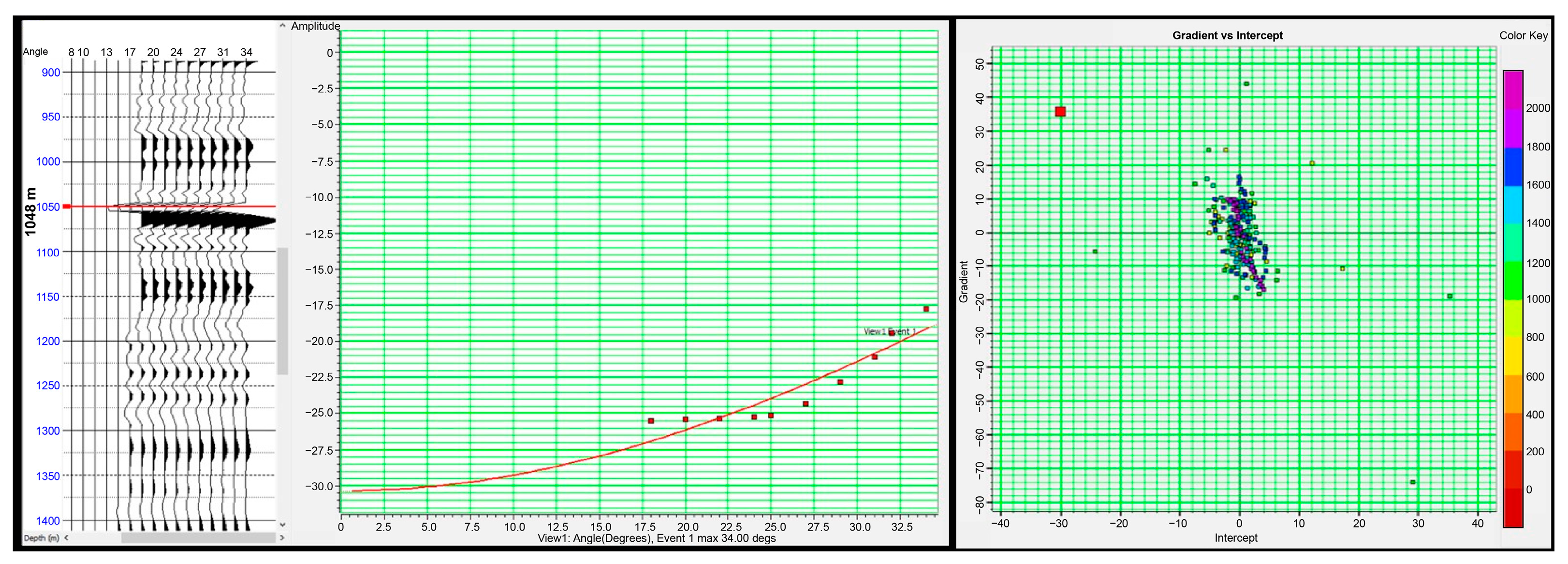
Figure 10.
The targeted bright spot. (a) bright spot at inline 11834 from 2010 data and (b) bright spot at inline 11834 from 2014 data. These shallow negative polarity amplitude anomalies are hypothesized to represent the boundary separating the hydrate-bearing sediments above from free gas-bearing sediments below.
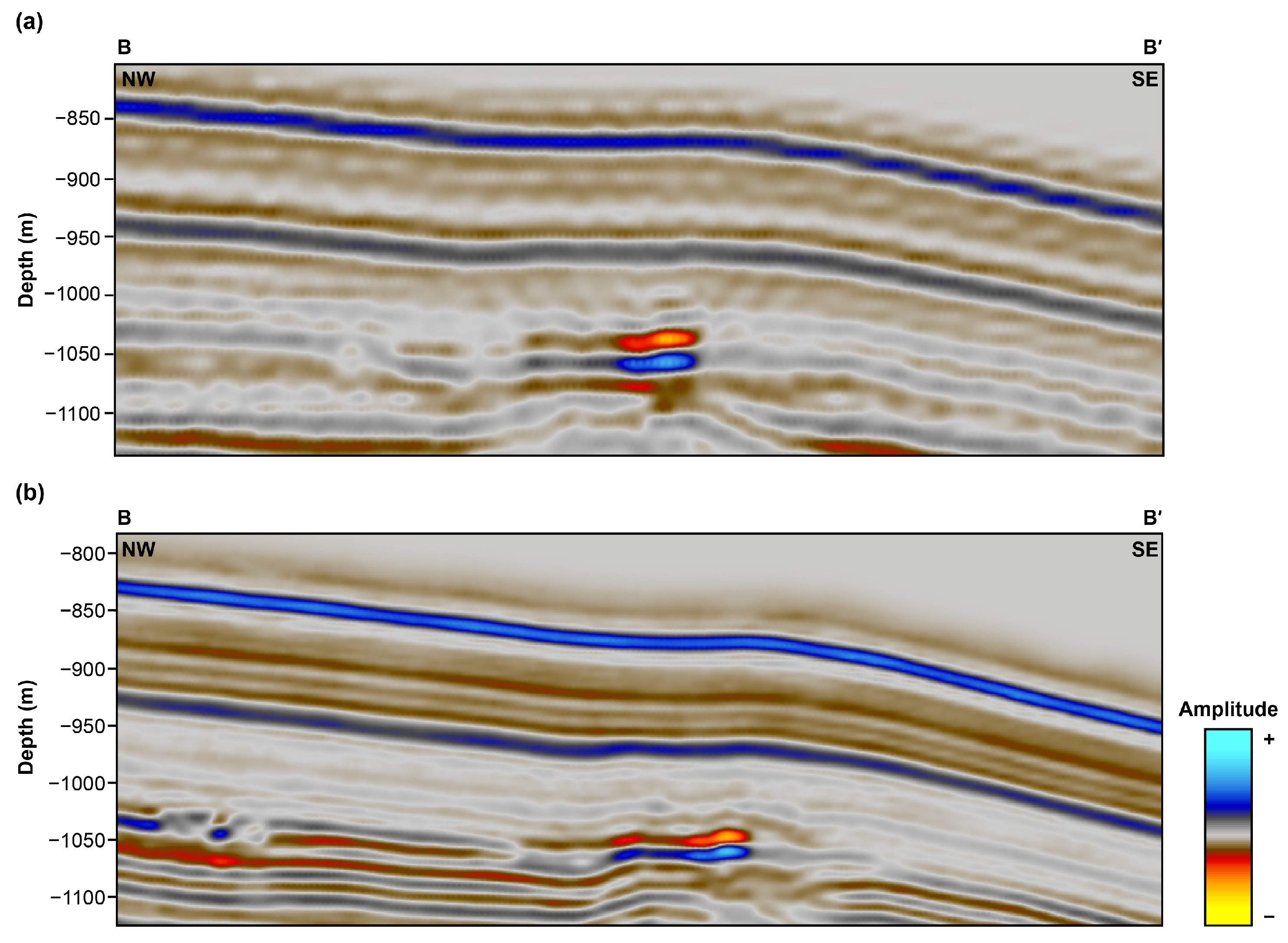
Figure 11.
The AVO gradient curve and associated crossplot of 2010 data. The targeted event, which occurs at 1045 m and is in the second quadrant, exhibits decreasing amplitude with increasing offset.
Figure 11.
The AVO gradient curve and associated crossplot of 2010 data. The targeted event, which occurs at 1045 m and is in the second quadrant, exhibits decreasing amplitude with increasing offset.
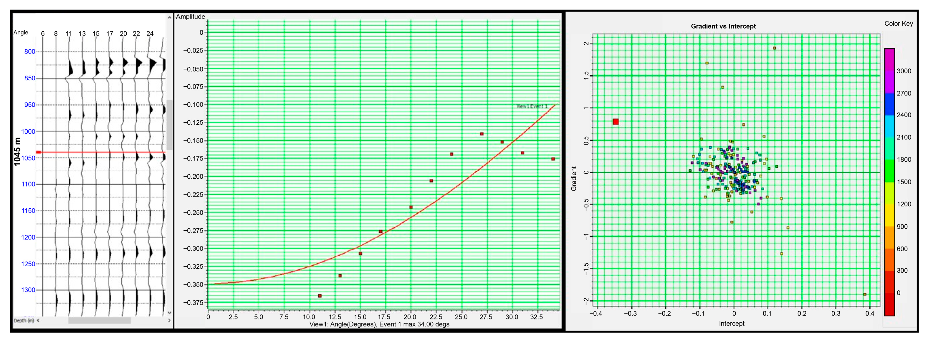
Figure 12.
The AVO gradient curve and associated crossplot of 2014 data. The targeted event, which occurs at 1050 m and is in the second quadrant, exhibits decreasing amplitude with increasing offset.
Figure 12.
The AVO gradient curve and associated crossplot of 2014 data. The targeted event, which occurs at 1050 m and is in the second quadrant, exhibits decreasing amplitude with increasing offset.
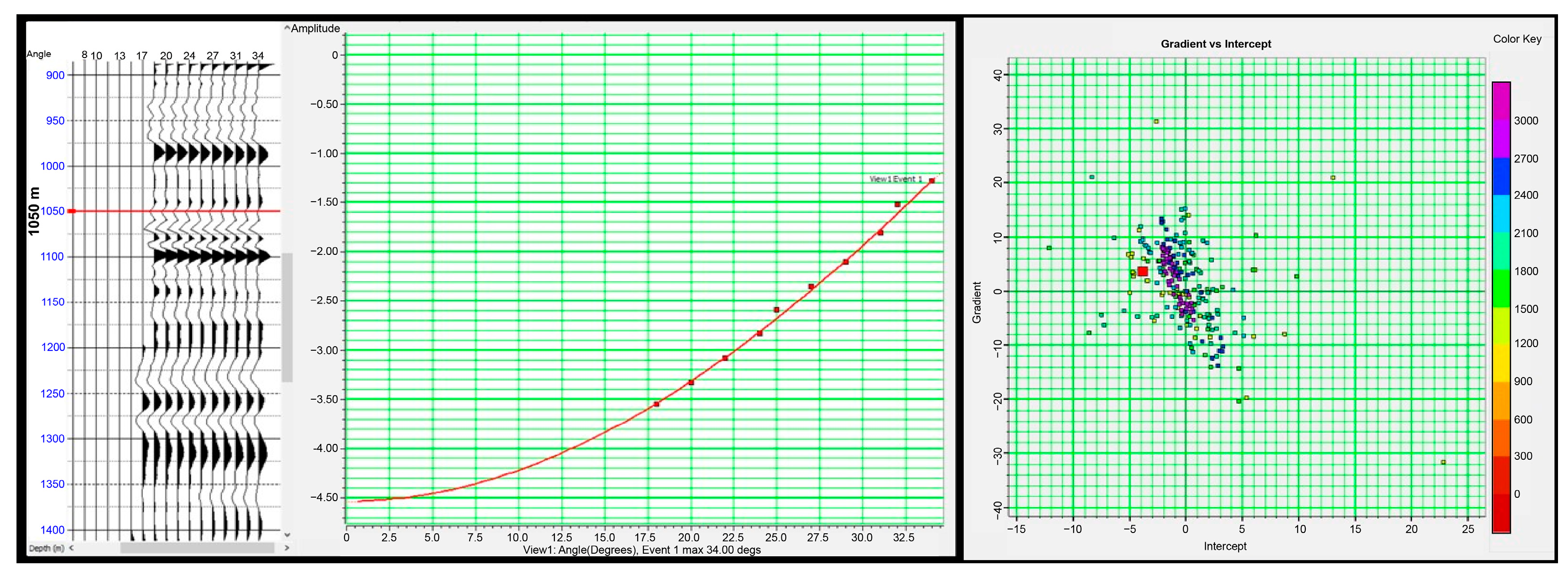
Figure 13.
A time slice extracted from the difference volume to show changes in amplitudes over 4 years. The orange areas in the mound are interpreted as zones of decreased amplitudes (hydrate dissociation), and the blue areas are interpreted as zones of increased amplitudes (hydrate formation). The colored lines represent the master faults connecting the mound to the underlying salt body. Static window—an area away from the hydrate mound where pore fluid changes are less likely. Dynamic window—an area surrounding the hydrate mound where pore fluid changes are expected over time. A, B, and C depict the areas of interest for AVO analysis.
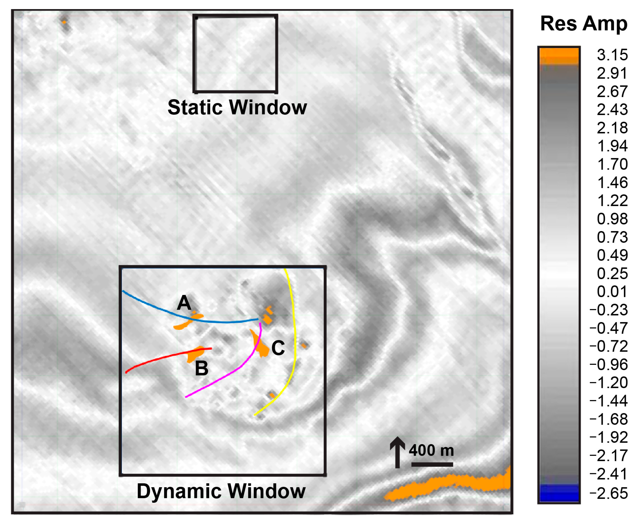
Figure 14.
The AVO gradient curve and associated crossplot of 2010 data. The targeted event, which occurs at 1045 m and is in the second quadrant, exhibits decreasing amplitude with increasing offset.
Figure 14.
The AVO gradient curve and associated crossplot of 2010 data. The targeted event, which occurs at 1045 m and is in the second quadrant, exhibits decreasing amplitude with increasing offset.
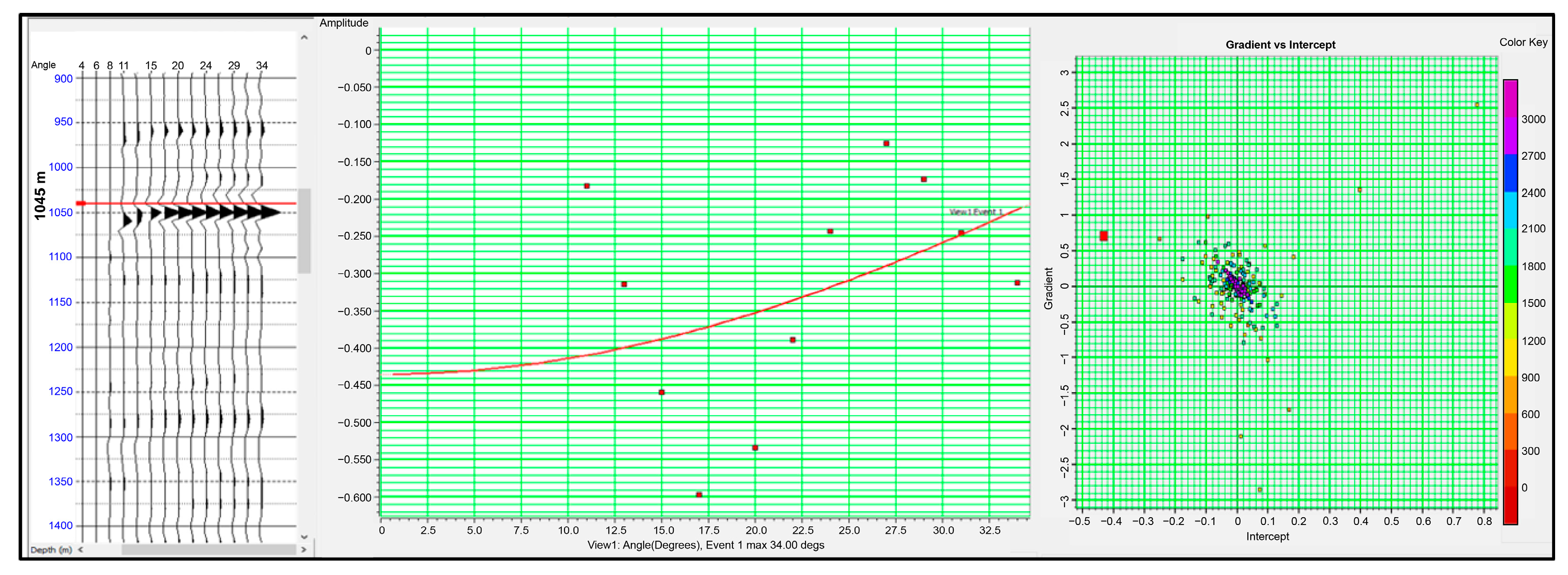
Figure 15.
The AVO gradient curve and associated crossplot of 2014 data. The targeted event, which occurs at 1050 m and is in the second quadrant, exhibits decreasing amplitude with increasing offset. Note a sharp decrease in the strength of the AVO curve compared to 2010 data.
Figure 15.
The AVO gradient curve and associated crossplot of 2014 data. The targeted event, which occurs at 1050 m and is in the second quadrant, exhibits decreasing amplitude with increasing offset. Note a sharp decrease in the strength of the AVO curve compared to 2010 data.
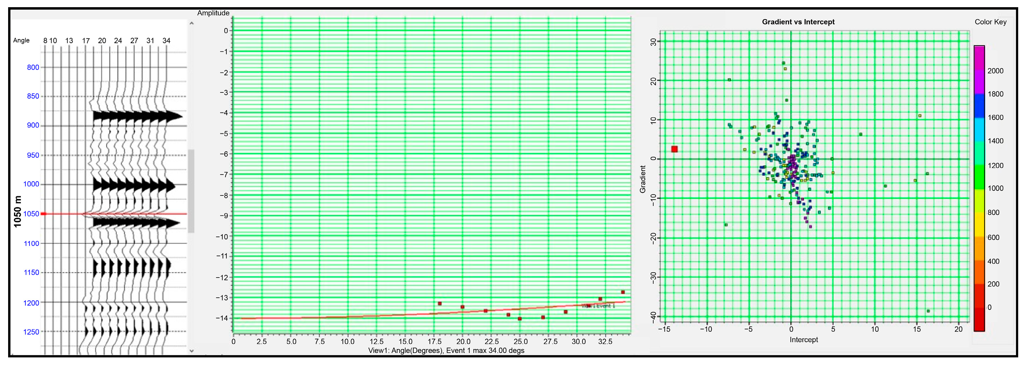
Figure 16.
The AVO gradient curve and associated crossplot of 2010 data. The targeted event, which occurs at 1040 m and is in the second quadrant, exhibits decreasing amplitude with increasing offset.
Figure 16.
The AVO gradient curve and associated crossplot of 2010 data. The targeted event, which occurs at 1040 m and is in the second quadrant, exhibits decreasing amplitude with increasing offset.

Figure 17.
The AVO gradient curve and associated crossplot of 2014 data. The targeted event, which occurs at 1047 m and is in the second quadrant, exhibits decreasing amplitude with increasing offset. Note a sharp decrease in the strength of the AVO curve compared to 2010 data.
Figure 17.
The AVO gradient curve and associated crossplot of 2014 data. The targeted event, which occurs at 1047 m and is in the second quadrant, exhibits decreasing amplitude with increasing offset. Note a sharp decrease in the strength of the AVO curve compared to 2010 data.
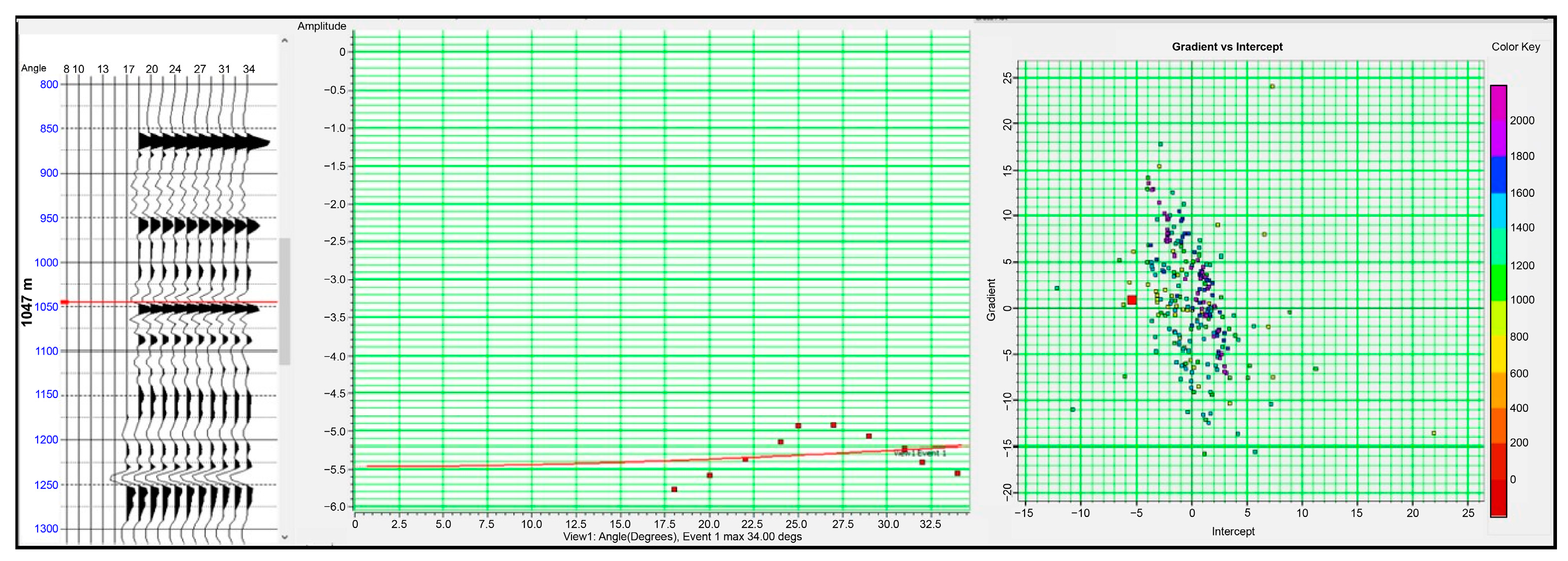
Figure 18.
The AVO gradient curve and associated crossplot of 2010 data. The targeted event, which occurs at 1047 m and is in the second quadrant, exhibits decreasing amplitude with increasing offset.
Figure 18.
The AVO gradient curve and associated crossplot of 2010 data. The targeted event, which occurs at 1047 m and is in the second quadrant, exhibits decreasing amplitude with increasing offset.
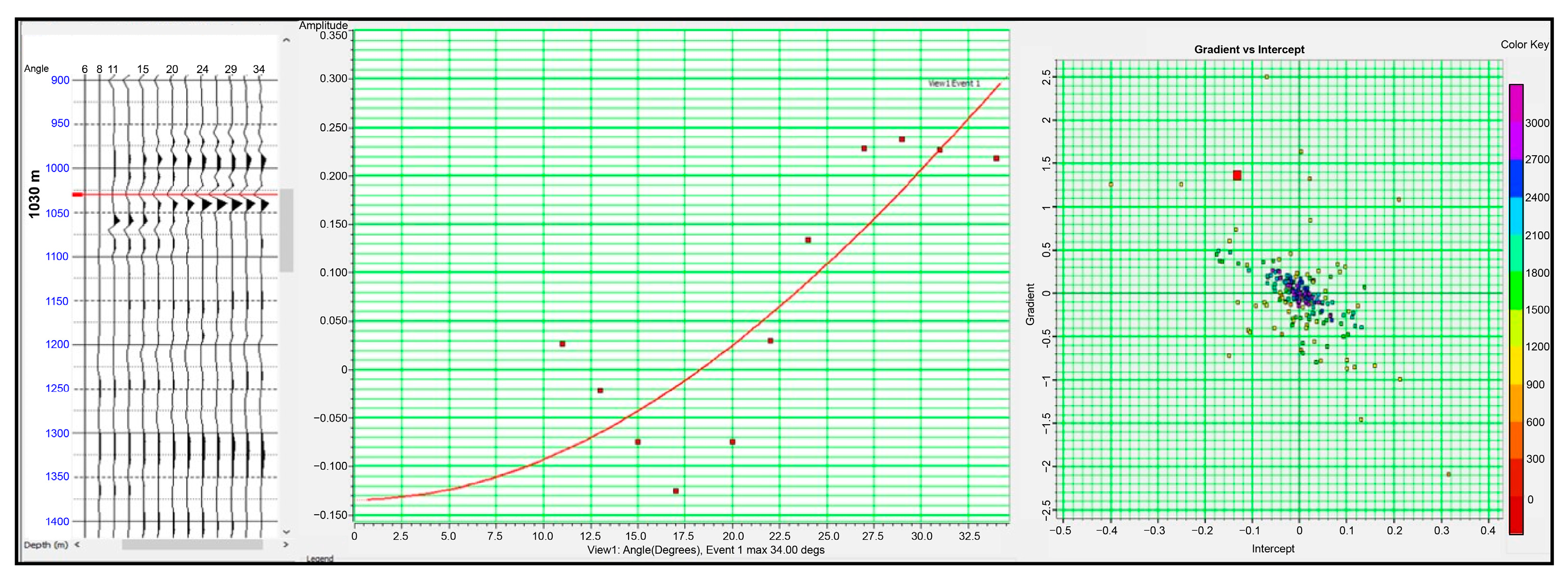
Figure 19.
The AVO gradient curve and associated crossplot of 2014 data. The targeted event, which occurs at 1030 m and is in the second quadrant, exhibits decreasing amplitude with increasing offset. Note a sharp decrease in the strength of the AVO curve compared to 2010 data.
Figure 19.
The AVO gradient curve and associated crossplot of 2014 data. The targeted event, which occurs at 1030 m and is in the second quadrant, exhibits decreasing amplitude with increasing offset. Note a sharp decrease in the strength of the AVO curve compared to 2010 data.

Disclaimer/Publisher’s Note: The statements, opinions and data contained in all publications are solely those of the individual author(s) and contributor(s) and not of MDPI and/or the editor(s). MDPI and/or the editor(s) disclaim responsibility for any injury to people or property resulting from any ideas, methods, instructions or products referred to in the content. |
© 2024 by the authors. Licensee MDPI, Basel, Switzerland. This article is an open access article distributed under the terms and conditions of the Creative Commons Attribution (CC BY) license (https://creativecommons.org/licenses/by/4.0/).
Share and Cite
MDPI and ACS Style
Alam, S.; Knapp, C.; Knapp, J. Three-Dimensional Amplitude versus Offset Analysis for Gas Hydrate Identification at Woolsey Mound: Gulf of Mexico. GeoHazards 2024, 5, 271-285. https://doi.org/10.3390/geohazards5010014
AMA Style
Alam S, Knapp C, Knapp J. Three-Dimensional Amplitude versus Offset Analysis for Gas Hydrate Identification at Woolsey Mound: Gulf of Mexico. GeoHazards. 2024; 5(1):271-285. https://doi.org/10.3390/geohazards5010014
Chicago/Turabian StyleAlam, Saiful, Camelia Knapp, and James Knapp. 2024. "Three-Dimensional Amplitude versus Offset Analysis for Gas Hydrate Identification at Woolsey Mound: Gulf of Mexico" GeoHazards 5, no. 1: 271-285. https://doi.org/10.3390/geohazards5010014