A Review of the Contribution of Satellite Altimetry and Tide Gauge Data to Evaluate Sea Level Trends in the Adriatic Sea within a Mediterranean and Global Context

Abstract

The relatively new sea level satellite altimetry and secular coastal tide gauge data made the reconstruction of sea levels on regional and global scales possible about one century back. Due to better estimations of the Earth’s crustal, glacial, tectonic, and other possible motion biases in tide gauge data, some additional improvements can be expected in sea level reconstructions, analysis, and predictions. A more detailed review of published sea level-related results was conducted for the Eastern Adriatic coast, including the operation of the tide gauge network and data processing, crustal movement estimations, and the establishment of a new reference height system in Croatia, based on five tide gauge sea level data. It was shown that sea level variation and trend-related indicators are spatially homogeneous, especially on a sub-Adriatic scale. The regional Adriatic Sea mean sea level rise rate of +2.6 mm/year for the satellite altimetry era (1993–2019) is less than the global mean sea level (GMSL) rise rate of +3.3 mm/year for the period of 1993–2022. Several empirical methods for GMSL projections and expected IPCC (Intergovernmental Panel on Climate Change) assessments until the end of the 21st century are considered.

1. Introduction

The sea level is one of the most important geophysical variables. It is very sensitive to climate warming and, according to global climate scenarios, its rising/variability is a threat for nearly one billion people living in coastal regions worldwide [1]. At the same time, the sea level is also a key variable in oceanography as a scientific branch of geophysics [2]. The geodetic aspect of the sea level, as a vertical datum, is crucial. For example, the multiannual average of the sea level represents the geodetic normal null (N.N.), i.e., an approximate reference surface of the geoid in sea areas [3,4]. Of equal importance is the hydrographic aspect of the sea level, e.g., a vertical datum called the hydrographic null. The hydrographic null is a geoid surface that is approximately determined by the mean level of lower low waters, and it is related to the security of marine transportation [5].

In situ sea level observations, particularly using conventional tide gauges (TGs), began more than two centuries ago. Initially, such observations served to observe the tide cycle in the sea at ports due to the regulation of marine transportation. Much later, i.e., during the 1980s, the satellite altimetry component started to be operated. Tide gauge stations have been operated since close to the end of the 19th century until today (Figure 1a), when they are unevenly distributed throughout the northern and southern hemispheres, respectively (Figure 1b). Satellite altimetry data have covered well world ocean areas, approximately globally but homogenously, only since 1993 (Figure 2), [6,7]. The sea level was declared as an essential climate variable in 2010 due to the possible significant impact of sea level rise on the environment in coastal areas [8,9]. This aspect is not ignorable in the sense of ‘decision makers’ providing support for the development and maintenance of both hemispheres’ sea level observation networks.

There is a high contribution of satellite geodesy to the overall monitoring of the Earth (e.g., earthquakes, landslides, crustal deformation, etc.). Because of the estimation of the Earth’s crustal, glacial, tectonic, and other possible motion biases in tide gauge data, some additional improvements can be expected in sea level data quality, resulting in improvements in their reconstructions, analysis, and predictions [10,11,12,13].

The present review consists of two core parts; the first is devoted to a regional Adriatic–Mediterranean spatial scale and the second to the global scale.

The first core part of this paper (Section 2) is concentrated on the description of the establishment and operation of the tide gauge network and its data processing for the Eastern Adriatic coast, which mostly belongs to Croatia and includes some parts of neighboring countries [14,15,16,17,18,19]. This region was in the past under the influence of Italy and the Austro-Hungarian Monarchy and thus they share joint TG history. Satellite altimetry principles and calculations of horizontal and vertical crustal motions are described in [3,20,21,22,23,24,25,26,27,28,29,30], respectively. Temporal evolution of sea level in the Eastern Adriatic within a context of the whole Adriatic and Mediterranean seas is discussed [31,32,33,34,35,36]. The second core part (Section 3) is mostly devoted to global-scale sea level trends and variations [37,38,39,40,41,42,43,44,45,46,47,48,49,50,51,52,53]. Semi-empirical versus process-based approaches for projecting future sea level rise is also considered [54,55,56,57,58,59,60,61].

The main goals of this review are to introduce the potential readers to (1) tide gauge network establishment and its data processing standards on the Eastern Adriatic coast; (2) the quality of TG data in the same area in the 20th century; (3) a redefinition of a new geodetic height reference system of Croatia; (4) the results of a comprehensive modelling of Earth’s crustal motion of the Adriatic microplate; (5) the sea level variations and trends in the wider Adriatic Sea area; (6) the long-term sea level trends for the Adriatic Sea after removing crustal motion biases from TG data, (7) the satellite era sea level trends for the Adriatic Sea; (8) the application of Empirical Orthogonal Functions (EOFs) for the reconstruction of the sea level on a regular network, close to globally; (9) 1880–2009 period GMSL rates as well as regional sea level rates; (10) a comparison of the spatial average mean sea level rise rate for the Adriatic Sea for the period satellite altimetry era (1993–2019) by GMSL rise rate for the period (1993–2022); (11) semi-empirical estimations of future sea level projections. The results of goal achievements are also summarized in the conclusion (Section 4).

2. A View on the Regional Sea Level Variations and Trends for the Eastern Adriatic Sea Coast within the Mediterranean Context

2.1. The Mean Sea Level Determination and Its Use for Setting up a New Height Reference System on the Territory of Croatia

2.1.1. The First Published Paper on the Mean Sea Level in Bakar

The area of the Northern and Eastern Adriatic belongs to the areas of the globe with the longest and the densest sea level observations by tide gauges. The oldest TG observations in the region were in Trieste and Venice and they have existed since 1859 and 1871, respectively [62]. The first tide gauge (also referred to as a mareograph) was installed in Croatia in 1929, upon the building of the harbor master’s office in Bakar, a small town located in a bay on the eastern coast of the Adriatic Sea (Figure 3, Figure 4 and Figure A1). That TG is operated by the Geophysical Institute of the University of Zagreb, which is involved in education and research in the fields of meteorology, oceanography, and seismology [32].

Since five years of sea level data for Bakar (1930–1933 and 1935) were available to him, Škreb published the first paper in Croatia on the mean sea level in Bakar in the popular science Croatian journal titled ‘Nature/Priroda’ [64]. The author also discussed tide gauge registration on a tideogram and seiches. According to [64], seiches (a word of French origin) were first observed in the attractive Lake Geneva in Switzerland.

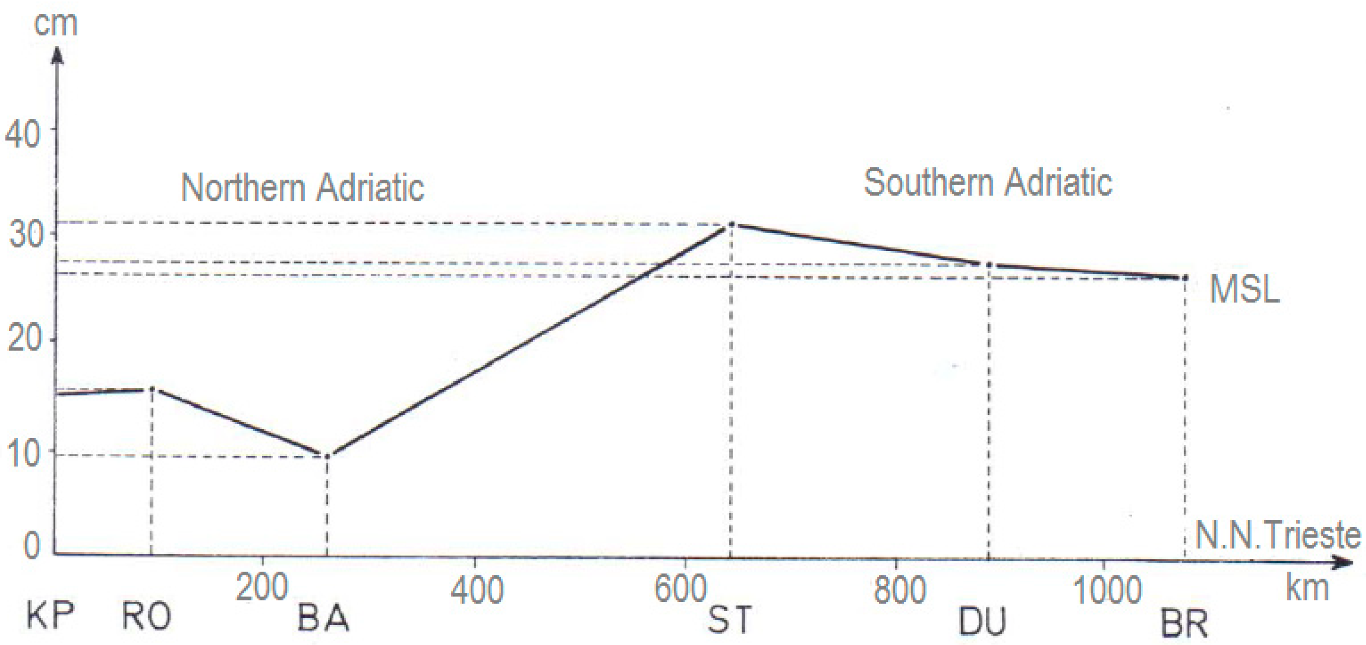
2.1.2. Comparison of the Mean Sea Levels on the Eastern Adriatic Coast

At the beginning of the text in [14], Kasumović said that the mean sea level belongs to a physical (equipotential) reference surface of the geoid, which is equivalent to the citation from [65]: “Any point on the geoid is subject to the same level of gravity and the earth’s geoid is apprximatively set at the mean sea level”. The reference surface of the geoid, which approximately coincides with the mean sea level over sea areas, was chosen to present the reference geodetic vertical datum (geodetic normal null—geodetic N.N.), which is used for determination of the Earth’s crust elevation above that level. By convention, geodetic N.N. has zero absolute elevation. In addition, Kasumović cited the importance of sea level data for ‘early warnings’ on ‘high’ and ‘low’ sea water levels for navigation, especially in coastal areas including ports. The difference between these two extremes can be more than 10 m in some parts of the world.

It was cited in [14] that geodetic N.N. for Trieste, obtained by the tide gauge data for the year 1875, is about +9 cm lower than that for Bakar, obtained on the basis of 7-year tide gauge data for Bakar from the 1930s. The reason for such a difference is an exceptionally low average annual sea level in Trieste for the year 1875.

It has to be noted that v. Sterneck in 1904 [14,66] established, on the basis of the data for 8 years for Trieste (1875–1879 and 1901–1904), that 8-year average sea level is +8.99 cm (approximately +9 cm) higher than the 1-year average for the year 1875 for Trieste, due to the extremely low annual average sea level for the year 1875 for Trieste, which was also mentioned by Kasumović in [14].

Since the year 1954, the Hydrographic Institute of the former Yugoslav Navy has been publishing data on sea level fluctuations according to the registration of all the tide gauges in the former Yugoslav area of the Adriatic (Figure 3) [67,68]. Although all the tide gauges have not been under the management of the cited Hydrographic Institute, the handling of the instruments in the operation and the processing of the sea level data has been carried out according to the same professional principles. Therefore, the published data represent homogenous material on the unevenness of the sea in certain parts of the Adriatic [15].

However, the use of these data for the purpose of comparing the sea level along the Adriatic was not possible, because the water levels of all the tide gauges were counted from different basic levels, abbreviated as TGZ (tide gauge zero) in Figure A1. As the differences between the TGZs of different TGs were not known, it was decided at the Geophysical Institute of the University of Zagreb that they had to be determined within the framework of the International Geophysical Year at that time.

“By knowing these differences, the sea levels of all the tide gauges can be reduced to the basic level of one of them, and in that way, it can be determined whether the mean sea level of the Adriatic is ‘flat’ or not, and if not, what is it”

—Kasumović asked himself in [15].

Jovanović’s findings [16] do not fully support Kasumović’s results on the ‘flatness’ of the mean sea level of the Eastern Adriatic coast, published in [15], probably due to a difference in the length of the time series considered (too short time series were used by Kasumović in his study, i.e., 3 years only). In other words, Jovanović established, on the basis of sea level data for the period 1954–1977, that the local mean sea levels for Koper (+15.00 cm), Rovinj (+15.55 cm), Bakar (+9.88 cm), Split (+31.79), Dubrovnik (+27.60 cm), and Bar (+26.98) were higher than geodetic N.N. for Trieste, based on the sea level data for the year 1875 only [16]. “Corrections” for the three TG stations from the northern Adriatic (rather close to Trieste) were more than two times lower, on average, than those three from the Southern Adriatic (rather far from Trieste). This is shown in Figure 5.

Bilajbegović and Marchesini in 1991 obtained very similar results to those of Jovanović for the mean sea levels for an 18.6-year period (1962.2–1980.8) for the following tide gauges: Koper (+15.24), Rovinj (+15.04), Bakar (+13.83), Split Luka (+31.32), Dubrovnik (+27.72), and Bar (+26.98) [17]. Thus, there is a tendency of stabilization of a higher mean sea level in the Southern Adriatic and a lower mean sea level in the northern part, in relation to N.N. for Trieste for the year 1875. Still, there is no guarantee that all these vertical datums are distributed across the geoid, but instead they are distributed on relatively flat plains in the Southern and Northern Adriatic, respectively. A more accurate answer requires additional research of this topic, e.g., by filtering out the “mean dynamic topography” from the sea level data, whose definition will be introduced in Section 2.2.

2.1.3. A New Reference Height System of the Republic of Croatia

Since the Republic of Croatia became independent after the beginning of the 1990s, significant work has been devoted to the improvement of the existing fundamental height networks inherited from the former Yugoslavia but mostly initiated by the State Geodetic Administration and the Faculty of Geodesy of the University of Zagreb [4]. The origin for the new reference height system of Croatia has been determined by the mean sea levels at five tide gauges along the eastern coast of the Adriatic Sea. Years of mechanical tide gauge installation are cited in brackets after their names, and they have still been operating in a modernized form since the year 2005 [69]: Kopar (1962), Rovinj (1955), Bakar (1930–1938, 1954), Split (1954), and Dubrovnik (1954). The absolute heights of the TG referent benchmarks are 1.8826 m, 4.8377 m, 2.6601 m, 3.3322 m, and 3.6771 m, respectively. Apart from these tide gauges, six fundamental benchmarks, with a very high quality of the underground stabilization, have also been integrated in the height system: Brajkovići, Kostajnica, Knin, Koprivnica, Otočac, and Strizivojna (Figure 6). All the tide gauges which, by highly accurate levelling, are connected with a skeleton of the height system have been continuously observing the sea level for 18.6 years, and the mean sea levels have been determined for the period from the year 1962.2 to the year 1980.8, centered on 1st July 1971, i.e., on the year 1971.5. Computationally determined mean sea levels were transferred to reference benchmarks next to each tide gauge, i.e., the absolute heights of these benchmarks were determined by these mean sea levels.

HRG2009 (HR—international abbreviation of Croatia; G—Geoid; year 2009) geoid solutions for Croatia of ‘very high reliability’ [18,19] are reprinted in Figure 7. According to these results, most geoid surface isohypses are approximately parallel to the Eastern Adriatic coast and thus the mean sea levels are approximately constant for the closest TGs at least. An exception is the southern part of the area where geoid surface isohypse pattern is more complex.

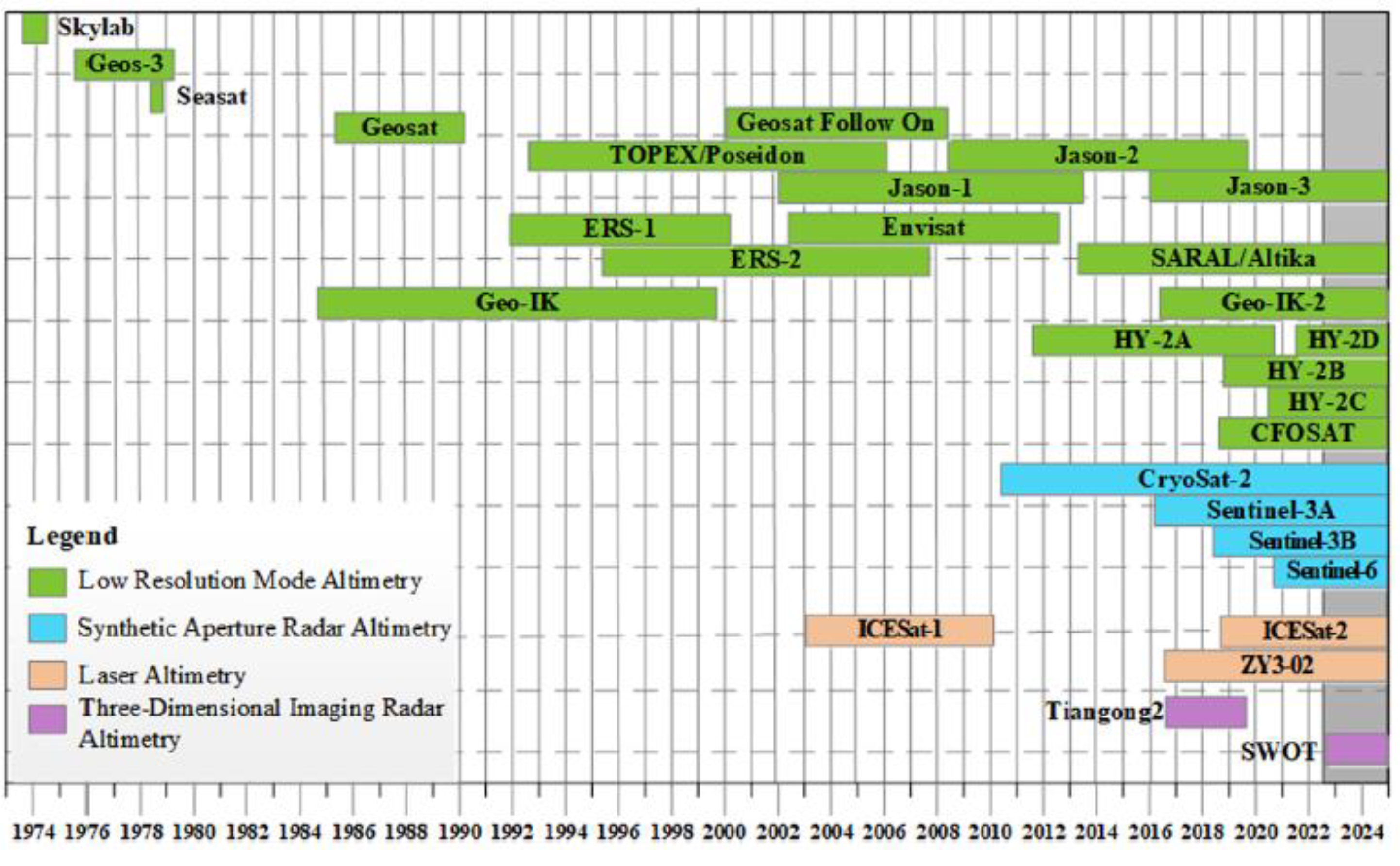
2.2. Satellite Altimetry Principles and an Example of Sea Level Monitoring on the Eastern Adriatic Sea

Satellite altimetry is one of the more recently developed methods of satellite geodesy [3]. The basic concept is rather simple. The satellite serves as a moving platform for a sensor which transmits microwave pulses in the radar frequency domain to the ground and receives the return signals after the reflection from the Earth’s surface. According to [3,70], altitude R (range measurement) of the satellite above the Earth’s surface can be derived as a first approximation from the observed two-way travel time Δt of the radar signal (Figure 8):

R = c (Δt/2)

(1)

where c is the speed of light.

Due to the reflective properties of water, the method is suitable for use over the oceans. A circular area of several kilometers is illuminated at the instantaneous sea surface, the size of which is related to the spatial resolution of the incoming microwave beam. Thus, the observation refers to the mean instantaneous sea surface height, which differs from the geoid height by a separation, $h_d$, referred to as dynamic topography, while $h_g$ (the distance between the reference geoid and ellipsoid surfaces) is referred to as geoid topography (see Figure 8). Height H of the satellite above the global ellipsoid can be derived from an orbit computation with respect to a geocentric reference frame. If additional corrections, shown in Figure 8, such as ocean tide heights ${{\displaystyle h}}_{\tau }$ and atmospheric effects ${{\displaystyle h}}_a$, are at first neglected, the basic simplified altimeter equation is:

$$H={{\displaystyle h}}_g+{{\displaystyle h}}_d+R,$$

(2)

where $h=h_g+h_d$ is the instantaneous sea surface topography. A more detailed satellite sea level observation equation has been considered in [71]. For a description of improved estimations of the mean dynamic topography using satellite altimetry and the tide gauge observation data in coastal areas, please see references [72,73,74].

The mean monthly and annual anomalies of the sea level, referred to as the multiannual averages (1993–2012), for coastal Croatia are shown in Figure 9. Clear seasonal variations are visible in monthly values with an amplitude of around 10 cm, while multiannual variations and the positive trend of about 2 mm/year are visible in annual mean sea level values.

2.3. Determination of Vertical Motion of the Adriatic Crustal Microplate

The issue of ‘noise’ in TG records produced by non-eustatic factors, such as tectonic crustal motions and glacial isostatic adjustment (GIA), was recognized in the 1980s. In the acknowledgments of their esteemed book on the topic, Emery and Aubrey in 1991 [25] do not provide a very optimistic conclusion: “In essence, we have concluded that the ‘noise’ in the TGs’ records is produced by tectonic crustal motions and both meteorological and oceanographycal factors so it obscures any signal of the increase of eustatic sea level and that the tide-gauge records are more useful for learning about plate tectonics than about the effects of the greenhouse warming of the atmosphere, glaciers, and ocean water”. Much more optimistic results on the issue, for some parts of the globe, were published a few decades later, e.g., [22,23,24,26].

2.3.1. Application of Geodetic Modelling and GPS (Global Position System)/GNSS (Global Navigation Satellite System) Observations for Determination of Crustal Motions

A number of recently published scientific papers addressed the issue of noise in TG sea level data on the eastern Adriatic coast, which is a tectonically active area. Some of these results have been provided in this review.

Marjanović et al. in [21] described the application of geodetic modelling and GPS measurements for the determination of horizontal and vertical motions on the Adriatic microplate. The measurements were carried out in the period between 1994 and 2005 within the frame of the 21 measuring GPS campaigns organized in the research area. During the planning of the CroDyn Project [75], five GPS stations were installed near the existing tide gauges on the eastern Adriatic coast, which were included in GPS campaign and data processing (

Table 1. Co-locations of the tide gauges and GPS points on the eastern Adriatic Sea coast of Croatia (the first column). The number of years of a particular TG in operation (the second column), the number of GPS sessions (the third column), and the average vertical motion Vu (mm/year) of GPS and TG points during campaign 1994–2005 (after [21]).

TG/GPS Stations	TG [Number of Years]	GPS [Number of Sessions]	Vu [mm/year]
Bakar	62	17	−1.2
Dubrovnik	47	17	−1.2
Rovinj	48	19	−0.4
Split	50	17	−2.1
Zadar	10	11	−0.9

). The processing of GPS data, as well as the computation of the coordinates of the chosen crustal points and their velocities, was performed by “Bernes GPS Software Ver. 5.0” [76], based on 140 daily solutions. The international global navigation satellite systems service (IGS) point Graz (Austria) was used for datum definition for coordinates, as well as for velocities.

The trends of sea level changes and computed ellipsoidal heights for all the tide gauges and GPS points, as well as signs of determined vertical (Vu) velocities (Table 1), show their relative motions in the vertical sense, the rise of the sea level or descending of the coast. Also, the values of correlation coefficients between two time series are approximately −1 (e.g., for Bakar, Figure 10 and Figure 11).

Please note that on 5 September 1996 at 22:44 local time (CEST, 20:44 UTC), Southern Croatia was hit by a strong earthquake of magnitude 6.0. The epicentre was near the eastern coastline of the Adriatic Sea, close to the town of Slano about 30 km northwest of Dubrovnik. That could be the reason why GPS heights started to decrease at TG/GPS in Bakar since 1996, although they rose over the previous two years, perhaps due to an unstable pillar in Bakar which is sensitive to earthquakes [25,77] (Figure 11).

These results from [21] could be compared with similar studies in the area.

Thus, a comparison of horizontal velocities between these two solutions (1996–1998 and 1994–1998) by Altmer et al. [77] indicates that the motion of the Bakar station, number 2 in Figure 12, exhibits a different magnitude (velocity) and direction for each solution. The authors of [77] assumed that the motion for this station is local due to unstable pillar. However, at the 0.95 confidence level, the vertical velocities for most of the stations are not significant, and hence, they were not discussed in [77].

GPS/GNSS observations from 83 stations all over Croatia performed for almost 20 years (1994–2013) were collected by Pavasović et al. in [75] and processed with the Bernese Software version 5.0 [76] to obtain a unique database of crustal velocities. The results are presented in Figure 13. Horizontal crustal motions are dominant but there are spatially positive motions (uplift) greater than 0°, 20°, 30°, and 60°; spatially negative motions (descending) are greater than 0° or −30°, especially along the Croatian coastline. There are some matching velocities described in [21,75], respectively.

2.3.2. Application of Satellite Altimetry and TG Sea Level Data for Estimation of Absolute Crustal Motion

Cazenave et al. [27] calculated sea level differences TOPEX/Poseidon (T/P) minus tide gauge (TG) for the period 1993–1997 at 53 selected tide gauge sites, which is subsequently referred to as a ‘classical approach’. A comparison of these sea level differences with vertical crustal motions derived from space geodesy systems at six co-located sites shows reasonable consistency. At other sites, showing large trends, further research is required to explain the observations.

Kuo et al. [28] presented a new ‘advanced approach’ of combining rather short satellite altimetry sea level data and much longer tide gauge data by constraint equations to obtain improved estimates of absolute (or geocentric) vertical crustal motion at tide gauges within a semi-enclosed Baltic Sea region. For illustration, they combined TOPEX/Poseidon altimetry data (1992–2001) and 25 long-term (>40 years) tide gauge records around the Baltic Sea, where crustal deformation is dominated by glacial isostatic adjustment (GIA). A comparison of estimated vertical motion from 1 to 11 mm/year, with independent solutions from 10 co-located GPS sites, shows a difference of 0.2 ± 0.9 mm/year, which verifies the robustness of the procedure.

Wõppelmann et al. [29] applied the same procedure to some semi-enclosed parts of the Mediterranean Sea, including the eastern coast of Croatia and a part of the open Atlantic Ocean (Figure 14), following Kuo et al.’s [28] improved estimation of vertical crustal motion for the semi-enclosed Baltic Sea. The results have been compared with Cazenave et al.’s [27] approach and GIA model results, which have been provided for comparison and easier interpretation of total vertical land movements, especially in the areas where GIA’s results are dominant and refer to longer periods [29,78]. The results are presented in

Table 2. Geocentric vertical land motions (mm/year) at the selected Permanent Service for Mean Sea Level (PSMSL) TG stations and satellite altimetry data, either from the classic or the advanced approach (after [29]).

Station (PSMSL)	Altimeter—TG Classical Approach (1992–2010)	Altimeter—TG This study/Advanced Approach (All Data)	GPS (ULR Solution)	GIA (SELEN)
Santander I	−1.62 ± 0.43	0.91 ± 0.34	−0.09 ± 0.23	−0.55 ± 0.26
La Coruña I	0.19 ± 0.60	0.73 ± 0.33	−2.19 ± 1.82	−0.80 ± 0.26
Vigo	3.64 ± 0.64	0.57 ± 0.33	-	−0.70 ± 0.31
Cascai	0.43 ± 0.66	-	0.18 ± 0.16	−0.62 ± 0.22
Marselle	−0.23 ± 0.45	0.17 ± 0.20	−0.04 ± 0.25	−0.59 ± 0.19
Venezia (PDS—Punta Della Salute)	−2.03 ± 1.32	−1.22 ± 0.19	1.40 ± 3.06	−0.43 ± 0.19
Trieste	−0.31 ± 0.39	0.30 ± 0.19	-	−0.41 ± 0.19
Rovinj	1.95 ± 0.42	0.75 ± 0.19	-	−0.46 ± 0.20
Bakar	0.03 ± 0.50	0.43 ± 0.18	-	−0.45 ± 0.20
Split Marjan	−0.44 ± 0.44	0.61 ± 0.18	-	−0.58 ± 0.20
Split Gradska Luka	−0.69 ± 0.45	0.70 ± 0.18	-	−0.57 ± 0.20
Dubrovnik	−0.50 ± 0.38	0.32 ± 0.18	−0.92 ± 0.31	−0.60 ± 0.17
Katakolon	0.63 ± 0.47	0.06 ± 0.21	-	−0.84 ± 0.23
Thessaloniki	−1.38 ± 0.47	−1.96 ± 0.25	-	−0.63 ± 0.22
Alexandroupolis	0.01 ± 0.47	0.02 ± 0.28	-	−0.64 ± 0.20
Leros	3.63 ± 0.51	1.28 ± 0.35	-	−0.80 ± 0.19
Alexandria	0.37 ± 0.70	−0.40 ± 0.23	−0.10 ± 0.50	−0.51 ± 0.07

. Vertical crustal motions for TG stations on the eastern Adriatic coast seem spatially homogeneous from Trieste in the north to Dubrovnik in the south. We will return to this matter in the following section, Section 2.4, where sea level trends and variations will be considered.

2.4. Some Studies of Sea Level Temporal Evolution According to Tide Gauge Observations on the Eastern Adriatic Coast in the Adriatic–Mediterranean Context

2.4.1. Sea Level Analysis Based on Geomorphological Approach and TG Data

In a review [31] by Surić, an interdisciplinary approach to temporal evolution of sea level on the Eastern Adriatic coast has been applied. A rocky karstified coast, low tidal range, indented shoreline with numerous islands, diverse coastal biocenoses, abundant paleontological, archaeological, and historical evidence, relatively dense tide gauge stations, and developing GPS network—all of these facts provide optimal prerequisites for the sea level change studies on the Croatian coast of the Adriatic Sea. Through various methodological approaches, including geomorphological, biostratigraphical, archaeological/historical, mareographic, geodetic, and radiometric approaches, most of these facilities have been used in order to reconstruct relative sea and land motions on the eastern Adriatic coast, but additional efforts still have to be made for further improvement of the existing knowledge on sea level variations and trends in the area considered. The authors of this review think that the hydrology of eastern Adriatic islands and the hinterland could improve that knowledge too [79]. There is an idea to make a clustering of precipitation anomaly fields on eastern Adriatic Sea islands and the hinterland on the monthly scale for the period 1961–2018, then, using such clustering, examine the connection with river discharge and sea level anomalies for the same region and time scale, including macroscale atmospheric circulation fields for the wider Northern Atlantic, like sea level atmospheric pressure or absolute topography (AT) anomalies of standard surfaces of constant air pressure, like AT 1000 hPa and AT 500 hPa [80].

The monograph [32] of the Geophysical Institute in Zagreb (Croatia), by Orlić (ed.), provides a very concise description of temporal changes of sea level on the eastern Adriatic coast. Thus, it was cited that Orlić and M. Pasarić in [33,34] have established that the sea level in the Adriatic was rising in reference to the land, but that in the mid-20th century, this increase slowed down, which was, according to Tsimplis [81], an indicator of deep water salinity and temperature change in the Mediterranean area. Orlić and M. Pasarić in [33,34] have also noticed that, in addition to changing trends, well-defined quasi-periodic oscillations (from 10 to 20 years) are pronounced in the Adriatic. They presumed that understanding such one-decadal and two-decadal oscillations is a necessary prerequisite for their elimination from the time series and hence a more reliable determination of the trends.

Tsimplis and Josey [82] said that the observed reduction in Mediterranean Sea level has occurred at the same time as rising levels elsewhere are expected to accelerate because of anthropogenic climate change (see [83]). The processes which they have discussed raise the worrying possibility that the anthropogenic increase in sea level in the Mediterranean is being masked by the effects of natural atmospheric variability. The situation is further complicated by the possibility that the frequency of occupation of different atmospheric states has been altered as a result of climate change (see [84]). Tsimplis et al. [62] estimated that sea level trends in the Adriatic Sea show variability in time and space. Spatial variability was assessed by estimating the differential trends in reference to Trieste. For many of the stations, the differential trends become smaller than error bars. That indicates that land, atmosphere, and oceanic contributions are rather uniform over the basin. The observed trends for longer records differ for the periods before 1960 and after 1960. They tried partly to explain this by atmospheric forcing, estimated as −0.8 mm/year for the period 1960–2000.

Following their previous research, Orlić and M. Pasarić obtained valuable results, published in [35], which are partly presented in Figure 15. They concluded that there are some indications that over the last twenty years or so, the rate of the sea level rise considerably increased in the Black Sea and thus surpassed the rate in the Atlantic, while in the West Mediterranean and in the Adriatic, it became similar to the rate in the Atlantic.

Vilibić et al., in a comprehensive review paper on the sea level in the Adriatic Sea [36], provide an extensive review of the best available knowledge dealing with the sea level changes in the Adriatic, including the generation of the destructive tsunami-like waves.

2.4.2. Examples of Sea Level Trend Analysis Using Both Satellite Altimetry and Tide Gauge Data

Following vertical land motion data from Table 2, Wõppelmann et al. [29] determined new sea level trend velocities (mm/year) presented in

Table 3. Rates of the sea level changes from the tide gauge records and corrected by the land motions from different solutions. Combination of the satellite altimetry and the tide gauge data using classical and advanced approach, GPS and GIA. In columns 2–6, units are in mm/year. Please note that spatially homogenous results for “advanced altimeter—TG” results for the Eastern Adriatic coast are highlighted (after [29]).

Station (PSMSL)	No Corrections	Altimeter—TG Classic	Altimeter—TG Advanced	GPS Corrected (URL Solution)	GIA Corrected (SELEN)
Santander I	2.07 ± 0.13	0.4 ±5 0.45	2.98 ± 0.36	1.97 ± 0.26	1.52 ± 0.29
La Coruña I	2.21 ± 0.14	2.40 ± 0.62	2.94 ± 0.36	0.02 ±1.83	1.42 ± 0.30
Vigo	2.35 ± 0.14	5.99 ± 0.66	2.92 ± 0.36	-	1.65 ± 0.34
Cascai	1.29 ± 0.04	1.79 ± 0.66	-	1.14 ± 0.19	0.35 ± 0.24
Marselle	1.22 ± 0.04	0.99 ± 0.45	1.39 ± 0.20	1.18 ± 0.25	0.63 ± 0.19
Venezia (PDS)	2.45 ± 0.09	0.42 ±1.32	1.24 ± 0.21	3.85 ± 0.60	2.02 ± 0.21
Trieste	1.28 ± 0.07	0.97 ± 0.40	1.58 ± 0.20	-	0.87 ± 0.20
Rovinj	0.53 ± 0.17	2.48 ± 0.45	1.27 ± 0.25	-	0.07 ± 0.26
Bakar	1.03 ± 0.12	1.06 ± 0.51	1.46 ± 0.22	-	0.46 ± 0.26
Split Marjan	0.64 ± 0.16	0.20 ± 0.47	1.25 ± 0.24	-	0.06 ± 0.26
Split Gradska Luka	0.64 ± 0.16	−0.05 ± 0.48	1.33 ± 0.24	-	0.06 ± 0.26
Dubrovnik	1.02 ± 0.16	0.52 ± 0.41	1.33 ± 0.24	0.10 ± 0.35	0.42 ± 0.23
Katakolon	1.97 ± 0.22	2.60 ± 0.52	2.03 ± 0.30	-	1.13 ± 0.32
Thessaloniki	3.88 ± 0.24	2.50 ± 0.53	1.93 ± 0.34	-	3.26 ± 0.33
Alexandroupolis	2.05 ± 0.27	2.06 ± 0.54	2.07 ± 0.39	-	1.42 ± 0.34
Leros	0.93 ± 0.24	4.56 ± 0.56	2.21 ± 0.42	-	0.14 ± 0.31
Alexandria	1.81 ± 0.12	2.18 ± 0.74	1.41 ± 0.29	1.64 ± 0.51	1.23 ±0.14

. Lengths of the most TG time series for the eastern Adriatic area were (in years) Trieste at 106 (1905–2010), Rovinj at 54 (1955–2008), Bakar at 79 (1930–2008), Split Marjan at 57 (1952–2008), Split G. Luka at 54 (1954–2008), and Dubrovnik at 53 (1956–2008). The most spatially homogeneous results are for the case of satellite altimetry and TG records’ combination using an advanced approach (Table 3, yellow color).

A step forward was made by De Biasio et al. [30], who consider a similar analysis for six TGs for the northeastern Adriatic coast, three for Italy, and three for Croatia. At a regional scale of the Adriatic Sea, represented with six TGs, the average sea level rate is 2.43 mm/year for the period (1974–2018); see

Table 4. Rates of the absolute sea level change from TG records over whole record (1974–2018), corrected for geocentric vertical land motions (VLMs) estimated by the linear inverse problem (LIP), including covariance (LIP_cov), where $\dot{\varsigma }$ is relative sea level rates during TG life time. All data are in mm/year. Please note that VEPTF is a TG near Venice (after [30]).

Location	$\dot{\mathit{\varsigma }}-\mathbf{LIPcov}$
VENEZIA *	2.33 ± 0.83
VEPTF	2.37 ± 0.86
TRIESTE *	2.71 ± 0.75
ROVINJ	2.29 ± 0.80
SPLIT *	2.57 ± 0.74
DUBROVNIK	2.28 ± 0.74
Pooled mean	2.43 ± 0.80
Sample mean	2.43 ± 0.18

* Asterisk near the TG name indicates that the SL record has been reconstructed from different sources.

. The TOPEX/Poseidon mission suffered from an observation bias or drift of the TOPEX-A instrument during the period 1993–1998. The current bias has been estimated through a sea level budget closure approach and comparison with tide gauge data. In the last case, we need to be careful if both satellite altimetry and tide gauge data are simultaneously biased in terms of observation.

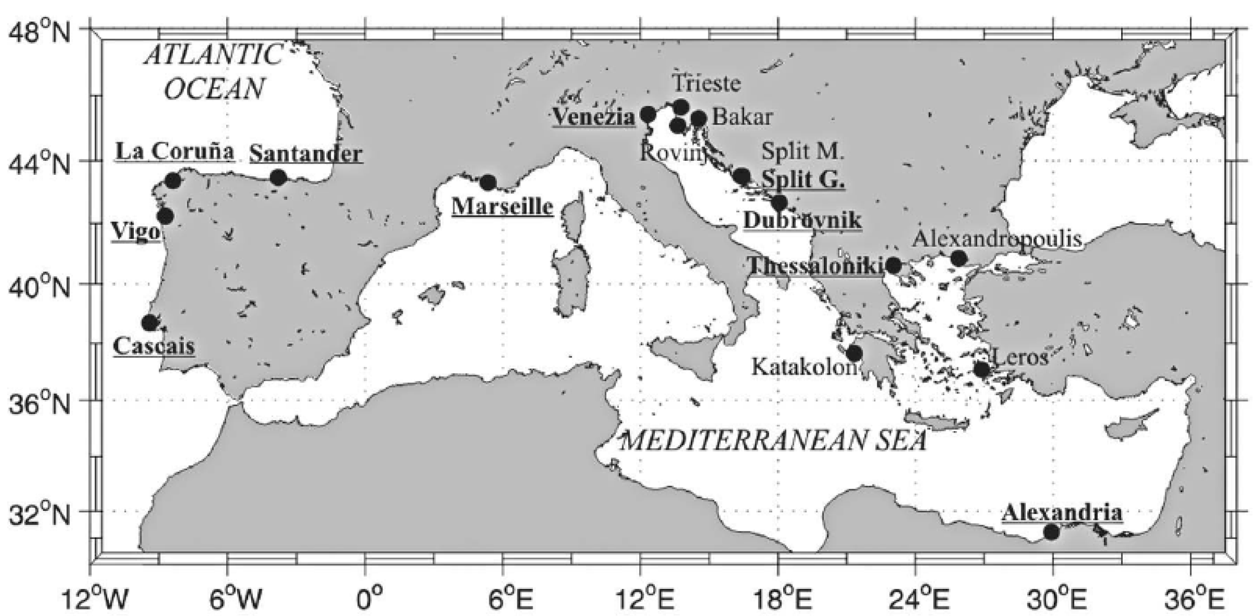
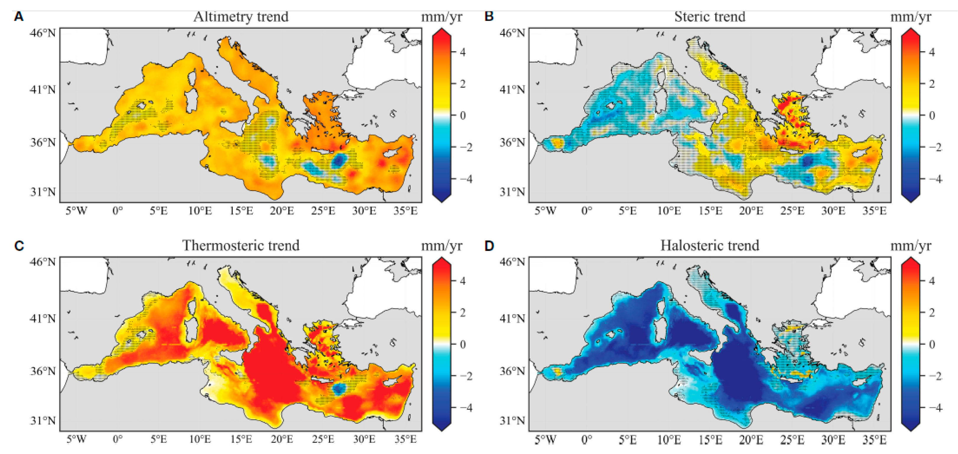
2.4.3. Spatial and Temporal Variability of Sea Level Trends in the Mediterranean Sea for the Period 1993–2019

Meli et al. [85] considered the spatial variability of sea level change rates in the semi-enclosed Mediterranean Sea. They studied sea level trends for the 1993–2019 period using satellite altimetry sea level gridded data. Sea water temperature and salinity on vertical profiles in the sea were taken from the archive of oceanographic reanalysis data. These data were used to calculate thermosteric and halosteric effects on the sea level trends.

Long-term linear trends of total sea level change at the sub-basin scale confirm spatial variability of sea level trends as a consequence of local processes. Sea level trend can be considerably influenced at a regional scale by the contribution of glacial isostatic adjustment (GIA), the gravitational, rotational, and deformation (GRD) effects, and the dynamic component of sea level, induced by the lateral mass transport. In the Mediterranean Sea, the GIA contribution is relatively small (−0.3 mm/year), while the GRD effects contributed about 1.5 ± 0.2 mm/year during the period 2000–2018. All these terms are “non-steric effects”. The values +1.8 mm/year, +2.1 mm/year, and +2.5 mm/year are observed for the Western Mediterranean, the Southern Central Mediterranean, and the Tyrrhenian Sea, respectively. Higher trends of +2.6 mm/year are observed for the Adriatic and the Levant, while +3.1 mm/year was for the Aegean Sea. Conversely, the trends for the Ionian Sea of +1.6 mm/year and Southern Crete of +0.3 mm/year, respectively, are not significant (Figure 16). There is a clear indication that the non-steric effects over the Mediterranean are dominant, except in the Levant and the Aegean sub-basins, where steric effects explain the majority of the sea level trends (Figure 16B–D). The main changes in sea level trends were detected around 1997, 2006, 2010, and 2016 in connection with the North Ionian Gyre reversal episodes, which changed the thermohaline properties and water mass redistribution over the sub-basin. It has to be emphasized that the higher trend of +2.6 mm/year for the Adriatic Sea is fully supported by tide gauge sea level observations, corrected for vertical crustal motion with a high confidentiality in the case of the so-called advanced approach, on the Adriatic coast for the period 1974–2018, presented in Table 4 in the last two rows of the second column.

Although thermosteric trends are often higher than the total sea level trends in the Mediterranean Sea, their overall contribution to the steric component is strongly influenced and lowered by the negative contribution of the halosteric effect. This opposite effect is the direct outcome of the progressive regional increase in water temperature and salinity. This fact highlights the extent to which the halosteric effect is influential within semi-enclosed basins at mid-latitudes, as opposed to the global oceans, where the thermosteric effect represents the dominant driver of steric component trend and variability (see Section 3.4 and [60]).

Orlić et al., in [86], considered trends of sea water temperature and salinity for the period 1952–2010 in a spatial vertical cross-section in the Central Adriatic (the results are presented in two figures on page 490 of the book [86]). Although the considered period is more than twice as long as the satellite altimetry era, considered in the above study by Meli et al. [85], the conclusion was that the time series needs to be 60–80 years long for the calculation of stable secular trends, as otherwise, the trends can be just a part of long-term oscillations. For more details, please see also [87]. Even in the case that time series are long enough, say more than 100 years, the comparison between trends in the local- and the global-scale sea levels needs to be carefully made because, even at such a secular time scale, some local influences, such as air pressure and wind, can be more emphasized at the local than at the global scale [2].

3. A View on Global Sea Level Trends and Variations

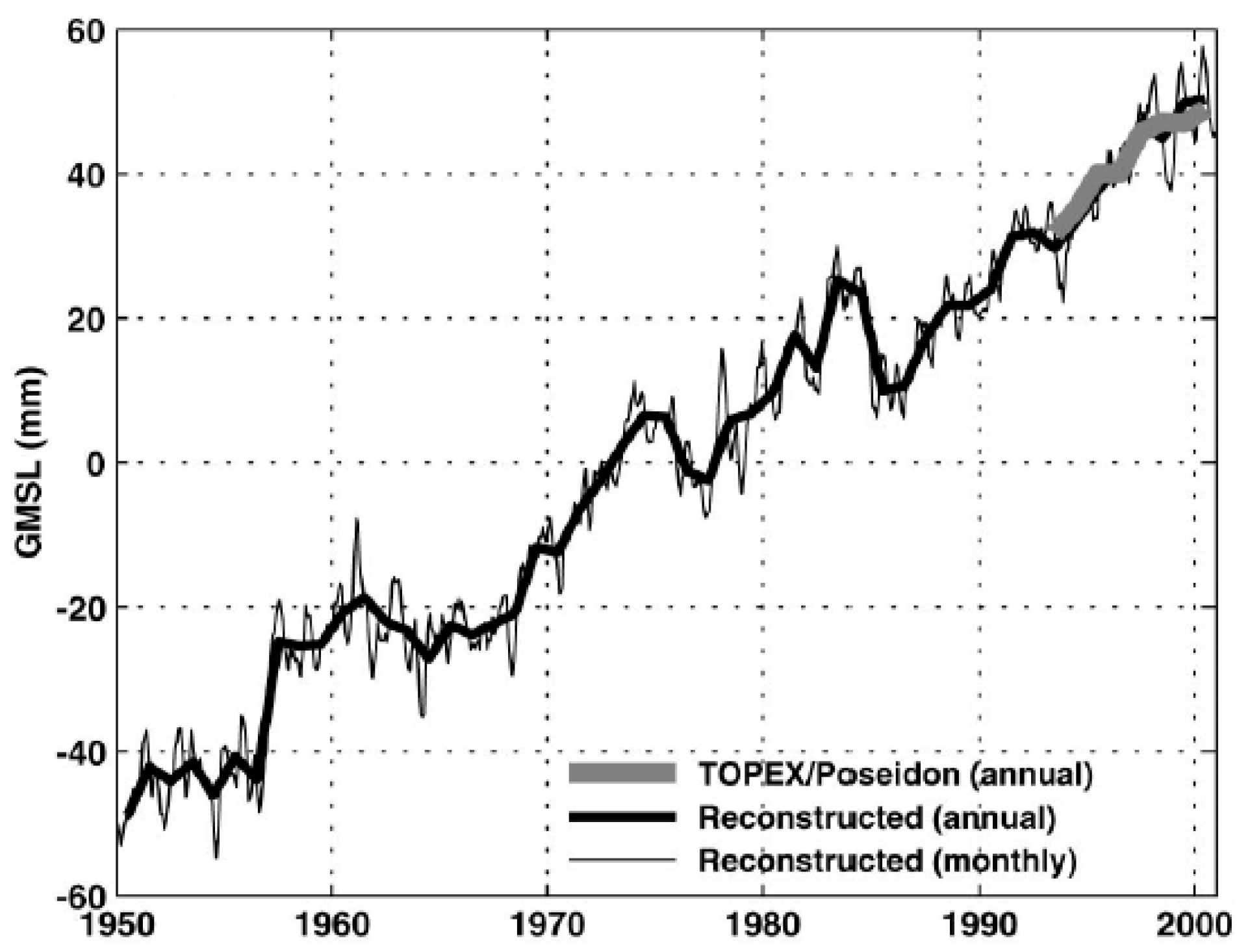
3.1. Estimates of the Regional and Global Sea Level Rise over the 1950–2000 Period

A series of valuable scientific papers on the topic of sea level variations and trends was published during the end of the 20th century and in beginning of the 21st century, e.g., [38], expressing joint use of complementary TG and satellite altimetry sea level observation data.

The approach used in [39] relies on resolving large-scale sea level trend variability by using as many tide gauge records as possible to estimate the global distribution of sea level for each month/year between 1950 and 2000. The authors used the available satellite altimetry data to estimate the global covariance structure as expressed in empirical orthogonal functions (EOFs). Then they estimated the amplitudes of M (= 10, 20…) leading EOFs by using the relatively sparse but longer tide gauge records. It was assumed that the global covariance structure is not significantly dependent on time. The authors of this review recommend to potential readers references [41,42,43,44] on EOFs and their applications in geophysics, especially in meteorology and oceanography.

Monthly and yearly average global sea level changes are presented in Figure 17. Due to decadal variations in mean global sea level, it was not possible to determine any temporal variations in the rate of sea level rise between 1950 and 2000, i.e., estimate the GMSL acceleration. The regional distribution of sea level rise rates between January 1950 and December 2000 is presented in Figure 18.

The authors of [39] emphasized that the results highlight the value of the Global Sea Level Observing System (GLOSS) tide gauge network in the satellite altimetry era. Computed average rate of GMSL rise is 1.8 ± 0.3 mm/year for the period 1950–2000. The major sources of uncertainty in the results are inadequate geographical distribution of tide gauges, particularly in the Southern Hemisphere, inadequate information on various geophysical signatures in the tide gauge data (glacial isostatic adjustment and tectonic activity), and the short satellite altimetry record used to estimate global sea level covariance functions.

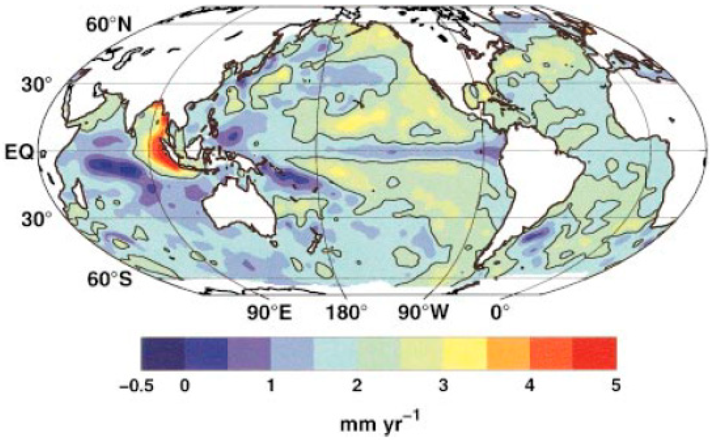
3.2. Sea Level Rise from the Late 19th to the Early 21st Century

Church and White [6] have extended the 1950–2000 period to 1870–2001 and, using 10-year smoothing, estimated a linear sea level rise of 1.7 ± 0.3 mm/year and an acceleration of sea level rise of 0.013 ± 0.006 mm/year². They concluded that if this acceleration remains constant, then the 1990-to-2100 rise would range from 280 to 340 mm, which is consistent with climate change simulations and climate projections of sea level for the period 1990–2100 in the IPCC Third Assessment Report [50].

Church and White [40] have continued to contribute to the understanding of the GMSL trend and variations. They estimated the rise of the GMSL from satellite altimetry data for the 1993–2009 period and from coastal and island TG by EOF-reconstructed sea level observations for the 1880–2009 period. The GMSL time series (Figure 19) are not significantly different from their earlier results [6]. The total GMSL rise from January 1880 to December 2009 is about 210 mm over the 130 years. The trend over this period, not weighted by the uncertainty estimates, is 1.5 mm/year.

There is considerable variability in the rate of GMSL rise during the twentieth century, but there has been a statistically significant acceleration since 1880 and 1900 of 0.009 ± 0.003 mm/year² and 0.009 ± 0.004 mm/year², respectively. Since the start of the altimeter record in 1993, global average sea level rose at the rate near the upper end of the sea level projections of the IPCC Third and Fourth Assessment Reports [54,55].

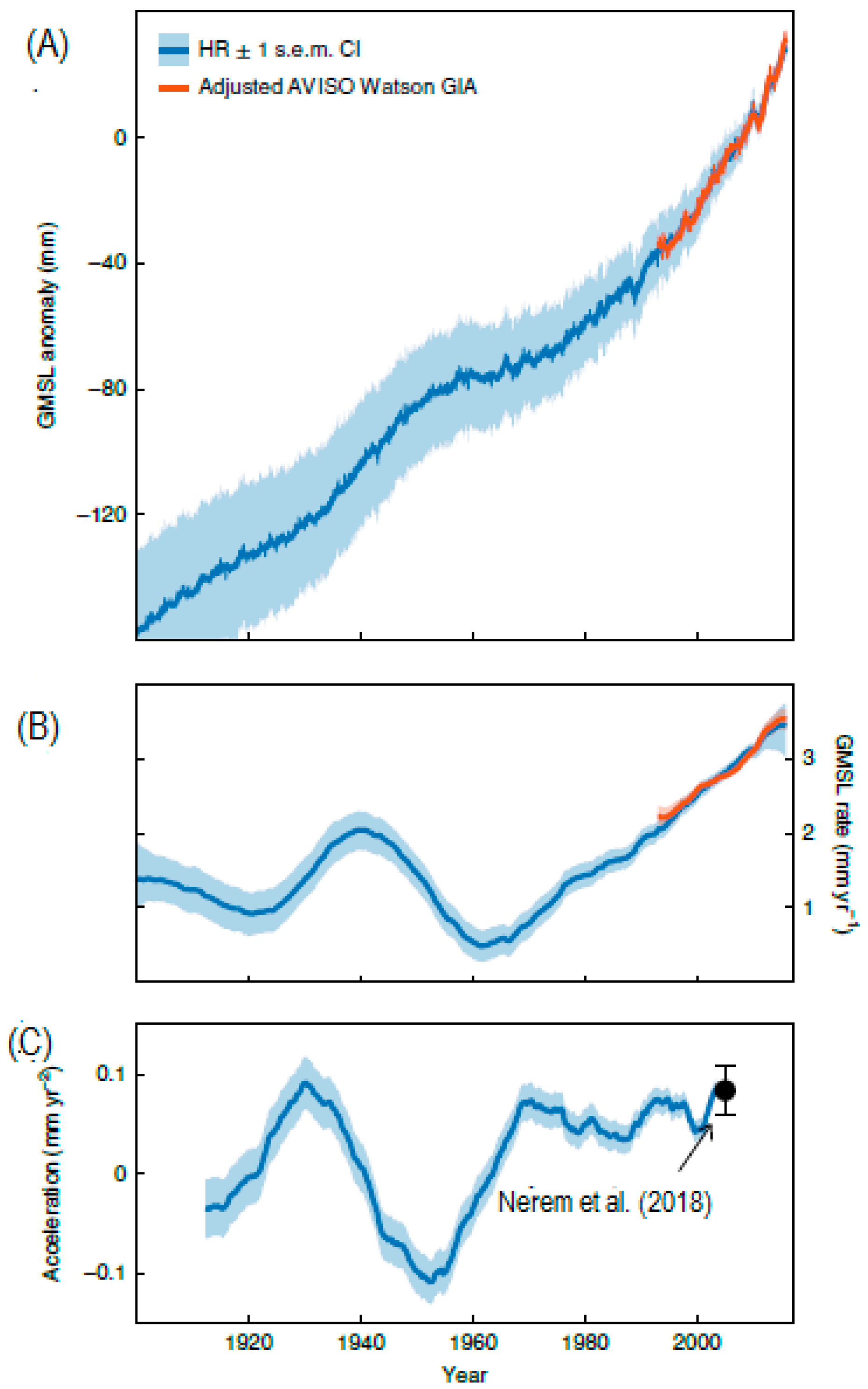
3.3. Persistent Acceleration in Global Sea Level Rise since 1960

As cited in the introductory section of this review, Dangendorf et al. [46] tried to understand whether the recent high sea level rates from the satellite altimetry era area part of a longer-term acceleration. Neither of the techniques, KS (Kalman Smoother) or RSOI (Reduced Space Optimal Interpolation), described more comprehensively in [46], are able to reconstruct the full spectrum of global and regional sea level changes. This contributes to large differences between individual reconstructions before the 1970s and therefore hampers placing the recent acceleration into the historical context of the 20th century. Dangendorf et al. [46] combined the low-frequency sea level information from the KS with the high-frequency information from RSOI reconstructions to generate a hybrid reconstruction (HR) of global and regional sea level during 1900–2015, which uses the two techniques only on those time scales (frequencies) where KS and RSOI reconstruction techniques perform the best, respectively.

The GMSL from the HR (after removing the GIA signal) over the entire period of 1900–2015 is characterized by an average trend of approximately 1.6 ± 0.4 mm/year (Figure 20A), characterized by a considerable multidecadal variability (Figure 20B). During the satellite period, the GMSL rate increased from 1993 (2.1 ± 0.1 mm/year) to 2015 (3.4 ± 0.3 mm/year). This is qualitatively consistent with the drift-corrected altimeter record from AVISO (Archiving, Validation and Interpretation of Satellite Oceanographic data) and estimates from [88] obtained with different statistical methods. According to the results presented in Figure 20C, it was concluded that persistent acceleration of the GMSL rise started in the 1960s and has lasted until the present moment. Similar high acceleration in the period characterized by strong mostly natural warming in the higher latitudes of the Northern Hemisphere, appeared in the1930s, caused by prevailing natural forces.

The authors of this review suggest a comparison of the previous Figure 20B with Figure 21, showing global 60-month average near-surface temperature for 1850–2020, published on the Copernicus portal for the Copernicus programme on climate change. It seems that there could be a significant correlation between the cited global variables. Near the end of the 1930s, average near-surface temperature for the Northern Hemisphere reached a maximum in the period 1890–1960 [89,90].

3.4. Recent Achievements in Satellite Altimetry Era

Cazaneve et al. [49] comprehensively explained the ‘establishment’ of 756 ‘virtual’ altimetry stations close to the coastlines across the globe, within 20 km of the coast (Figure 22), due to about 30 years of continuous satellite altimetry observation of sea level and the specific procedure of satellite altimetry data assimilation. ‘New’ information on sea level change in the coastal zone across the world has become available. Cazaneve et al. [49] tested estimated values for monitoring of regional and global sea level for the satellite altimetry period of 1993–2019. The results showed acceptable matches with ‘regular’ satellite sea level estimations.

Cazaneve et al. [52] reviewed the contemporary sea level changes from the global to the local scale. The first results are presented in Figure 23. The whole period was divided into three linear sea level rise sub-periods: January 1993–December 2002 (rate 2.27 mm/year), January 2003–December 2012 (rate 3.29), and January 2013–March 2022 (rate 4.68 mm/year). The average GMSL rise rate is 3.33 ± 0.33 mm/year for the period January 1993–March 2022. An acceleration in GMSL rise rates of about 0.11 ± 0.01 mm/year² was confirmed.

A global coverage of altimetry missions has enabled estimates of the regional rates of sea level changes. In most regions, positive values of sea level rise rates have been shown (Figure 24 and [52]), while in some areas, the rate of the rise exceeds the 3.33 mm/year global average, which is also evident from Figure 24, From this figure, it is visible that the most extreme anomalies of sea level trends are to the east of Japan, in a range from about −10 mm/year to +10 mm/year relative to the global average. It is very likely that, to a great extent, it is a consequence of significant earthquake impacts on crustal motions. One of the best examples of earthquake crustal motion impact on the tide gauges is that at Nezugaseki (west coast of Honshu Island in Japan), showing considerable and submergence along the coast, generally dominated by emergence. That was impacted by Niigata earthquake of 16 June 1964, whose epicenter was 40 km away, when the mean sea level at Nezugaseki of 113.3 cm changed by +13.4 cm immediately after the earthquake [25]. This is a typical example of a “coseismic” event. However, since tsunami waves appeared in earthquake-prone areas, such as the Mediterranean Sea, a tsunami early warning system has been established on the Island of Crete in the Eastern Mediterranean basin [91].

The sea level budget is more accurate over the 2005–present time span because of the use of GRACE space gravimetry to directly estimate the ocean mass increase rather than individual mass components. For the period 2005–2016, Horwath et al. [53] estimated the thermal expansion and the ocean mass contributions to 34% and 66%, respectively, with the total land ice contributing approximately 55% (Figure 25). See also [2,92].

3.5. Semi-Empirical versus Process-Based Approaches to Projecting Future Sea Level Rise

Since process-based physical models have not yet sufficiently matured, until the second decade of the 21st century, semi-empirical models for estimation rate of mean global sea level (MGSL) rise were provided as a pragmatic alternative to estimate the sea level response to mean global surface temperature rise in comparison with the pre-industrial mean.

Thus, Rahmstorf in [56] proposed a linear relationship between the initial rate of GMSL rise, said to be proportional to the Earth’s global mean surface temperature increase, i.e.,

dH/dT = α (T − T₀),

(3)

where H is GMSL, t is time, α is a proportionality constant, T is Earth’s global mean surface temperature, and T0 is the previous equilibrium temperature. After integration of Equation (3), Rahmstorf obtained values of H(t) to the end of the 21st century using IPCC TAR temperature scenarios [54]. Using constant proportionality for the 20th century of 3.4 mm/year per °C and IPCC TAR temperature scenarios, a projected GMSL rise for 2100 was estimated in a range from 0.5 to 1.4 m above the 1990 sea level.

Very soon after these results were published, a comment on these results was published by Hologatein [57]:

“…found no such linear relationship and that there was considerable uncertainty in the prediction of future sea level rise…”

Orlić and Z. Pasarić in [58] presented a study of semi-empirical versus process-based sea level projections to the end of the 21st century. The semi-empirical method utilizes various physically motivated relationships between the Earth’s global mean temperature and the sea level to project the total sea level. Their results show that these projections are sensitive to dynamics considered and the terrestrial water correction applied, which are connected with ground water depletion and dam retention construction throughout the 20th century. The estimated average value of 62 $\pm$ 14 cm is substantially smaller than the previously published semi-empirical projections, and it is therefore closer to the corresponding process-based values.

Some further experiments on semi-empirical methods were described by Orlić and Z. Pasarić in [59] several years later. They concluded that a comparison of sea levels projected by using the three variants of semi-empirical methods shows that the time series of sea level projections are similar through the middle of the 21st century, but they radically diverge by the end of the 23rd century. This result is interpreted using the underlying transfer functions. It suggests that one needs to be cautious when using the semi-empirical methods to project the sea level beyond the 21st century.

In the 6th IPCC Assessment Report [60], the following is stated. It is virtually certain that global mean sea level will continue to rise over the 21st century. In relation to 1995–2014, the likely global mean sea level rise by 2100 is expected to be 0.28–0.55 m under a very low GHG emissions scenario (SSP1-1.9), 0.32–0.62 m under a low GHG emissions scenario (SSP1-2.6), 0.44–0.76 m under an intermediate GHG emissions scenario (SSP2-4.5), and 0.63–1.01 m under a very high emissions scenario (SSP5-8.5).

4. Conclusions

The authors of this review have concentrated on a limited number of relevant regional and global ‘case studies’ more deeply rather than reviewing all the literature worldwide on this topic, although a series of key literature is recommended to potential readers, including review papers, books, and IPCC climate assessment reports, to name a few. Consequently, potential readers have been introduced to the following:

(1)

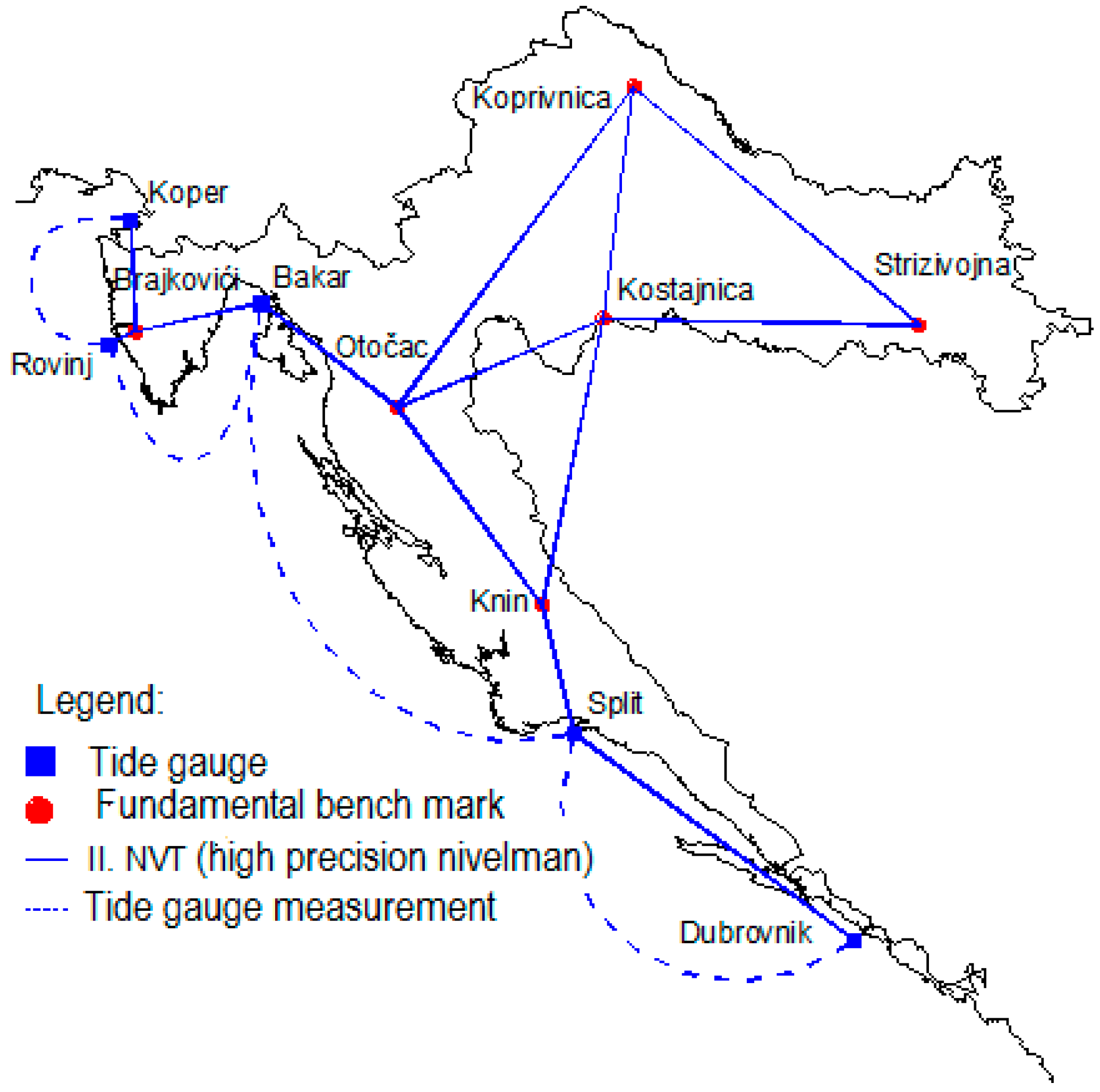
Tide gauge network establishment and data processing standards, including geodetic normal-null (N.N.), i.e., reference geoid surface level determination as reference vertical datums on the eastern Adriatic coast, are discussed.

(2)

It has been shown that the quality of TG data is satisfactory for the tide gauge network on the eastern Adriatic coast in the 20th century.

(3)

A redefinition of a new geodetic N.N. has recently been recommended to the relevant governmental authorities of Croatia instead of the used geodetic N.N. for the Adriatic Sea based on the sea level data in Trieste for 1875 only.

(4)

A comprehensive modelling of Earth’s crustal movements of the Adriatic micro-plate has also been presented.

(5)

A rising sea level trend was qualitatively detected in the broader Adriatic Sea area after interannual variations were removed (Figure 15).

(6)

On the bases of TG long-term sea level records, after removing crustal movement biases, spatially homogeneous sea level trends, on average about 2.43 mm/year, have been estimated for the eastern Adriatic coast for the period 1974–2018 (Table 4).

(7)

On the bases of satellite altimetry data for the whole Adriatic for the period 1993–2019, a positive sea level trend of about 2.6 mm/year was calculated as well (Section 2.4.3, second paragraph).

(8)

Application of Empirical Orthogonal Functions (EOFs) for reconstruction of sea level on a regular network (Section 3.1, second paragraph).

(9)

For the period 1880–2009, regional sea level rates from about −0.5 mm/year to 5 mm/year (Figure 18) and GMSL rates of about 1.5 mm/year (Section 3.2, second paragraph) were achieved and emphasized the complementarity and value of both satellite and tide gauge sea level data.

(10)

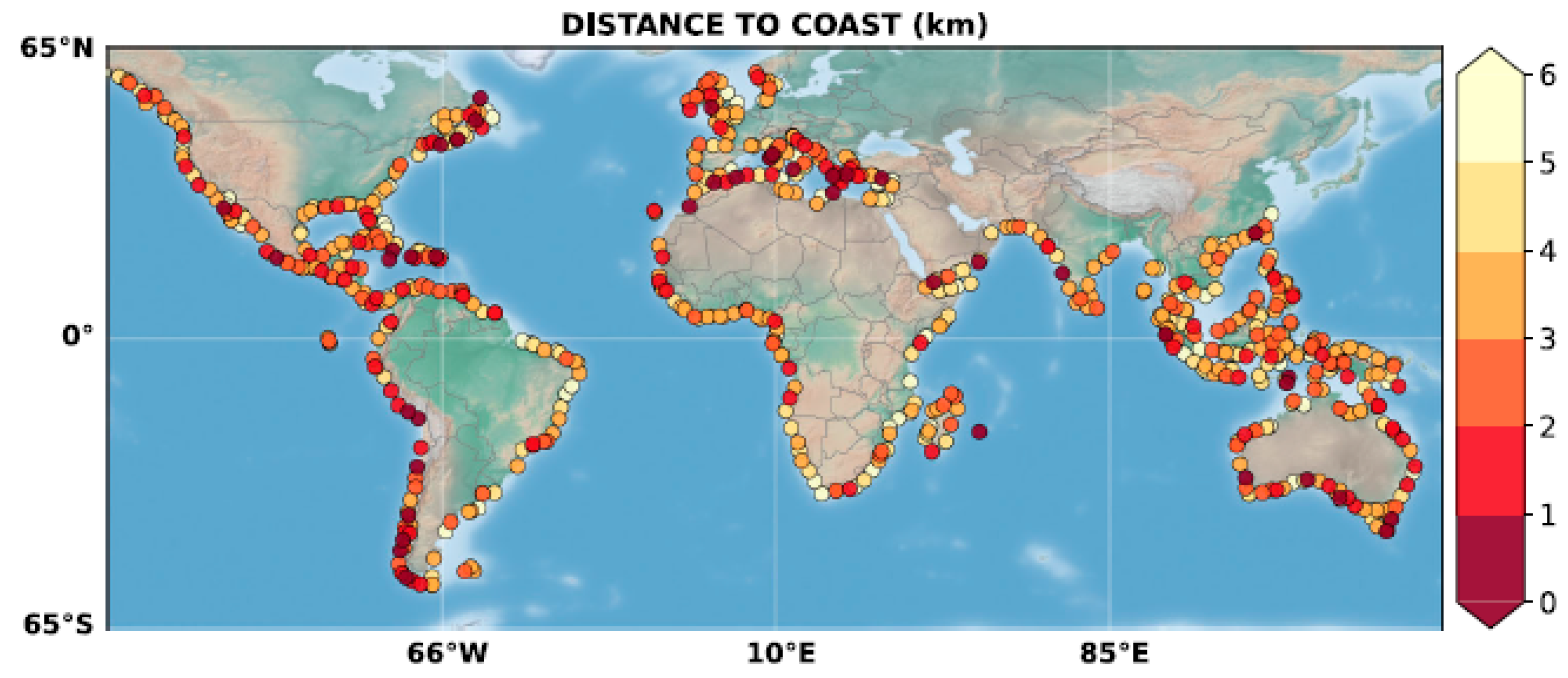
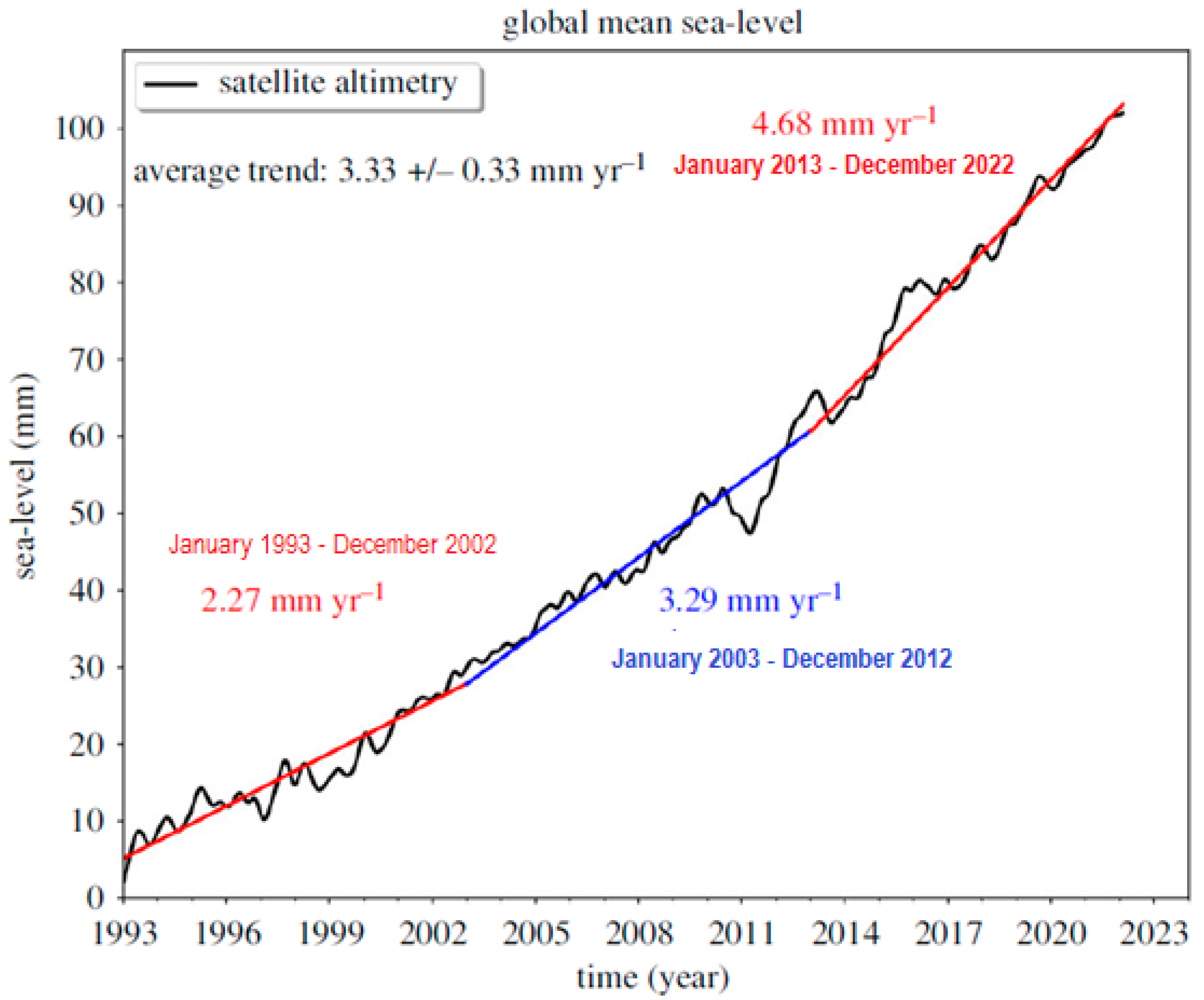
The possibility to compare the average mean sea level rise rate of 2.6 mm/year for the Adriatic Sea (Section 2.4.3, second paragraph) for the period 1993–2019 with the GMSL rise rate of 3.3 mm/year (Section 3.4, second paragraph) for the period 1993–2022 can be considered a big achievement.

(11)

Semi-empirical estimations of future sea level projections have been shown (Section 3.5). Unfortunately, the same sea level estimation procedure cannot be directly applied within semi-enclosed basins at mid-latitudes, such as the Adriatic and the Mediterranean Sea, at which the halosteric opposite effect was influential, at least in the period 1993–2019 (Section 2.4.3).

References

1. Church, J.A.; Woodworth, P.L.; Aarup, T.; Wilson, W.S. Understanding Sea Level Rise and Variability; John Wiley & Sons: Oxford, UK, 2010. [Google Scholar]
2. Orlić, M. An Introduction to Physical Oceanography; Element: Zagreb, Croatia, 2022. (In Croatian) [Google Scholar]
3. Seeber, G. Satellite Geodesy; Walter de Gruyter GMbH & Co.: Berlin, Germany, 2003. [Google Scholar]
4. Rožić, N. Croatian Height Reference System; Faculty of Geodesy University of Zagreb: Zagreb, Croatia, 2019; 256p. [Google Scholar]
5. Domijan, N.; Leder, N.; Čupić, S. Vertical datums of the Republic of Croatia. In Proceedings of the Third Croatian Congress on Cadastre, Croatian Geodetic Society, Zagreb, Croatia, 7–9 March 2005; Available online: https://www.hgd1952.hr/images/com_gallery_wd/uploads/3_KongresKatastar/3_KongresKatastar.pdf (accessed on 1 October 2023). (In Croatian).
6. Church, J.A.; White, N.J. A 20th century acceleration in global sea level rise. Geophys. Res. Lett. 2006, 33, 1–4. [Google Scholar] [CrossRef]
7. Guo, J.; Hwang, C.; Deng, X. Editorial: Application of Satellite Altimetry in Marine Geodesy and Geophysics. Front. Earth Sci. 2022, 10, 910562. [Google Scholar] [CrossRef]
8. Global Climate Observing System—GCOS. Implementation Plan for the Global Observing System in Support of the UnitedNations Framework Convention on Climte Change—UNFCCC (2010 Update). GCOS Rep.138. Available online: https://goosocean.org/index.php?option=com_oe&task=viewDocumentRecord&docID=6176 (accessed on 1 November 2023).
9. Bojinski, S.; Verstraete, M.; Peterson, T.C.; Richter, C.; Simons, A.; Zemp, M. The concept of essential climate variables in support of climate research, application and policy. Bull. Am. Meteorol. Soc. 2014, 95, 1431–1443. [Google Scholar] [CrossRef]
10. Kamranzad, F.; Memarian, H.; Zare, M. Earthquake Risk Assessment for Tehran, Iran. ISPRS Int. J. Geo-Inf. 2020, 9, 430. [Google Scholar] [CrossRef]
11. Laurenti, L.; Tinti, E.; Galasso, F.; Franco, L.; Marone, C. Deep learning for laboratory earthquake prediction and autoregressive forecasting of fault zone stress. Earth Planet Sci. Lett. 2020, 598, 117825. [Google Scholar] [CrossRef]
12. Lazos, I.; Sboras, S.; Chousianitis, K.; Bitharis, S.; Mouzakiotis, E.; Karastathis, V.; Pikridas, C.; Fotiou, A.; Galanakis, D. Crustal deformation analysis of Thessaly (central Greece) before the March 2021 earth quake sequence near Elassona-Tyrnavos (northern Thessaly). Acta Geodyn. Geomater. 2021, 18, 379–385. [Google Scholar] [CrossRef]
13. Santos-reyes, J.; Gouzeva, T.; Santos-reyes, G. Earth quake Risk Perception and Mexico City’s Public Safety. Procedia Eng. 2014, 84, 662–671. [Google Scholar] [CrossRef]
14. Kasumović, M. The Mean Level of the Adriatic Sea and the Geodetic Normal Null of Trieste. Rad Geofizičkog zavoda u Zagrebu 1950, 2, 1–22. Available online: https://hrcak.srce.hr/file/432951 (accessed on 1 November 2023).
15. Kasumović, M. On mean sea level of Adriatic Sea and its determination. Geod. List 1959, 13, 159–169. Available online: https://hrcak.srce.hr/file/432171 (accessed on 1 November 2023). (In Croatian).
16. Jovanović, B. Method Studies of: Sea Depth Observations and Its Data Processing and Definition of Coastal Line from Hidrographic, Geodetic and Marine Aspect. Ph.D. Thesis, Geodetic Faculty of University of Zagreb, Zagreb, Croatia, 1978; 292p. (In Croatian). [Google Scholar]
17. Bilajbegović, A.; Marchesini, C. Yugoslav vertical datums and preliminary relationship new Yugoslav nivelman with Austrian and Italian networks. Geod. List 1991, 45, 233–248. Available online: https://hrcak.srce.hr/293670 (accessed on 1 December 2023). (In Croatian).
18. Bašić, T. Unique transformation model and new geoid model of the Republic of Croatia. In Report on the Scientific Projects of State Geodetic Administration in Period from 2006 till 2009; Boseiljevac, M., Ed.; State Geodetic Administration: Zagreb, Croatia, 2009; pp. 5–21. Available online: https://www.researchgate.net/publication/228791071 (accessed on 1 October 2023). (In Croatian)
19. Dragičević, D.; Pavasović, M.; Bašić, T. Accuracy validation of official Croatian geoid solutions over the area of City of Zagreb. Geofizika 2016, 33, 183–206. [Google Scholar] [CrossRef]
20. Esselborn, S.; Rudenko, S.; Schöne, T. Orbit-related sea level errors for TOPEX altimetry at seasonal to decadal time scales. Ocean Sci. 2018, 14, 205–223. [Google Scholar] [CrossRef]
21. Marjanović, M.; Bačić, Ž.; Bašić, T. Determination of horizontal and vertical movements of the Adriatic micro-plate on the basis of GPS measurements. In Geodesy for Planet Earth, Proceedings of the 2009 IAG Symposium, Buenos Aires, Argentina, 31 August–4 September 2009; Springer: Berlin, Germany, 2012; Volume 136, pp. 683–688. Available online: https://link.springer.com/chapter/10.1007/978-3-642-20338-1_84 (accessed on 1 October 2023).
22. Omstedt, A.; Pettersen, C.; Rodhe, J.; Winsor, P. Baltic Sea climate: 200 yr of data on air temperature, sea level variations, icecover and atmospheric circulation. Clim. Res. 2004, 25, 205–216. [Google Scholar] [CrossRef]
23. Hammarklint, T. Swedish Sea Level Series—A Climate Indicator; Swedish Meteorological and Hydrological Institute: Stockholm, Sweden, 2009; Available online: https://www.smhi.se/polopoly_fs/1.8963!/Swedish_Sea_Level_Series_-_A_Climate_Indicator.pdf (accessed on 1 October 2023).
24. He, X.; Montillet, J.P.; Fernandes, R.; Melbourne, T.I.; Jiang, W.; Huang, Z. Sea level rise estimation on the pacific coast fromsouthern California to Vancouver island. Remote Sens. 2020, 14, 4339. [Google Scholar] [CrossRef]
25. Emery, K.O.; Aubrey, D.G. Sea Levels, Land Levels and Tide Gauges; Springer: New York, NY, USA, 1991; 245p. [Google Scholar]
26. Kapsi, I.; Kall, T.; Liibusk, A. Sea Level Rise and Future Projections in the Baltic Sea. J. Mar. Sci. Eng. 2023, 11, 1514. [Google Scholar] [CrossRef]
27. Cazenave, A.; Dominh, K.; Ponchaut, F.; Soudarin, L.; Cretaux, J.F.; Le Provost, C. Sea level changes from Topex-Poseidon altimetry and tide gauges and vertical crustal motions from DORIS. Geophys. Res. Lett. 1999, 26, 2077–2080. [Google Scholar] [CrossRef]
28. Kuo, C.Y.; Shum, C.K.; Braun, A.; Mitrovica, J.X. Vertical crustal motion determined by satellite altimetry and tide gauge data in Fenoscandia. Geophys. Res. Lett. 2004, 31, L01608. [Google Scholar] [CrossRef]
29. Wõppelmann, G.; Marcos, M. Coastal sea level rise in southern Europe and the no climate contribution of vertical land motion. J. Geophys. Res. 2012, 11, C01007. [Google Scholar] [CrossRef]
30. De Biasio, F.; Baldin, G.; Vignudelli, S. Revisiting vesrtical land motion and sea level trends in the north-eastern Adriatic Sea using satellite altimetry and tide gauge data. J. Mar. Sci. 2020, 8, 949. [Google Scholar] [CrossRef]
31. Surić, M. Reconstructing sea-level changes on the Eastern Adriatic Sea (Croatia)—An overview. Geoadria 2009, 14, 181–199. Available online: https://hrcak.srce.hr/clanak/68320 (accessed on 1 October 2023). [CrossRef]
32. Orlić, M. (Ed.) Nulla Dies Sine Observation—150 Years of Geophysical Institute in Zagreb; Geophysical Institute: Zagreb, Croatia, 2011. (In Croatian) [Google Scholar]
33. Orlić, M.; Pasarić, M. Sea level of Adriatic Sea and global climate changes. Pomor. Zb. 1994, 32, 481–501. Available online: https://www.croris.hr/crosbi/publikacija/prilog-casopis/182959 (accessed on 1 October 2023). (In Croatian).
34. Orlić, M.; Pasarić, M. Sea level changes and crustal movements recorded along the east Adriatic coastal waters. Nuovo C. Della Soc. Ital. Di Fis. C-Geophys. Space Phys. 2000, 23, 351–364. Available online: https://core.ac.uk/download/pdf/294761906.pdf (accessed on 15 November 2023).
35. Orlić, M.; Pasarić, M. Is the Mediterranean Sea level rising again? In Rapport du 40e Congres de la CIESM; CIESM: Marseille, France, 2013; p. 205. [Google Scholar]
36. Vilibić, I.; Šepić, J.; Pasarić, M.; Orlić, M. The Adriatic Sea: A long-standing laboratory for sea level studies. Pure Appl. Geophys. 2017, 174, 3765–3811. Available online: https://link.springer.com/article/10.1007/s00024-017-1625-8 (accessed on 15 November 2023). [CrossRef]
37. Kaplan, A.; Kushnir, Y.; Cane, M.A.; Blumenthal, M.B. Reduced space optimal analysis for historical datasets: 136 years of Atlantic sea surface temperatures. J. Geophys. Res. 1997, 102, 27835–27860. Available online: https://scholar.google.co.th/citations?user=-fMSJMoAAAAJ&hl=ja (accessed on 15 November 2023).
38. Chambers, D.P.; Mehlhaff, C.A.; Urban, T.J.; Fujii, D. Low-frequency variations in global mean sea level. J. Geophys. Res. 2002, 107, 3026. [Google Scholar] [CrossRef]
39. Church, J.A.; White, N.J.; Coleman, R.; Lambeck, K.; Mitrovica, J.X. Estimates of the regional distribution of sea level rise over the1950–2000 period. J. Clim. 2004, 17, 2609–2625. [Google Scholar] [CrossRef]
40. Curch, J.A.; White, N.J. Sea level rise from the late 19th to early 21st century. Surv. Geophys. 2011, 32, 585–602. Available online: https://link.springer.com/article/10.1007/s10712-011-9119-1 (accessed on 15 November 2023). [CrossRef]
41. Preisendorfer, R.W. Principal Component Analysis in Meteorology and Oceanography; Elsevier: Amsterdam, The Netherlands, 1988; 425p. [Google Scholar]
42. Pandžić, K. Principal component analysis of precipitation in the Adriatic-Pannonian area of Yugoslavia. J. Climatol. 1988, 8, 357–370. [Google Scholar] [CrossRef]
43. Pandžić, K.; Trninić, D. The relationship between the Sava River Basin annual precipitation, its discharge and thelarge-scale atmospheric circulation. Theor. Appl. Climatol. 1998, 61, 69–76. [Google Scholar] [CrossRef]
44. Pandžić, K.; Likso, T. Eastern Adriatic typical wind patterns and large-scale atmospheric conditions. Int. J. Clim. 2005, 25, 81–98. [Google Scholar] [CrossRef]
45. Chen, W.; Shum, C.K.; Forootan, E.; Feng, W.; Zhong, M.; Jia, Y.; Li, W.; Guo, J.; Wang, C.; Li, Q.; et al. Understanding water level changes in the Great Lakes by an ICA-based merging of multi-mission altimetry measurements. Remote Sens. 2022, 14, 5194. [Google Scholar] [CrossRef]
46. Dangendorf, S.; Hay, C.; Calafat, F.; Marcos, M.; Piecuch, C.G.; Berk, K.; Jensen, J. Persistent global sea level rise acceleration since the 1960th. Nat. Clim. Chang. 2019, 9, 705–710. Available online: https://www.nature.com/articles/s41558-019-0531-8 (accessed on 20 November 2023). [CrossRef]
47. Nerem, R.S.; Beckley, B.D.; Fasullo, J.T.; Hamlington, B.D.; Masters, D.; Mitchum, G.T. Climate change driven accelerated sea level rise detected in the altimeter era. Proc. Nat. Acad. Sci. USA 2018, 115, 2022–2025. [Google Scholar] [CrossRef] [PubMed]
48. Watson, C.S.; White, N.J.; Church, J.A.; King, M.A.; Burgette, R.J.; Legresy, B. Unabated global meansea-level rise over the satellite altimeter era. Nat. Clim. Chang. 2015, 5, 565–568. Available online: https://www.nature.com/articles/nclimate2635 (accessed on 15 November 2023). [CrossRef]
49. Cazenave, A.; Gouzenes, Y.; Birol, F.; Leger, F.; Passaro, M.; Calafat, F.M.; Shaw, A.; Nino, F.; Legeais, J.F.; Oelsmann, J.; et al. Sea level along the world’s coastlines can be measured by a network of virtual altimetry stations. Commun. Earth Environ. 2022, 3, 177. Available online: https://www.nature.com/articles/s43247-022-00448-z (accessed on 15 November 2023). [CrossRef]
50. Hamlington, B.D.; Gardner, A.S.; Ivins, E.; Lenaerts, J.T.M.; Reager, J.T.; Trossman, D.S.; Zaron, E.D.; Adhikari, S.; Arendt, A.; Aschwanden, A.; et al. Understanding of contemporary regional sea-level change and the implications for the future. Rev. Geophys. 2020, 58, e2019RG000672. [Google Scholar] [CrossRef] [PubMed]
51. International Altimetry Team. Altimetry for the future: Building on 25 years of progress. Adv. Space Res. 2021, 68, 319–363. [Google Scholar] [CrossRef]
52. Cazenave, A.; Moreira, L. Contemporary sea level changes from global to local scales: Areview. Proc. R. Soc. A 2022, 13, 1893. [Google Scholar] [CrossRef]
53. Horwath, M.; Gutknecht, B.D.; Cazenave, A.; Palanisamy, H.K.; Marti, F.; Marzeion, B.; Paul, F.; LeBris, R.; Hogg, A.E.; Otosaka, I.; et al. Global sea level budget and ocean mass budget, with focus on advanced data products and uncertainty. Earth Syst. Sci. Data 2022, 14, 411–447. [Google Scholar] [CrossRef]
54. Church, J.A.; Gregory, J.M.; Huybrechts, P.; Kuhn, M.; Lambeck, K.; Nhuan, M.T.; Qin, D.; Woodworth, P.L. Changes in sealevel. In Climate Change 2001: The Scientific Basis. Contribution of Working Group 1 to the Third Assessment Report of the Intergovernmental Panel on Climate Change; Houghton, J.T., Ding, Y., Griggs, D.J., Noguer, M., vander Linden, P., Dai, X., Maskell, K., Johnson, C.I., Eds.; Cambridge University Press: Cambridge, UK, 2001. [Google Scholar]
55. Meehl, G.A.; Stocker, T.F.; Collins, W.D.; Friedlingstein, P.; Gaye, A.T.; Gregory, J.M.; Kitoh, A.; Knutti, R.; Murphy, J.M.; Noda, A.; et al. Global climate projections. In Climate Change 2007: The Physical Science Basis. Contribution of Working Group 1 to the Fourth Assessment Report of the Intergovernmental Panel on Climate Change; Qin, D., Solomon, S., Manning, M., Marquis, M., Averyt, K., Tignor, M.M.B., Miller, H.L.J., Chen, Z., Eds.; Cambridge University Press: Cambridge, UK, 2007. [Google Scholar]
56. Rahmstorf, S. A semi-empirical approach to projecting future sea level rise. Science 2007, 315, 368–370. Available online: https://www.science.org/doi/abs/10.1126/science.1135456 (accessed on 15 November 2023). [CrossRef]
57. Hologate, S.; Jevrejeva, S.; Woodworth, P.; Brewer, S. Comment on A Semi-Empirical Approach to Projecting Future Sea-Level Rise. Science 135. Available online: https://www.science.org/doi/10.1126/science.1140942 (accessed on 15 November 2023).
58. Orlić, M.; Pasarić, Z. Semi-empirical versus process-basedsea level projections for the twenty-first century. Nat. Clim. Chang. 2013, 3, 735–738. Available online: https://www.nature.com/articles/nclimate1877 (accessed on 15 November 2023). [CrossRef]
59. Orlić, M.; Pasarić, Z. Some pitfalls of the semi-empirical method used to project sea level. J. Clim. 2015, 28, 3779–3785. [Google Scholar] [CrossRef]
60. IPCC. 2021: Summary for Policymakers. In Climate Change 2021: The Physical Science Basis. Contribution of Working Group I to the Sixth Assessment Report of the Intergovernmental Panel on Climate Change; Masson-Delmotte, V.P., Zhai, A., Pirani, S.L., Connors, C., Pean, S., Berger, N., Caud, Y., Chen, L., Goldfarb, M.I., Gomis, M., et al., Eds.; Cambridge University Press: Cambridge, UK, 2021. [Google Scholar]
61. Yang, L.; Lin, L.; Fan, L.; Liu, N.; Huang, L.; Xu, Y.; Metikas, S.P.; Jia, Y.; Lin, M. Satellite altimetry: Achievements and futuretrends by a scientometrics analysis. Remote Sens. 2022, 14, 3332. [Google Scholar] [CrossRef]
62. Tsimplis, M.N.; Raaicich, F.; Fenoglio-Marc, L.; Shaw, A.G.P.; Marcos, M.; Somot, S.; Bergamasco, A. Recent developments in understanding sea level rise at the Adriatic coast. Phys. Chem. Earth 2012, 40–41, 59–71. Available online: http://eprints.soton.ac.uk/id/eprint/159725 (accessed on 15 November 2023). [CrossRef]
63. Barić, A.; Grbec, B.; Bogner, D. Potential implications of sea level rise for Croatia. J. Coast. Res. 2008, 24, 299–305. Available online: https://www.jstor.org/stable/30137836 (accessed on 10 October 2023). [CrossRef]
64. Škreb, S. Sea level. Priroda 1936, 26, 271–274. Available online: https://library.foi.hr/dbook/cas.php?B=1&item=S00001&godina=1936&broj=00009&page=271 (accessed on 10 November 2023). (In Croatian).
65. Virual Surveyor. Available online: https://support.virtual-surveyor.com/en/support/solutions/articles/1000261346 (accessed on 10 December 2023).
66. von Sterneck, R. Kontrolie des Nivellementsdurchdie Flutmessrangaben und die Schwankungen des Meeresspiegels der Adria. In Mitteilungendse K. u. K. Militaägeographischen Institutes in Wien, Bd. XXIV; Military Institute in Vienna: Vienna, Austria, 1904. [Google Scholar]
67. Zupan, A. Average sea level for Split in the period 1947–1957. Hidrogr. Godišnjak 1958, 1956–1957, 123–151. (In Croatian) [Google Scholar]
68. Izvještaj o mareografskim osmatranjima na Jugoslavenskoj obali Jadranaza 1955., 1956.i 1957. Hydrographic Institute of Yugoslav Navy, Split, Croatia. 1956., 1957.i 1958. Available online: https://www.hhi.hr/en (accessed on 31 December 2022).
69. Vilibić, I.; Orlić, M.; Čupić, S.; Domijan, N.; Leder, N.; Mihanović, H.; Pasarić, M.; Pasarić, Z.; Srdelić, M.; Strinić, G. A new approach to sea level observations in Croatia. Geofizika 2005, 22, 21–57. Available online: http://geofizika-journal.gfz.hr/vol_22/vilibic.pdf (accessed on 15 November 2023).
70. Omar, K.; Ses, S.; Mustafar, M.A. The Malaysian seas: Variation of sea level observed by tide gauges and satellite altimetry. In Proceedings of the SEAMERGES Final Symposium, Bangkok, Thailand, 28 November–1 December 2005; Available online: http://eprints.utm.my/3518/1/Seamerges-salt-edited.pdf (accessed on 15 October 2023).
71. Lumban-Gaol, J.; Vignudelli, S.; Nurjaya, I.W.; Natih, N.M.N.; Sinurat, M.E.; Arhatin, R.E.; Kusumaningrum, E.E. Evaluation of altimetry satellite data products and sea level trends in the Indonesian maritime continent. Earth Environ. Sci. 2021, 944, 012041. Available online: https://iopscience.iop.org/article/10.1088/1755-1315/944/1/012041/meta (accessed on 15 November 2023). [CrossRef]
72. Andersen, O.B.; Nielsen, K.; Knudsen, P.; Hughes, C.W.; Bingham, R.; Fenoglio-Marc, L.; Gravelle, M.; Kern, M.; Poloo, S.P. Improving the coastal mean dynamic topography by geodetic combination of tide gauge and satellite altimetry. Mar. Geod. 2018, 41, 517–545. [Google Scholar] [CrossRef]
73. Hamden, M.E.; Din, A.H.M.; Wijaya, D.D.; Yusoff, M.Y.M.; Pa’suya, M.F. Regional mean sea surface and mean dynamic topography models around Malesian Seas developed from 27 years of Along-track satellite altimetry data. Front. Earth Sci. 2021, 9, 665878. [Google Scholar] [CrossRef]
74. Filmer, M.S.; Hughes, C.W.; Woodworth, P.L.; Featherstone, W.E.; Bingham, R.J. Comparison between geodetic and oceanographic approaches to estimate mean dynamic topography for vertical datum unification: Evaluation at Australian tide gauges. J. Geod. 2018, 92, 1413–1437. Available online: https://link.springer.com/article/10.1007/s00190-018-1131-5 (accessed on 15 November 2023). [CrossRef]
75. Pavasović, M.; Đapo, A.; Marjanović, M.; Pribičević, B. Present tectonic dynamics of the geological structural setting of the Eastern Part the Adriatic Region obtained from geodetic and geological data. Appl. Sci. 2021, 11, 5735. [Google Scholar] [CrossRef]
76. Dach, R.; Hugentobler, U.; Fridez, P. Bernese GPS Software Version 5.0 Tutorial; Astronomical Institute University of Bern: Bern, Switzerland, 2007; Available online: http://ftp.aiub.unibe.ch/BERN50/DOCU/DOCU50.pdf (accessed on 15 November 2023).
77. Altmer, Y.; Bačić, Ž.; Coticchia, A.; Medved, M.; Mulić, M.; Nurce, B. Present-day tectonics in and around the Adriaplate inferred from GPS measurements. In Postcollisional Tectonics and Magmatism in the Mediterranean Region and Asia; Dilek, Y., Pavlides, S., Eds.; Geological Society of America Special Paper 409; Geological Society of America: Bolder, CO, USA, 2006; pp. 43–55. [Google Scholar] [CrossRef]
78. Tsimplis, M.; Spada, G.; Marcos, M.; Flemming, N. Multi-decadal sea level trends and land movements in the Mediterranean Sea with estimation of factors perturbing tide gauge data and cumulative uncertainties. Glob. Planet Chang. 2011, 76, 63–76. [Google Scholar] [CrossRef]
79. Biondić, B.; Biondić, R. Hydrology of Dinaric Karst in Croatia; University of Zagreb: Zagreb, Croatia, 2014; 341p. (In Croatian) [Google Scholar]
80. Pandžić, K.; Cesarec, K.; Grgić, B. An analysis of the relationship between precipitation and discharge fields over a karstic river basin. Int. J. Climatol. 1997, 17, 891–901. [Google Scholar] [CrossRef]
81. Tsimplis, M.N.; Baker, T.F. Sea level drop in the MediterraneanSea. An indicator of deep water salinity and temperaturechanges? Geophys. Res. Lett. 2000, 27, 1731–1734. [Google Scholar] [CrossRef]
82. Tsimplis, M.N.; Josey, S.A. Forsing of Mediterranean Sea by atmospheric oscillations over the North Atlantic. Geophys. Res. Lett. 2001, 28, 803–806. [Google Scholar] [CrossRef]
83. Houghton, J.T.; Meira, L.G.; Callander, B.A.; Harris, N.; Kattenberg, A.; Maskell, K. (Eds.) Climate Change 1995: The Science of Climate Change; Cambridge University Press: Cambridge, UK, 1996; 572p. [Google Scholar]
84. Corti, S.; Molteni, F.; Palmer, T.N. Signature of recent climate change in frequencies of natural atmospheric circulation regimes. Nature 1999, 398, 799–802. Available online: https://www.nature.com/articles/19745 (accessed on 10 October 2023).
85. Meli, M.; Camargo, C.M.L.; Olivieri, M.; Slangen, A.B.A.; Romangoli, C. Sea level trend variability in the Mediterranean during the1993–2019 period. Front. Mar. Sci. 2023, 10, 1150488. [Google Scholar] [CrossRef]
86. Orlić, M. Basic physical properties and processes in theAdriatic Sea. In Velika geogrfija Hrvatske, Knjiga 2, Fizička geografija Hrvatske, Prirodno-geografska osnova razvoja; Školska knjiga; Sveučilište u Zadru, Odjel za geografiju, Školska knjiga: Zagreb, Croatia, 2023; pp. 485–513. (In Croatian) [Google Scholar]
87. Orlić, M.; Pasarić, M.; Pasarić, Z. Mediterranean sea level variability in the second half of the twentieth century: A Bayesian approach to closing the budget. Pure Appl. Geophys. 2018, 175, 3973–3988. [Google Scholar] [CrossRef]
88. Chen, X.; Zhang, X.; Church, J.A.; Watson, C.S.; King, M.A.; Monselesan, D.; Legresy, B.; Harig, C. The increasing rate of global mean se level rise during 1993–2014. Nat. Clim. Chang. 2017, 7, 492–495. Available online: https://polarice.geo.arizona.edu/papers/Chen.etal.AcceleratingGMSL.NClimate.2017.pdf (accessed on 15 November 2023). [CrossRef]
89. Budyko, M.I. On present-day climatic changes. Tellus 1977, 29, 193–204. [Google Scholar] [CrossRef]
90. Pandžić, K.; Likso, T.; Bonacci, O. A review of Extreme Air Temperature Analysis in Croatia. Atmosphere 2022, 13, 1893. [Google Scholar] [CrossRef]
91. Wang, Y.; Heidarzadeh, M.; Satake, K.; Mulia, I.; Yamada, M. A tsunami warning system based on off shore bottom pressure gauges and data assimilation for Crete Island in the Eastern Mediterranean Basin. J. Geophys. Res. Solid Earth 2020, 125, e2020JB020293. [Google Scholar] [CrossRef]
92. Frederikse, T.; Landerer, F.; Caron, L.; Adhikari, S.; Parkes, D.; Humphrey, V.W.; Dangendorf, S.; Hogarth, P.; Zanna, L.; Cheng, L.; et al. The causes of sea level rise since 1900. Nature 2020, 584, 393–397. Available online: https://www.nature.com/articles/s41586-020-2591-3 (accessed on 15 November 2023). [CrossRef] [PubMed]
93. Noye, B.J. Tide-well systems II: The frequency response of a linear tide-well system. J. Mar. Res. 1974, 32, 155–181. Available online: https://elischolar.library.yale.edu/cgi/viewcontent.cgi?article=2283&context=journal_of_marine_research (accessed on 15 October 2023).
Figure 1. The number and distribution of tide gauge stations: (A) temporal distribution of the number of stations with sea level data in the northern hemisphere (NH) and southern hemisphere (SH), respectively, and (B) spatial distribution of tide gauge staions in the 1980s (Adapted with permission from [6]).
Geohazards 05 00006 g001
Figure 2. Temporal coverage of the satellite altimetry missions which include sea level observations. Gray column, for the period between July 2022 and December 2004, overlaps with the period after reference [7] was published, and obviously, it is just part of missions’ projections until the end of 2024 (Adapted with permission from [7]).
Geohazards 05 00006 g002
Figure 3. The co-locations of TG and height benchmark (squares) on the northern and eastern Adriatic coast considered in the present review (Porto Corsini, Venice, Trieste, Rovinj, Bakar, Split—Marjan, Split—Port, Ston Mali, Broce, Dubrovnik, Herceg Novi and Bar) including the geodetic precise leveling train along the eastern Adriatic coast on the following route: Brajkovići (height benchmark only, red dot)—Pula—Rijeka—Lovinac (height benchmark only, red dot)—Split—Dubrovnik—Ulcinj (Adapted with permission from Ref. [63]).
Geohazards 05 00006 g003
Figure 4. The tide gauge in Bakar (after the Geophysical Institute of University of Zagreb, Croatia).
Geohazards 05 00006 g004
Figure 5. Relation of the Adriatic mean sea levels (MSLs) along of the Eastern Adriatic coast for Koper (KP), Rovinj (RO), Bakar (BA), Split (ST), Dubrovnik (DU), and Bar (BR) for the period 1954–1977 and N.N. for Trieste for the year 1875 (Adapted with permission from [16]).
Geohazards 05 00006 g005
Figure 6. Reference tide gauges on the eastern Adriatic Sea coast (Adapted with permission from Ref. [4]).
Geohazards 05 00006 g006
Figure 7. A highly reliable HRG2009 geoid solution for Croatia (Adapted with permission from Refs. [18,19]).
Geohazards 05 00006 g007
Figure 8. The basic concept of the satellite altimetry(Adapted with permission from Ref. [70]).
Geohazards 05 00006 g008
Figure 9. The average monthly and annual anomalies (mm), respectively, referred to as the multiannual averages for the period 1993–2012 for the coastal area of Croatia made by the satellite altimetry. Available at the World Bank web page: https://climateknowledgeportal.worldbank.org/country/croatia/impacts-sea-level-rise (accessed on 31 December 2022).
Geohazards 05 00006 g009
Figure 10. The mean sea levels (MSLs), in millimeters, for the tide gauge in Bakar for the period between 1930 and 2005. Missing data are indicated by blank (after [21]).
Geohazards 05 00006 g010
Figure 11. The ellipsoidal height data, in meters, for the Bakar GPS based on data of 21 GPS campaigns conducted in the period between 1994 and 2005 (after [21]).
Geohazards 05 00006 g011
Figure 12. The comparison of horizontal velocities of GPS stations. The black arrows indicate the solution from three GPS campaigns (1994–1998), the white arrows the solution from the last two GPS campaigns (1966–1998). The uncertainties of velocities are at the same level for both solutions. Due to the local effects, the magnitude and direction of velocity for the Bakar station (number 2) differ for both solutions; thus, local motion for this station has been assumed (after [77]).
Geohazards 05 00006 g012
Figure 13. (A) Slope angles and directions of annual velocities of geodetic points (for the period 2008–2013). Legend: 1—directions of annual velocity at geodetic points in mm/year; 2—spatially positive motions (uplift) greater than 0°, 20°, 30°, and 60°; 3—spatially negative motions (descending) greater than 0°, −30°; 4—maximum and minimum slope angles. (B) Slope angle and directions of annual velocities for Dubrovnik area (for more details, please see [75]).
Geohazards 05 00006 g013
Figure 14. Contemporary tide gauge records in southern Europe longer than 40 years with at least 80% valid data, including eastern Adriatic coast data. (Adapted with permission from Ref. [29]).
Geohazards 05 00006 g014
Figure 15. Time series of the tide gauge mean regional sea levels smoothed by a 5-year moving average (solid lines) for the Atlantic close to Gibraltar (1), the West Mediterranean (2), Adriatic Sea (3), and Black Sea (7). Cubic fits are superimposed to the time series (dashed lines). Please note that sea level trends for Ionian Sea (4), Levantine Basin (5), and Aegean Sea (6) are not considered here (after [35], adopted for this figure using authors’ presentations, and a personal communication).
Geohazards 05 00006 g015
Figure 16. Trend of total sea level (A), steric (B), thermosteric (C), and halosteric (D) components, calculated over satellite altimetry era (1993–2019). Black dots mark areas in which the trend is non-significant (95% CI). (Adapted with permission from Ref. [84]).
Geohazards 05 00006 g016
Figure 17. Global monthly and yearly averaged sea level between January 1950 and December 2000 from the reconstructed sea level fields. The results of TOPEX/Poseidon satellite are also shown (Adapted with permission from Ref. [39]).
Geohazards 05 00006 g017
Figure 18. The regional distribution of sea level rise rates between January 1950 and December 2000 from the reconstructed sea level data using EOF analysis. The solid line is 2.0 mm/year and contour interval is 0.5 mm/year (Adapted with permission from Ref. [39]).
Geohazards 05 00006 g018
Figure 19. Global average sea level from 1860 to 2009 reconstructed from the coastal and island sea level data (blue). The one standard deviation uncertainty estimates plotted about the low past sea level are indicated by shading. Values estimated in [6] for 1870–2001 are shown by the red solid line and dashed magenta lines for the 1 standard deviation errors. The series are set to have the same average values over 1960–1990 and the new reconstruction is set to zero 1990.The satellite altimetry data since 1993 are also shown in black (Adapted with permission from Ref. [40]).
Geohazards 05 00006 g019
Figure 20. GMSL from the HR and satellite altimetry during 1900–2015. (A) Time series of GMSL from the HR and AVISO satellite altimetry adjusted for the lower (GIA-based, 1.1 mm/year) drift correction from reference [48]. (B) Rates of GMSL rise as derived from an SSA with an embedding dimension of 10 years. (C) Acceleration coefficients as derived from 25-year moving quadratic fits. Also shown, as a black error bar, is the recent estimate from ref. [47] over the period 1993–2018. All shading represents the ± 1 s.e.m. (standard error of mean) point-wise uncertainties(Adapted with permission from Ref. [46]).
Geohazards 05 00006 g020
Figure 21. Global average of near-surface temperature for centered running 60-month periods, relative to the average for the 1991–2020 reference period (left-hand axis) and as an increase above the 1850–1900 level (right-hand axis), according to data of ERA% (C3S/ECMWF), JRA-55 (JMA), GISTEMPv4 (NASA), HadCRUT5 (Met Office Hadley Centre), NOAAGlobalTempv5 (NOAA), and Berkeley Earth. Credit: C35/ECMWF (Source: https://climate.copernicus.eu/climate-indicators/temperature (accessed on 31 December 2022)).
Geohazards 05 00006 g021
Figure 22. Distance to the coast of the 756 coastal virtual altimetry stations. Dots represent the locations of the virtual coastal stations and associated colors indicate the closest distance (km) to the coast reached by the first valid point along the Jason tracks (after [49]).
Geohazards 05 00006 g022
Figure 23. Global mean sea level time series (black curve) from multimission altimetry (data are from AVISO, https://www.aviso.altimetry.fr, accessed on 31 December 2022) from January 1993 to March 2022. The colored straight lines represent linear sea level trends over three successive time spans. (Adapted with permission from Ref. [52]).
Geohazards 05 00006 g023
Figure 24. Regional sea level trends from January 1993 to August 2022, based on multi-mission satellite altimetry. Data are from the Copernicus Climate Change Services, https://climate.copernicus.eu, (Online version in colour).
Geohazards 05 00006 g024
Figure 25. Global mean sea level budget during the period 1993–2016. The bottom curves refer to individual components. The black and red curves represent the altimetry-based GMSL time series and the sum of contributions, respectively. Shaded areas represent 1-sigma error (Adapted with permission from Refs. [52,53]).
Geohazards 05 00006 g025