Article

Convolutional Neural Network Classification of Exhaled Aerosol Images for Diagnosis of Obstructive Respiratory Diseases

1
Department of Biomedical Engineering, University of Massachusetts, Lowell, MA 01854, USA
2
Department of Electrical and Computer Engineering, University of California, Santa Cruz, CA 95064, USA
3
Department of Electrical and Computer Engineering, University of Illinois Urbana-Champaign, Urbana, IL 61801, USA
4
Department of Mechanical Engineering, California Baptist University, Riverside, CA 92504, USA
*
Author to whom correspondence should be addressed.
J. Nanotheranostics 2023, 4(3), 228-247; https://doi.org/10.3390/jnt4030011
Submission received: 17 April 2023 / Revised: 21 June 2023 / Accepted: 23 June 2023 / Published: 26 June 2023
(This article belongs to the Special Issue Emerging Strategies in Nanomedicine)

Abstract

:
Aerosols exhaled from the lungs have distinctive patterns that can be linked to the abnormalities of the lungs. Yet, due to their intricate nature, it is highly challenging to analyze and distinguish these aerosol patterns. Small airway diseases pose an even greater challenge, as the disturbance signals tend to be weak. The objective of this study was to evaluate the performance of four convolutional neural network (CNN) models (AlexNet, ResNet-50, MobileNet, and EfficientNet) in detecting and staging airway abnormalities in small airways using exhaled aerosol images. Specifically, the model’s capacity to classify images inside and outside the original design space was assessed. In doing so, multi-level testing on images with decreasing similarities was conducted for each model. A total of 2745 images were generated using physiology-based simulations from normal and obstructed lungs of varying stages. Multiple-round training on datasets with increasing images (and new features) was also conducted to evaluate the benefits of continuous learning. Results show reasonably high classification accuracy on inbox images for models but significantly lower accuracy on outbox images (i.e., outside design space). ResNet-50 was the most robust among the four models for both diagnostic (2-class: normal vs. disease) and staging (3-class) purposes, as well as on both inbox and outbox test datasets. Variation in flow rate was observed to play a more important role in classification decisions than particle size and throat variation. Continuous learning/training with appropriate images could substantially enhance classification accuracy, even with a small number (~100) of new images. This study shows that CNN transfer-learning models could detect small airway remodeling (<1 mm) amidst a variety of variants and that ResNet-50 can be a promising model for the future development of obstructive lung diagnostic systems.

Graphical Abstract

1. Introduction

Despite their chaotic appearances, exhaled aerosols and their patterns contain information that is inherent to the underlying respiratory physiology and anatomy [1,2,3,4,5]. For a given person, a different exhaled aerosol pattern may be associated with a change in the respiratory airway geometry or function [6,7,8]. Following this hypothesis, exhaled aerosols can be explored for their potential to detect the disease’s presence, estimate the disease severity level, and localize the disease site [9,10,11,12]. However, characterizing and distinguishing subtle differences in aerosol patterns can be highly challenging. For small airway diseases, where disturbance signals are weak, the challenge is even greater. These signals can be further weakened by exhaled air from the disease site to the mouth opening. Hence, it is essential to determine if these weak signals can be detected at the mouth and utilized to detect airway diseases at early stages [13,14,15,16,17].
Machine learning algorithms have been tested to develop intelligent diagnostic systems for obstructive lung diseases using exhaled aerosols [18]. The major challenge when using a machine learning algorithm such as SVM or random forest is that predefined features are needed for training [19]. Moreover, the prediction sensitivity and specificity are mostly dependent on the quality of the extracted features from the source dataset. The exhaled aerosol images are particles deposited on a filter in the mouthpiece. The particle distributions often exhibit a highly complex pattern and are difficult to characterize. Moreover, the differences in the exhaled aerosol patterns between health and disease can be subtle and cannot be readily distinguished with human eyes. Predefined features, such as fractal dimension and dynamic mode decomposition (DMD), only captured partial information about the images [20,21]. The question of whether these predefined features are most relevant to airway remodeling (structural variation) is unclear. Moreover, the inherent differences may be multifaceted, which makes it a more appropriate problem to use deep convolutional neural networks, where convolutional layers of different layers may capture or retain different disease-associated features at different scales.
Convolutional neural networks (CNNs) have gained popularity in recent years due to their superior performance in image classification compared to traditional machine learning algorithms. One attractive aspect of CNNs is their ability to perform feature extraction and classification simultaneously. They can learn rich features at multiple levels, resulting in successful applications in medical image analysis. However, applying CNN models to medical images presents unique challenges. Effective model training typically requires large datasets, but high-quality medical images are often scarce. In one study [19], we tested a database of 405 images and found it sufficient for SVM and random forest classifications but inadequate for meaningful deep learning tests. As more medical image data becomes available, it is important to evaluate the performance of CNN models in analyzing exhaled aerosol images.
Transfer learning has become increasingly popular in medical image-based diagnostic systems based on existing CNN models such as AlexNet, GoogleNet, ResNet, DenseNet, MobileNet, etc. [22,23,24]. However, CNN-based transfer learning sometimes does not perform as expected, giving unexpectedly lower prediction accuracy in the testing stage despite a high accuracy rate in the training and validation stages [25]. For a given medical image dataset, which usually has a limited number of images and small image differences, overfitting is a common problem using the popular CNN models, which often have over 10 layers with 60+ million trained parameters and have been trained on a large dataset (imageJ) containing 1000 categories. By contrast, the features of medical images are limited; the differences between the images are subtle and are often not perceivable/discernible to our human eyes. These lower testing properties may be associated with the fact that the features/filters/convolutional layers trained on ImageJ may be distinct from those of the medial images [26]. The transfer learning predictions, which adapted the initially irrelevant filters to the new image dataset, could retain features that are not that relevant to the images and contaminate the scoring process for classification.
The objective of this study was to evaluate the performance of different pre-trained CNN models (i.e., AlexNet, ResNet-50, MobileNet, and EfficientNet) in detecting and staging small airway abnormalities from exhaled aerosol images. Specific aims include:
(1)
To assess model capacity in classifying images inside and outside the design space;
(2)
To quantify the benefits of continuous learning on the model’s performance;
(3)
To evaluate the relative importance of breath test variables on classification decisions;
(4)
To select an appropriate CNN model for the future development of obstructive lung diagnostic systems based on exhaled aerosol images.

2. Methods

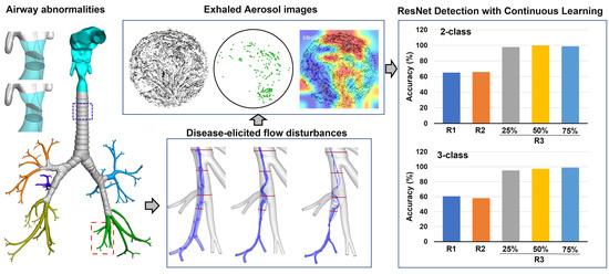
2.1. Normal and Diseased Airway Models

Physiology-based modeling and simulations were used to generate images of exhaled aerosols from normal and diseased airways under varying breathing conditions. The normal airway model was developed by Xi et al. [27,28], which extended from the mouth up to the ninth generation (G9) lung bifurcations and retained 125 bronchial outlets (Figure 1a). In this study, the airway obstruction occurred at G7-9 bronchioles, whose diameters were less than 1 mm (i.e., small airways). Therefore, the obstruction was also smaller than 1 mm in size, which was below the smallest nodule size to be detected using X-rays or CT scanning (3–4 mm) [29]. Note that the model-generated images could be less complex than real-life images and might be less challenging to differentiate. Thus, we hypothesized that by considering the airway lesions that were below the detection limit of current radiological imaging technologies, it was anticipated that the proposed computer-aided diagnostic system could achieve sufficiently high diagnostic accuracy when applied in clinical settings.
The morphology of the normal mouth-lung model (D0) was modified to generate two diseased models (D1, D2) in the left lower lobe (red dashed rectangle, Figure 1a). In doing so, Hypermorph (Troy, MI) was used to shrink the bronchioles at G7-9 twice (D1, D2, Figure 1a). Similarly, the normal throat opening, or glottal aperture, was progressively decreased by 1 mm, 2 mm, and 3 mm to generate three constricted throats (Th1, Th2, and Th3, Figure 1a). The normal and modified airway models were subsequently meshed using Ansys ICEMCFD for fluid-particle simulations (Figure 1b).

2.2. Numerical Methods for Image Generation

ANSYS ICEMCFD was applied to create the computational mesh in the mouth-lung airway geometries. To sufficiently resolve the drastic flow variation in the near wall region, body-fitted meshes were generated that contained a five-layer prism mesh. A grid-independent study was conducted by varying mesh densities from coarse to ultrafine. Grid-independent results were achieved at 4.8 million tetrahedral cells with five layers of prismatic cells and a near-wall cell height of 50 µm [27,30,31]. ANSYS Fluent (Canonsburg, PA, USA) was used to simulate the inhalation/exhalation flows and generate the exhaled aerosol images. During the inhalation, particles were injected into the mouth and exited from the lung. During the exhalation, the particles reversed their direction to enter the bronchioles and travel through the respiratory tract. Their positions were recorded at the mouth opening, and their distribution pattern collectively formed the exhaled aerosol image to be used in the subsequent CNN training and/or testing.
The turbulent k-ω model was used to simulate the inhalation and exhalation airflows. Ambient pressure was prescribed at the mouth opening. Negative/positive pressures were specified to generate a prescribed inhalation/exhalation flow rate. The particle motion was tracked with a Lagrangian discrete phase model (DPM). Particles are deposited on the airway wall upon contact. Considering the dilute nature of the particles, one-way coupling (i.e., flow to particles) was assumed during the particle tracking. User-defined MATLAB codes were developed to generate particles at the mouth inlet and reverse the particle velocities at the bronchiolar outlets. Different test cases were simulated with varying inhalation/exhalation flow rates, particle sizes, and airway geometries, as illustrated in Figure 2a–d. One exhalation aerosol image required one inhalation, one exhalation, and particle tracking, which required approximately 4 h, 4 h, and 10–90 min, depending on the particle size, respectively, in an AMD Ryzen 3960X 24-Core workstation with 3.79 GHz processors, 256 G RAM, and an 8 G GPU. For a total of 2745 images used in this study (11 flow rates, 4 geometrical models), a cumulative of 3200 computational hours or so were used.

2.3. Data Architecture

In the baseline dataset (Base), the throat was kept constant in the three airway models (D0, D1, and D2). The recommended range (or design space) of the breath tests included particle sizes ranging 0.5–10 µm and flow rates ranging 10–19 L/min. Specifically, the particle sizes considered included 0.5, 0.6, 0.7, 0.8, 0.9, 1, 2, 3, 5, 7, 9, and 10 µm, while the respiratory flow rates included 10, 12.5, 14.5, 15, 16.5, 17, 17.5, 18, 18.5, 18.5, and 19 L/min. In total, the baseline dataset contained 1080 images, of which 90% were used for training and 10% for testing in Round 1 (cycles of varying colors in Figure 2a,b).
The inbox database included 535 images with either particle size or flow rate that were never seen in the baseline database. However, these particle sizes and flow rates were still within the design space. Two separate folders were generated, with one having a flow rate of 13.5 L/min (Inbox_Q, green triangles in Figure 2a) and the other having particle sizes of 2.5, 4, 6, and 8 µm (Inbox_dp, pink asterisks in Figure 2a), which was also summarized in Figure 2c.
The outbox database included 649 images and represented scenarios outside of the design space. These included different flow rates (i.e., 20, 21, and 22 L/min, termed Outbox_Q: black diamonds and Outbox_Q_dp: blue asterisks in Figure 2a), geometries (varying glottal apertures, termed as Outbox_Th), and their combinations (Outbox_Q_dp and Outbox_Q_dp_Th), as shown in Figure 2d. It noted that the images with 2.5, 4, 6, and 8 µm (pink and blue asterisks) were reserved for testing only and have never been included in the training datasets.

2.4. Design of CNN Model Training/Testing

Four convolutional neural network (CNN) models were selected in this study: AlexNet, EfficientNet, MobilNet, and ResNet-50. AlexNet and ResNet were selected because they were the 2012 and 2014 winners of the ImageNet competition, respectively [32,33]. AlexNet was groundbreaking in its use of GPUs for training deep neural networks, while ResNet introduced residual connections between different layers to improve gradient flow and enable the training of even deeper neural networks [34,35]. EfficientNet and MobilNet were chosen for their simpler architecture and smaller computational requirements [36,37,38,39]. It will be desirable to run a computer-aided diagnostic (CAD) system on a personal computer or even a smartphone, provided it can achieve sufficient diagnostic accuracy. This study employed both Python and MATLAB platforms for CNN model training/testing, and the performance results were compared between the corresponding cases. For each model, all network layers were kept identical during training, and only the number of outputs in the classification layer was changed to match the classification task (two-class or three-class). Thus, an ablation study was not performed that selectively removed or modified certain components or hyperparameters to assess their individual contributions to the model’s performance.
The training/testing processes are shown in Table 1. There were three rounds of training and testing. In each round, testing was conducted on three datasets with varying levels of similarity to the training datasets. By training one model several rounds with augmented datasets and testing its performance for datasets with decreasing similarities, it was aimed to (1) select the optimal CNN model, (2) test the model’s ability to extrapolate, and (3) test the model’s ability to learn from new data.
In Round 1, we aimed to validate a model (i.e., level 1) as well as test whether the model could predict new samples within (level 2) and outside (level 3) the design space. In doing so, 90% of the baseline was used for training and 10% was set aside for validation purposes (level 1). The level 2 test database included two folders with either different flow rates (Inbox_Q) or particle sizes (Inbox_dp, Figure 2c). Similarly, the level 3 database also included two folders, with either outbox flow rates (i.e., 20, 21, 22 L/min, Outbox_Q) or modified throats (Outbox_Th), as shown in Figure 2d.
In Round 2, new images with varying levels of throat constriction (Outbox: Th1 and Th2) were added to the training dataset. The newly trained model would be tested at three levels. Because new features related to the throat variation were added, the classification results for the outbox dataset should be improved.
In Round 3, additional images with Outbox flow rates (20, 21, and 22 L/min) were introduced into the training dataset to enhance the model’s performance. To determine the minimum number of images required to attain a notable improvement, various proportions of the Outbox images (25%, 50%, and 75%) were included in the training dataset. The newly trained models subsequently underwent testing on the Level 1, Inbox, and Outbox test datasets to assess their performance.
For each training, a 10-fold cross-validation approach was adopted, where the baseline dataset was randomly divided into 10 subgroups. This approach ensured that each subgroup was used once for validation and the remaining nine subgroups for training. Given that every subgroup was used for both training and validation at some point, this approach facilitated a more robust and unbiased estimation of the models’ performance. To mitigate the class imbalance in the dataset, several data augmentation strategies were implemented, including random rotation (‘RandRotation’: [−5° 5°]), random reflections across both axes (‘RandXReflection’: 1, ‘RandYReflection’: 1), and random shearing in both the x and y dimensions (‘RandXShear’: [−0.05 0.05], ‘RandYShear: [−0.05 0.05]). By increasing the size and variety of the minority class, a more balanced class distribution could be obtained, which mitigated bias towards the majority class and thus improved the model’s performance. All models were trained on a workstation with an Intel 9900k processor, an RTX 2070 Super GPU, and 128 G RAM. With a 10-fold cross-validation, the training time was around 80 min for AlexNet, 100 min for ResNet-50, 70 min for EfficientNet, and only 5 min for MobileNet. This indicated that these transfer learning models could be trained in an efficient manner despite their inherent complexities. Note that MobileNet, known for its streamlined architecture, demonstrated much faster training times than the deeper ResNet-50 and AlexNet models. To evaluate the network classification performance, various indices were quantified, including the accuracy, sensitivity, specificity, precision, AUC (area under curve), and ROC (receiver operating characteristic) curve.

3. Results

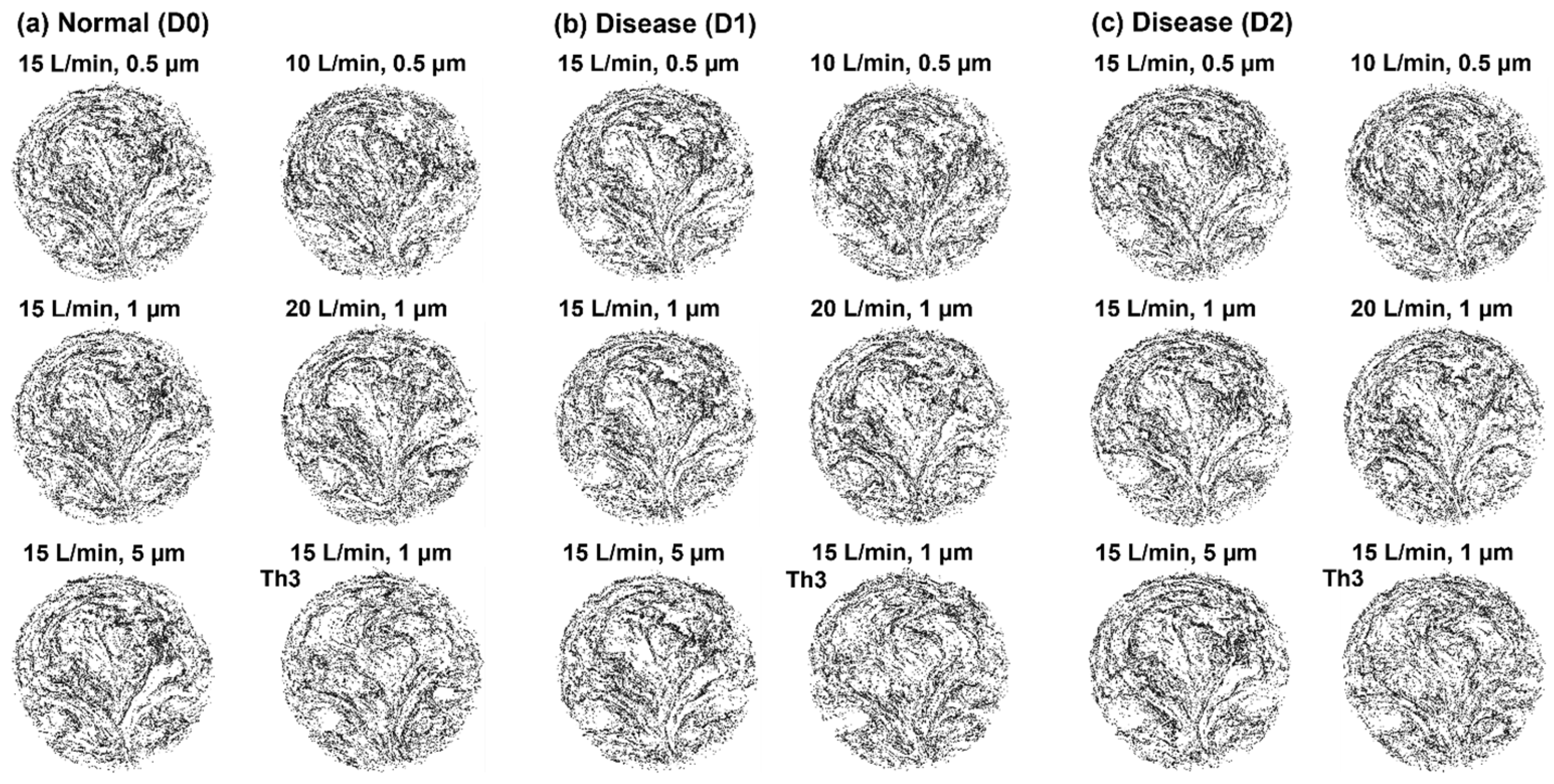
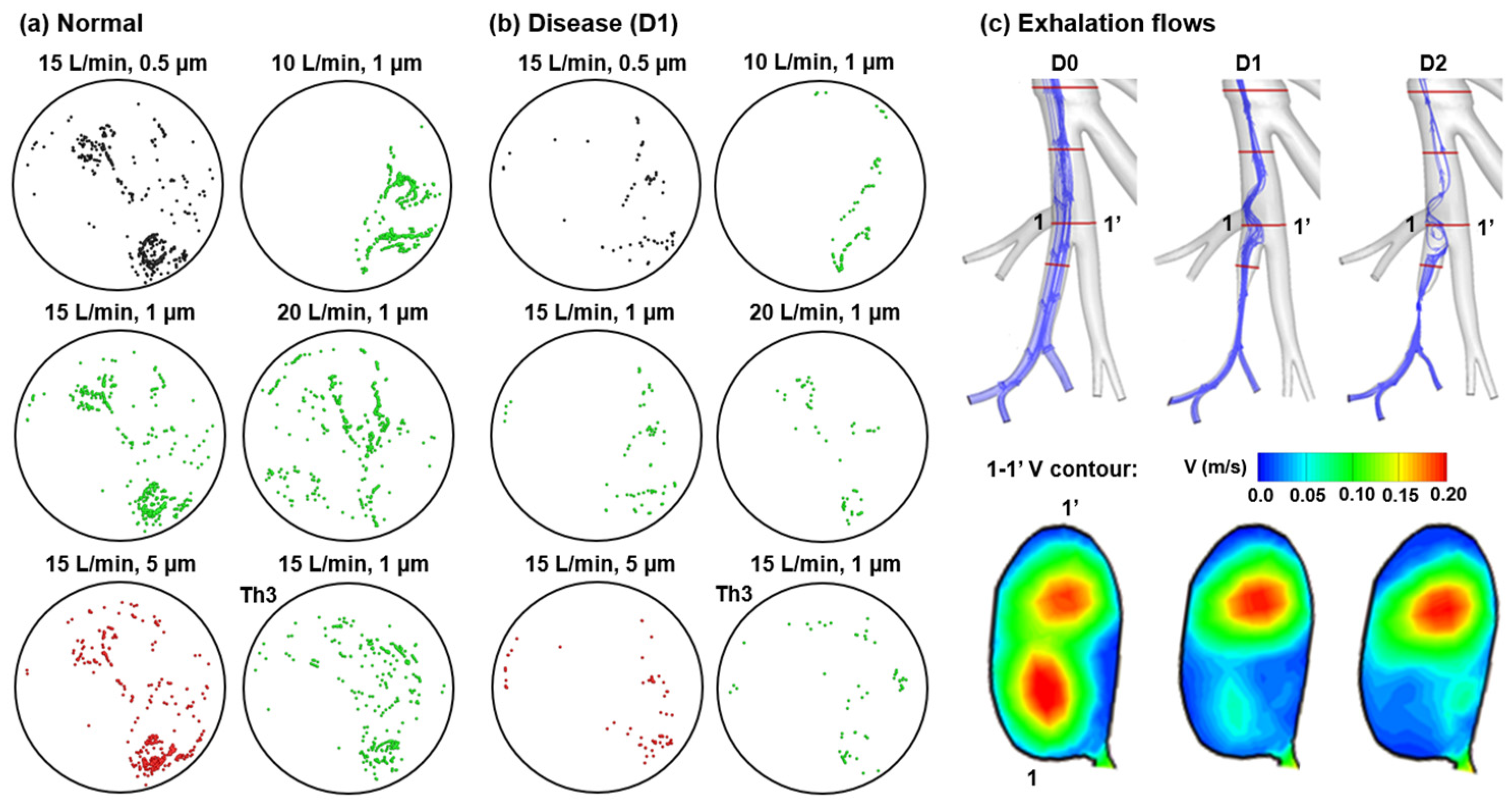
3.1. Exhaled Aerosol Images at Mouth Opening

3.1.1. Cumulative Aerosol Images

The exhaled aerosol images obtained from physiology-based simulations are shown in Figure 3a–c for the normal airway (D0), stage 1 disease (D1), and stage 2 disease (D2), respectively. Under each category, aerosol images are presented for different particle sizes (0.5, 1, and 5 µm), flow rates (10, 15, and 20 L/min), and throat opening (normal vs. Th3). One major characteristic of these images is their complex appearance, which may seem chaotic at first glance. A closer inspection reveals some regular patterns in these images, with fine, subtle discrepancies in these patterns among different images and between health (Figure 3a) and diseases (Figure 3b,c). These exhaled aerosol images can be considered a conference of many particle scouts that travel through the lung and come back to the mouth opening to report what they have experienced. Because the trajectory of a particle is dictated by the lung geometry it traveled through, any airway structural change will cause a disturbance to the particle motion and deposit it at a different position on the filter at the mouth opening. It is thus possible that all these scout particles collectively telltale the health of the lung. Considering that a severe airway remolding will affect more particles, the resultant particle patterns should differ more from normal and can be used to correlate to the disease severity.

3.1.2. Disease-Associated Aerosol Distributions

To understand the disease-associated flow disturbance and particle trajectories, particles were released only from the disease-afflicted bronchioles during exhalation. The resultant particle distributions at the mouth opening are shown in Figure 4a,b for the normal and mildly constricted (D1) lungs. Compared to the normal condition, much fewer particles were exhaled from the diseased bronchioles for two reasons: (1) fewer particles reached this region during inhalation due to reduced ventilation, and (2) the flow disturbance in this region made it more likely for exhaled particles to deposit. For the same reason, nearly no particles were exhaled from the severely constricted (D2) bronchioles (Figure not shown). Figure 4c compares the expiratory stream traces and velocity contours in the disease-affected bronchioles, which differ notably among the three models (D0, D1, and D2).
Further insights into the image-disease correlation can be obtained by examining the particle responses to disease-elicited disturbances under varying breathing conditions. First, for a given flow rate (15 L/min, first column), similar particle distributions were observed among particles of 0.5, 1, and 5 µm. This was interesting because theoretically, the particle response time (τp = ρdp2/18 µ) varied with dp2; the observed small discrepancies among particles at 15 L/min resulted from the fact that the τp for 0.5–5 µm particles was much smaller than the flow time. This also explained the much larger differences in particle distributions among different flow rates (10, 15, and 20 L/min) (Figure 4a,b).
One interesting observation was made regarding the distribution of 1-µm particles with throat variation of Th3. At a flow rate of 15 L/min, the distribution resembled the corresponding case of Th0, but it differed significantly from the distributions at 10 and 20 L/min. This observation prevailed for both normal and disease conditions (Figure 4a,b), suggesting that flow rate had a greater impact on particle distribution than particle size or throat variation.

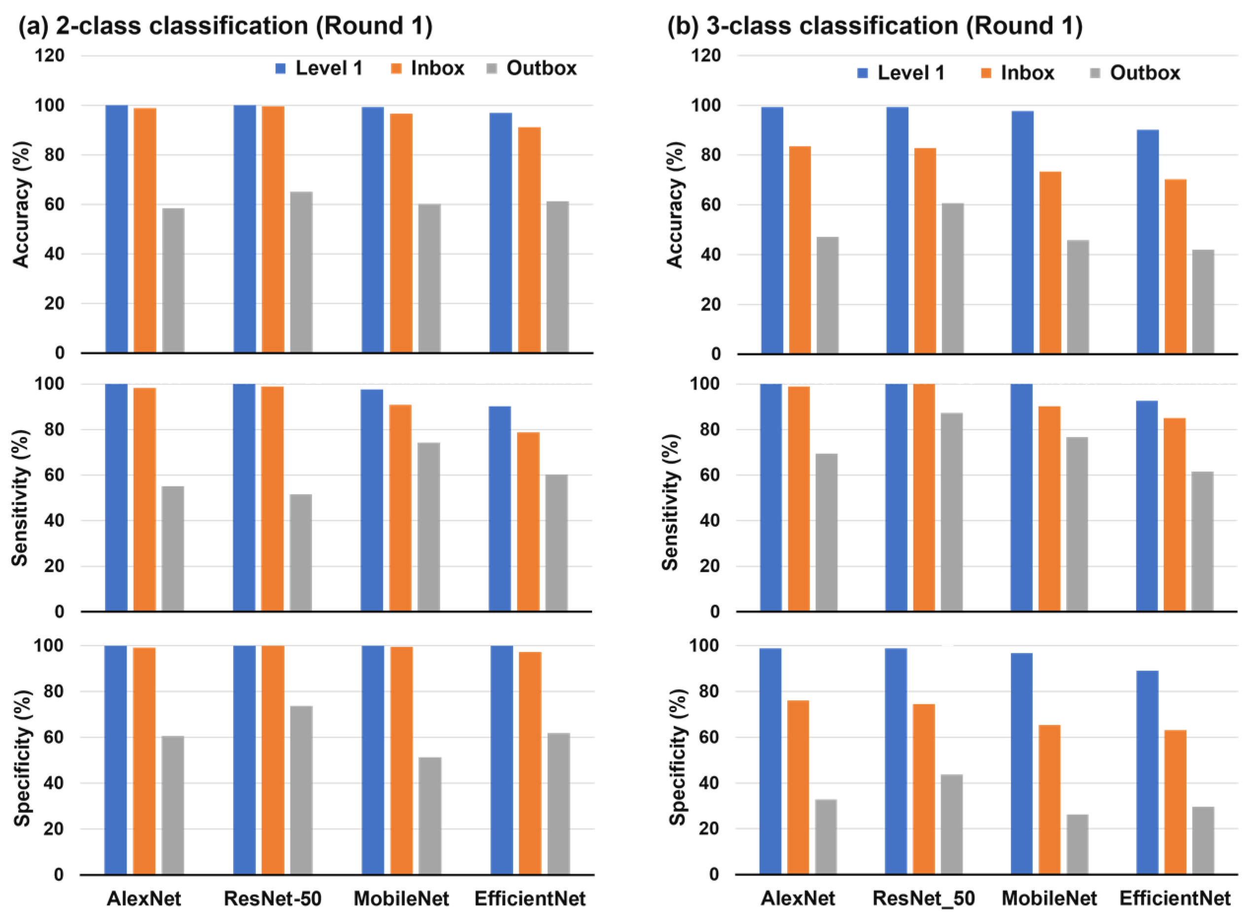
3.2. Round 1 Training/Testing

3.2.1. Test Data with Decreasing Similarities

In Round 1, the four models (AlexNet, EfficientNet, MobileNet, and ResNet-50) were trained on the 90%-base dataset, as defined in Figure 2, and represented the first-generation diagnostic system. Their performances tested on samples with decreasing similarities (Level 1, Inbox, and Outbox) are summarized in Table 2. In this study, Level 1 testing was equivalent to validation, while Inbox and Outbox testing signified the model’s ability for interpolation within and extrapolation out of the design space, respectively.
For the 2-class classification task (i.e., normal vs. disease, in Table 2 and Figure 5a), both AlexNet and ResNet-50 achieved 100% accuracy on the Level 1 dataset; MobileNet and EfficientNet also achieved high accuracy on Level 1, i.e., 99.24% and 96.97%, respectively. All models gave slightly lower classification accuracy on the Inbox dataset, which was expected considering that Inbox images still came from the same design space, although their exact operating conditions (flow rate and particle size) had not been considered by the model. These similarly high accuracies between the Level 1 and Inbox datasets indicated that all models herein had a satisfactory interpolation capacity for the 2-class classification. In other words, their response surface spanning the design space was not highly nonlinear. This observation was also valid for sensitivity and specificity (Figure 5a, middle and lower panels). By contrast, the performance dropped significantly on the Outbox set for all modes considered (Figure 5a), indicating a poor extrapolation capacity or an increasingly nonlinear response surface outside the design space.
For the three-class classification task (D0 vs. D1 vs. D2, in Table 2 and Figure 5b), significantly lower accuracies were obtained on both the Inbox and Outbox sets, even though the accuracy on Level 1 was still high. It was thus much more challenging to classify more than two categories (such as disease staging) than a 2-class disease detection. In particular, the specificity, which measures the network’s ability to correctly identify negative samples, significantly dropped (Figure 5b, lower panel).

3.2.2. Comparison of Model Performance

Network performances in 3-class clarification were further compared in Figure 6a. Among the four models, EfficientNet had the lowest overall performance across all three test data sets in both accuracy and sensitivity (Figure 6a). Even though not necessarily the direct cause, EfficientNet used the sigmoid-based Swish activation function as opposed to the ReLU function in the other three models [40,41,42]. Regarding the Inbox set, AlexNet and ResNet-50 maintained higher performance than the two simpler models. Regarding the Outbox set, ResNet-50 excelled over the other three models in all indices considered, with a margin of 15.7 ± 2.6% in accuracy, 18.1 ± 7.5 in sensitivity, and 14.1 ± 3.3 in specificity (Figure 6a and Table 2). By contrast, AlexNet’s performance dropped more significantly on the Outbox set; both the ROC profile (Figure 6b) and AUC (Table 2) were the lowest among models, reflecting AlexNet’s poor performance outside of the design space.

3.3. Continous Training/Testing
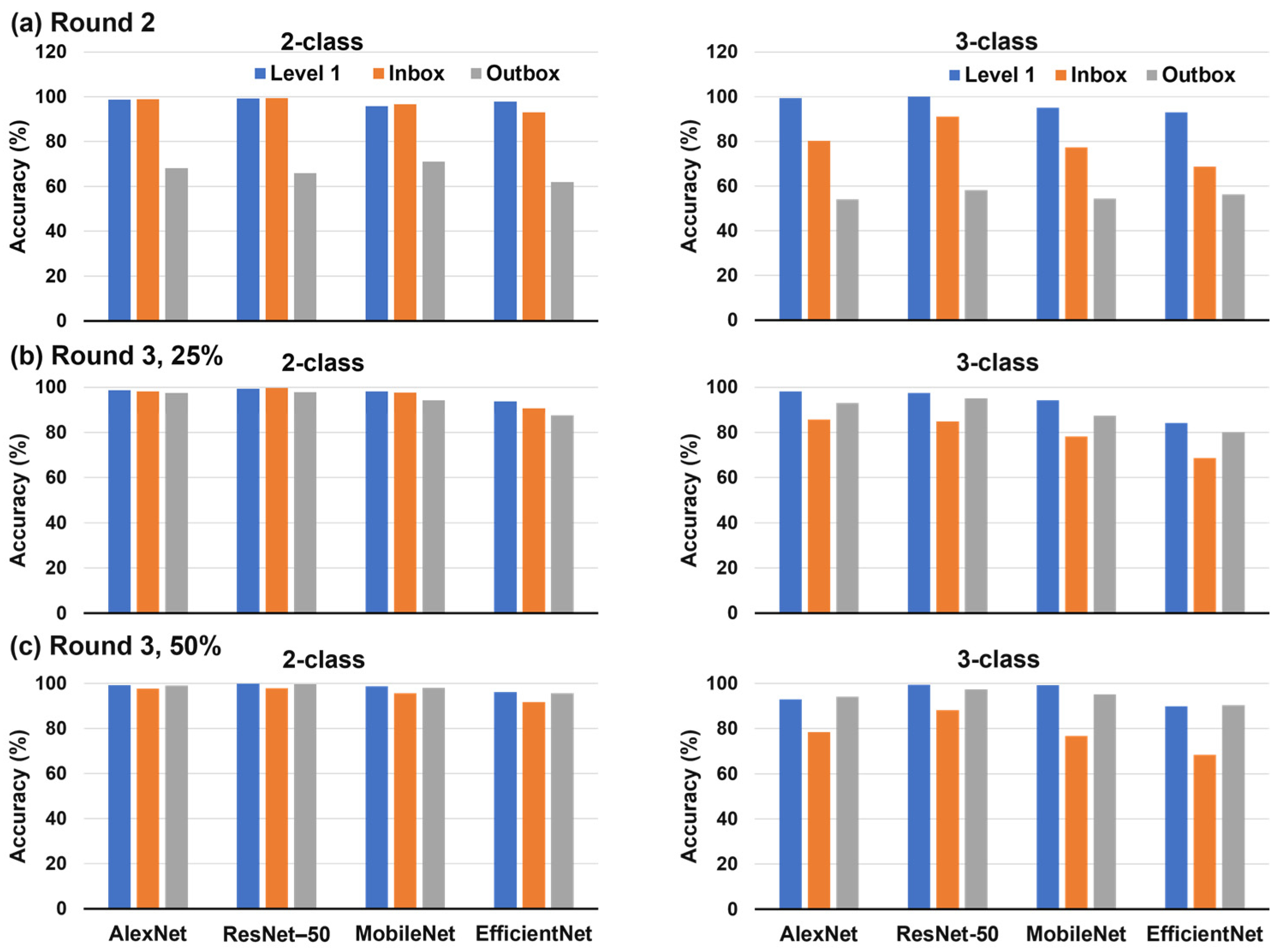
3.3.1. Round 2

The reduced performance on the Outbox data set could result from three factors: a different throat opening, flow rate, or particle size. Considering that the network training in Round 1 did not include information on varying throat openings, new images from Th1 and Th2 were added to the Round-1 training set (90% Base), as shown in Table 1. All network models were trained again on the new data and tested on Level 1, Inbox, and Outbox sets (Figure 7a and Table 3). As expected, for the 2-category classification, all models maintained high accuracies on the Level 1 and Inbox data sets. Improved performances on the Outbox images were observed in AlexNet and MobileNet; however, only limited improvement was observed in ResNet-50 and EfficientNet (Figure 7a, left panel). Similar observations were also made for the more challenging 3-class classification task (Figure 7a, right panel). This might be attributed to influencing factors other than the throat opening variation, such as the flow rate (20–22 L/min) outside the design space (10–19 L/min), which had not been included in the Round 2 training.

3.3.2. Round 3, 25% Outbox

Further training was conducted by adding 25% of Outbox images to the training dataset, as listed in Table 1. The testing results are shown in Figure 7b and Table S1. As expected, the 2-class classification accuracy remained high on the Level 1 and Inbox sets; it increased significantly on the Outbox set, which became almost equivalent to that on Level 1 and Inbox. It was worth noting that adding only 25% of the new data (Outbox) greatly improved the network’s ability to distinguish the other 75%. In other words, by being exposed to a small amount of new data (162 images), the networks successfully learned new disease-distinguishing features that were either absent or too weak to make an accurate classification in Round 2.
Due to the same reason, significant improvements were also observed in the 3-class classification on the Outbox set (right panel, Figure 7b). Surprisingly, it even surpassed that on the Inbox and was only slightly lower than that on the Level 1 set for all models considered. No significant improvement was observed in the 3-class Inbox classification because no new features from the Inbox set were added.

3.3.3. Round 3, 50% Outbox

Adding more Outbox images (i.e., 50%) into the training dataset elicited only marginal improvement on the 2-class classification than the previous round, as shown in Figure 7c vs. Figure 7b, left panel, indicating a saturation of Outbox features that distinguished health vs. disease from the first 25% set. Quantitative comparisons can be viewed in Table S2. For the more challenging 3-class classification task, the accuracy continued to improve on the Outbox set but remained unchanged on the Inbox set. This was reasonable as more features distinguishing the two disease stages (D1 vs. D2) were needed, which needed more relevant data to learn from.

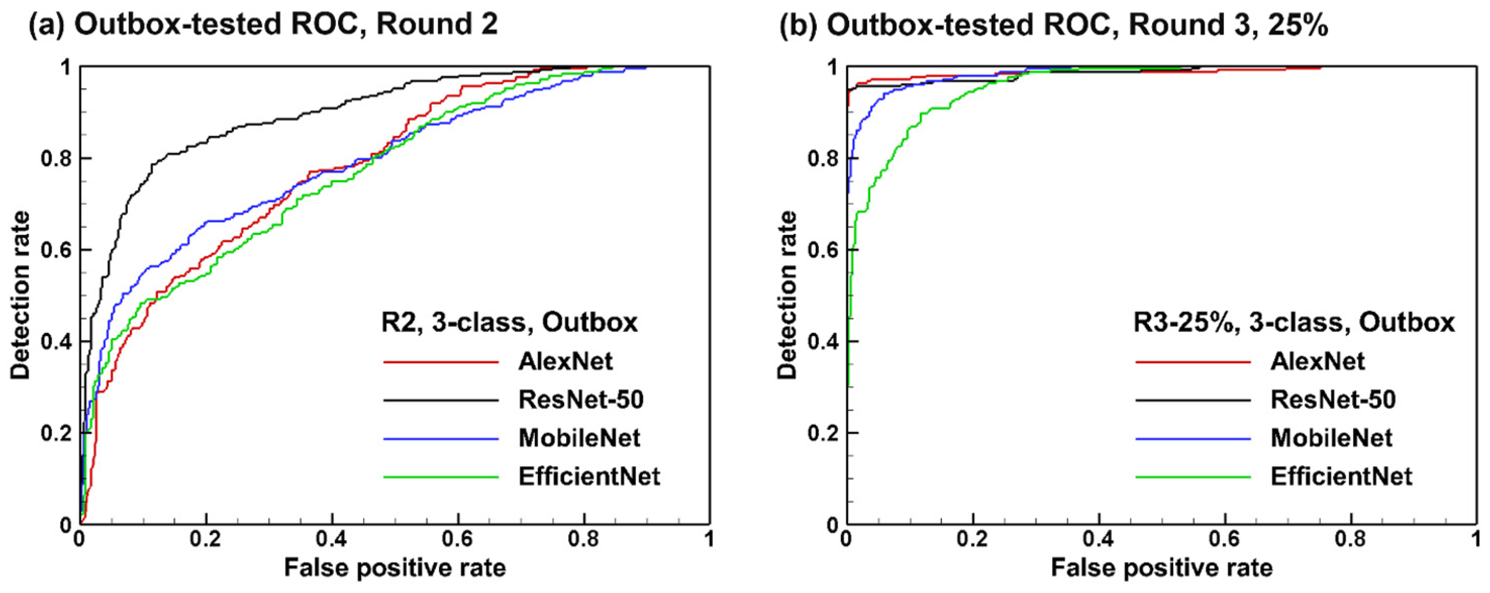
3.3.4. Outbox-Tested ROC Curves: Round 2 vs. 3
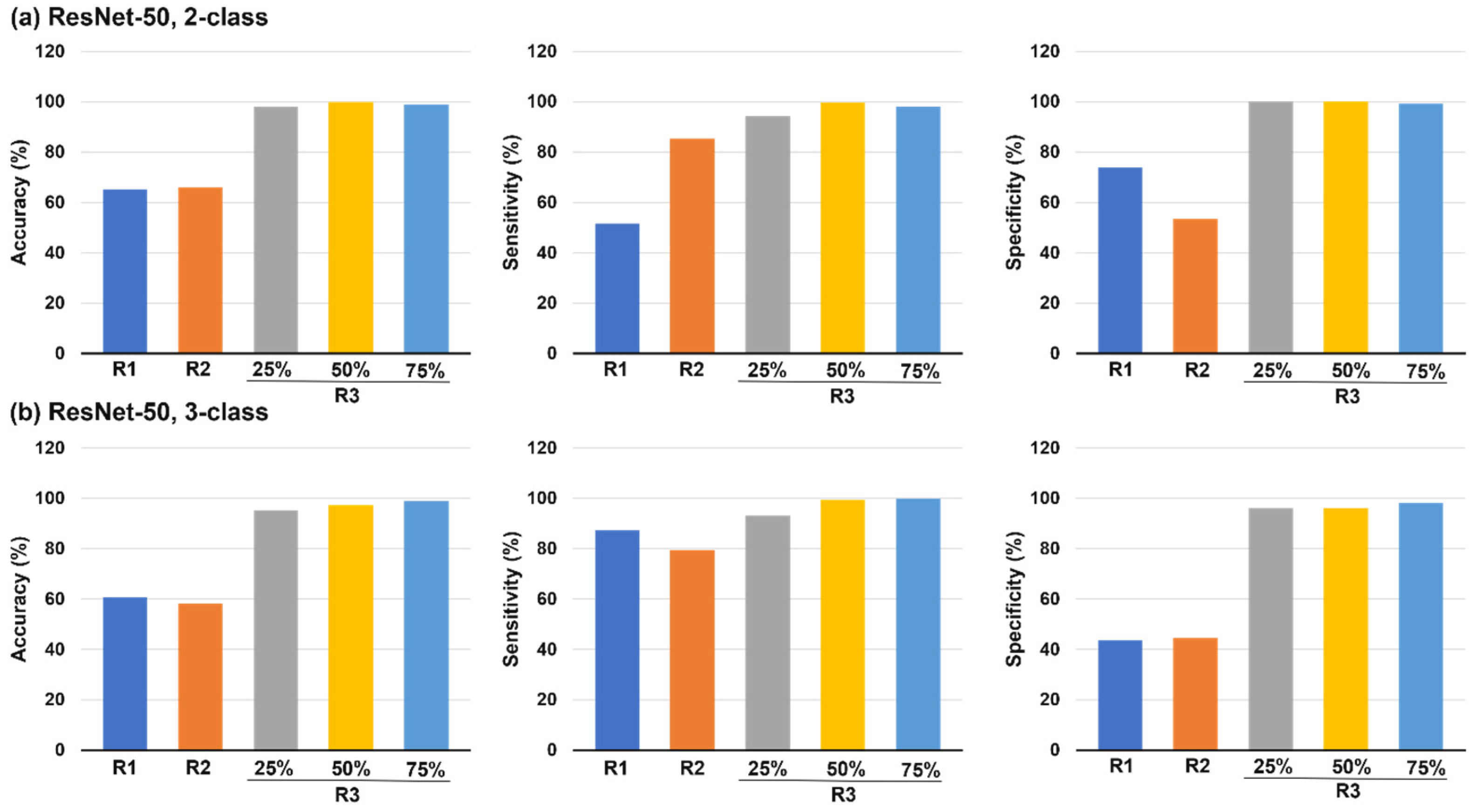
Figure 8 shows the ROC curves based on the Outbox dataset in Round 2 and Round 3. For a 3-class classification, there will be three piecewise ROC curves, and only ROC curves for normal vs. disease (i.e., D0 vs. D1 + D2) are shown here. Overall, all models performed better after adding 25% more Outbox data to the training set. Among the four models considered, ResNet-50 performed the best and EfficientNet the worst in both Rounds.

3.3.5. ResNet-50

The performance of the ResNet-50 on the Outbox testing dataset was evaluated systemically in Figure 9 when trained on five data sets with an increasing number of images. For both 2-class and 3-class classification tasks, an abrupt increase in accuracy was observed between R2 and R3-25%, which added 25% Outbox data (i.e., 20, 21, 22 L/min) into the training set; this indicated that the flow-associated features were predominant in classification. By comparison, the improvement in accuracy was incremental and insignificant in other scenarios (i.e., from R1 to R2, or from R3, 25% to 50% to 75%, left columns, Figure 9a,b), indicating that (1) features associated with throat-opening were less critical than flow-associated features and (2) a threshold amount of training images might exist for the model to reach feature saturation. Detailed classification results for R3-75% can be viewed in Table S3.
The sensitivity and specificity of ResNet-50 on five training sets are shown in the middle and right columns of Figure 9. For the 3-class classification, the sensitivity and specificity were calculated for the normal (D0). Overall, both metrics increased with training datasets that contained more images and more features, indicating that a network model would perform better in identifying both true positives and true negatives with continuous training. However, nonlinear variations were also observed from R1 to R2 (i.e., adding throat-related features) in both sensitivity (middle panel, Figure 9b) and specificity (left panel, Figure 9a). Note that the R1 training dataset (90% Base) did not contain throat-variation features, the above nonlinearity might result from the weight decrease of principle features due to the addition of non-critical features.

3.4. Model Performance on New Test Datasets (Inbox_dp and Outbox_dp)

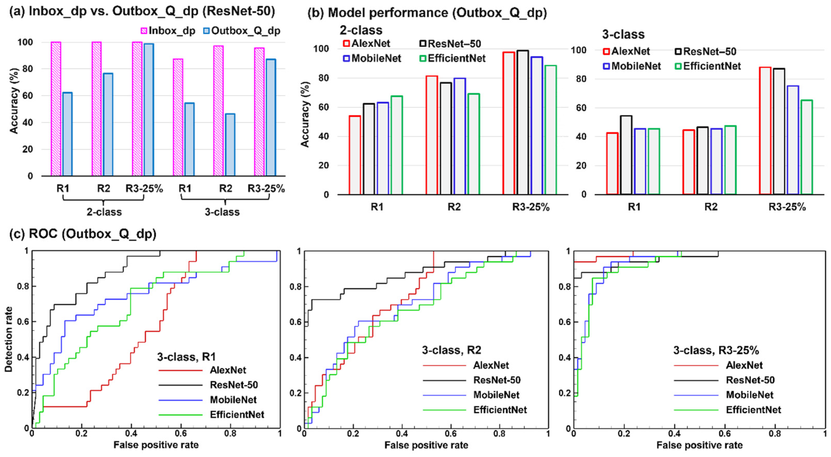
3.4.1. Inbox_dp vs. Outbox_Q_dp

Two new datasets, Inbox_dp and Outbox_dp, were prepared following the operating conditions listed in Figure 2c,d, respectively. Note that all models have never been trained on images with a particle size of 2.5, 4, 6, or 8 µm. Quantifying model performance on such datasets would evaluate the model’s interpolation capacity in terms of particle size.
Figure 10a compares the ResNet-50 performance tested on the new datasets. Note that the ResNet-50 model was trained three times separately on different training sets, i.e., Round 1 (R1), Round 2 (R2), and Round 3 with 25% Outbox images (R3-25%). All three sub-models achieved high accuracies on the Inbox_dp dataset, indicating that ResNet-50 could adequately interpolate the dp-associated features. Lower accuracies were achieved on the Outbox_Q_dp set, which contained features associated with both Q and dp. Thus, the flow rate Q might have a more dominant effect than the particle size on the classification performance. The accuracy increased from R1, to R2, to R3-25%, with R3-25% nearly reaching that tested on the Inbox_dp, which corroborated the benefits of continuous training/learning by the model to handle images that were similar but fell outside of the trained scope.

3.4.2. Different Models on Outbox_Q_dp

A comparison of different model performances on the Outbox_Q_dp dataset in different rounds is shown in Figure 10b. It is interesting to note that in Round 1, AlexNet and ResNet-50 had lower accuracy on the Outbox_Q_dp dataset for the 2-class classification task, while MobileNet and EfficientNet had higher accuracy. This may have been due to overfitting, which is a common issue in more complex neural network models. However, in Round 2, AlexNet and ResNet-50 regained their superiority.
For the 3-class classification task, all models had relatively low accuracies in Rounds 1 and 2, but a significant increase in accuracy occurred in Round 3–25%, where the training dataset included throat-variation information and outbox-flow information. This suggests that the relevance of the training data strongly correlates with the model’s performance.

3.4.3. ROC on Outbox_Q_dp

The ROC curves are compared in Figure 10c among different models in the 3-class classification on the Outbox_Q_dp. A significant improvement was observed for all models in R3-25% compared to R1 and R2. In R3-25%, both AlexNet and ResNet-50 performed significantly better than the two simpler models. However, ResNet-50 exhibited a more robust performance in all three rounds.

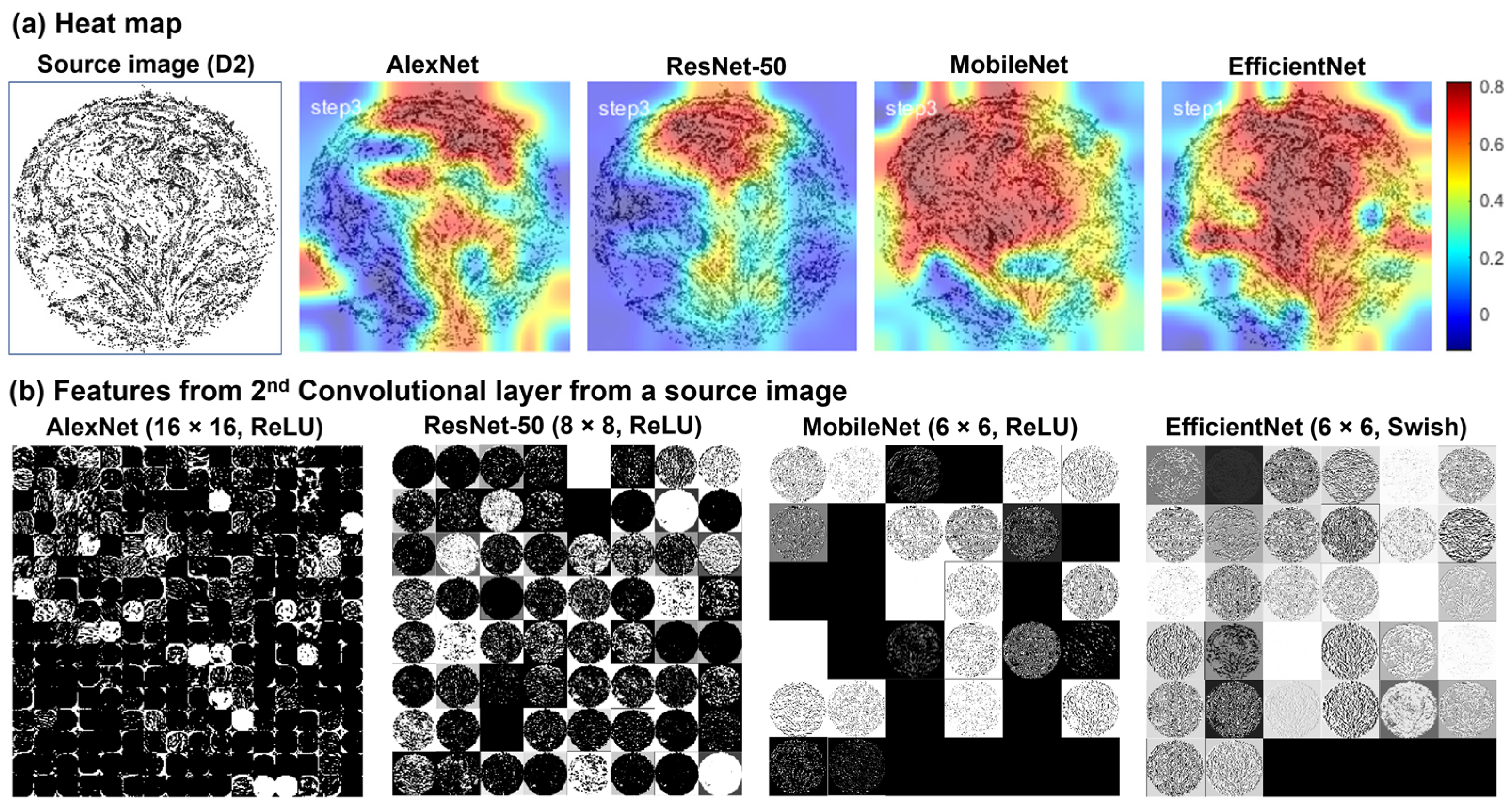
3.5. Heat Map and ReLU Features

To further evaluate the model’s capacity to capture the key features for classification, heat maps of a sample image from the four models were plotted in Figure 11a. The true class of this sample image was D2 (disease, 2nd stage, with 0.5, 15 L/min), with EfficientNet misclassifying it as D1 and the other three models classifying it correctly. By comparing the heat map in Figure 11 with the particle distributions from the diseased bronchioles in Figure 4a, we observed apparent similarities between these two, particularly for AlexNet and ResNet-50. This similarity suggested that the heat maps did provide a visual representation of which parts of the image were most influential in the classification decision. The heat maps from MobileNet and EfficientNet were less focused and covered a larger area, indicating either the inclusion of non-essential features or non-decisive weights for key features. For all models, we did not see heat spots in the background (4 corners).
Figure 11b shows the features from the sample image at the second convolutional layer. The first three networks used the ReLU (rectified Linear Unit) activation function, and the last one (EfficientNet) used a smoother Sigmoid-based Swish function. This might explain the presence of a large portion of black-out features in the first three compared to the smoother representations in EfficientNet. Image features became increasingly abstract and unrecognizable in deeper layers (not shown).

4. Discussion

4.1. Model Sensitivity to Small Airway Remodeling

The disease models in this study were generated by progressively constricting the G7-9 bronchioles in the left lower lobe. The bronchiolar diameters in these small airways are smaller than 1 mm, which is much smaller than the minimal nodule size that can be detected by current radiological techniques (i.e., 3–4 mm) [29]. It is essential that the selected CNN model can effectively detect and differentiate these disease-elicited disturbances in the exhaled aerosol images amidst a variety of confounding factors, which include flow rate, particle size, and throat opening. Specifically, the variations in throat opening were even larger than the disease-associated bronchiolar remolding. This study demonstrated that the CNN models, particularly ResNet-50, could effectively detect/differentiate disease-associated features from other features. One inherent advantage of CNN models is their ability to capture local patterns and spatial dependencies from input images with multiple layers, features, and dimensions. It is thus natural for a CNN model to differentiate input images according to any labeled features, even for weak disturbances from small airway remodeling, as in this study.

4.2. Geometrical, Breathing, and Aerosol Effects on Classification Decision

The breath tests that generate exhaled aerosol images can be affected by many other factors, like geometrical, breathing, and aerosol variants. Considering that CNN models are good at capturing features from individual factors, their effects on classification must result from their interactions with the target factor, here, the small airway constrictions. In this study, we observed that the variation in flow rate exerted a larger effect than particle size and throat variation on classification accuracy (Figure 7 and Figure 10). Adding images with flow rates of 20–22 L/min to the test dataset significantly lowered the classification accuracy (Outbox-testing in Figure 5, Table 2), while adding 25% of these images to the training dataset greatly improved the model performance (Figure 7b, Table S1). By comparison, relatively high classification accuracies were still achieved on new test images with particles of 2.5, 4, 6, and 8 µm (Figure 10a, Inbox_dp), indicating their weaker interactions with the airway constrictions. Likewise, adding images from throat variations Th1 and Th2 into the training dataset in R2 led to only limited improvements in the classification accuracy (Figure 7), suggesting a nonsignificant impact from this geometrical variation on classification decisions.
The finding that the flow rate played a more important role in the classification decision than the particle size and throat variation was consistent with the observations in Figure 4, where the particle distributions from the diseased bronchioles were more dependent on the flow rate than the particle size and throat variation. One reason was that the particle response time (τp = ρdp2/18 µ), despite being proportional to dp2, was still much smaller than the flow time from the disease site (G7-9) to the mouth opening. After a prompt adjustment to local flows, the particles mainly followed the bulk flow, whose dynamics within a given airway were mostly determined by the flow rate.

4.3. Model Evaluation and Continous Learning

In this study, four CNN models were compared in their ability to diagnose and stage small airway constrictions. The 2-class (normal vs. disease) classification accuracy was always higher than the corresponding 3-class (D0 vs. D1 vs. D2) classification (Table 2). The capacity of the model to classify images inside and outside the original design space was assessed. In doing so, each model was tested on three levels of data with decreasing similarities, with Level 1 being similar images as the training set (for validation purposes), Level 2 being unseen images within the same design space (i.e., Inbox, to evaluate the model’s interpolation capacity), and Level 3 being new images with dissimilarities (i.e., Outbox, to evaluate extrapolation capacity). This multi-level testing aimed to simulate the clinical applications more realistically, where test images from patients could be either within or outside the original training dataset. The results in this study (Table 2, Figure 5 and Figure 6) clearly show that, despite high validation accuracy in Level 1, the accuracy for Inbox images could be noticeably compromised and that for Outbox images could be remarkably lower, indicating a limited extrapolation capacity of the network model. For instance, the accuracy ranged from 46 to 61% for 3-class classification on the Outbox set, which was too low to be clinically applicable (Table 1). Thus, continuous learning was needed to ensure the high performance of the CNN-aided diagnostic/staging system.
With this objective in mind, each model was trained in three rounds, with Round 1 representing the original training dataset, Round 2 adding images with throat variations to the training set, and Round 3 adding a specific amount of Outbox images, as listed in Table 1. With the model being exposed to more new images, the classification accuracy also increased progressively (Table 3, Figure 7, Figure 8, Figure 9 and Figure 10). The similarity between the training and testing datasets strongly correlated with the model performance, as demonstrated by the low accuracies of R2-trained models vs. the high accuracies of the R3-trained models on the Outbox test dataset (Figure 7a vs. Figure 7b). It was also observed that ResNet-50 was the most robust of the four models considered. ResNet-50 excelled over the other three models when tested on both inbox and outbox images and for both diagnostic (2-class: normal vs. disease) and staging (3-class: D0, D1, D2) purposes.
The hyperparameters played a pivotal role in both the training process and the model’s performance. The MaxEpochs parameter, which dictates the number of complete passes through the training dataset, significantly influenced the training process. A larger value of MaxEpochs, such as 50 epochs used for AlexNet, resulted in improved model performance than using 30 epochs, albeit at the expense of increased computational time. Another key parameter is the initial learning rate. A smaller learning rate (0.0001) used for ResNet50 allowed the model to converge more finely to an optimal solution. In contrast, a higher rate (0.001) might accelerate learning, but with the risk of overshooting optimal solutions. Lastly, the MiniBatchSize parameter affected both the convergence speed and memory requirements during training. In this study, a larger batch size of 32 was used for MobileNet and EfficientNet, which resulted in faster training compared to a smaller batch size of 25.

4.4. Limitations

As an exploratory study, the exhaled aerosol images used in this study were not from human subjects but were generated using computational fluid-particle simulations in physiologically realistic airway models. Currently, no breath test has been conducted in humans, so there are no in vivo images for training/testing. Future in vitro breath tests will be carried out on 3D-printed mouth-lung replicas with normal and diseased airways. Regarding the validity of simulation-generated images, previous studies have demonstrated that physiology-based simulations could sufficiently reproduce in vivo conditions [43,44]. Two numerical limitations existed in current simulations: steady flows and rigid walls, which would alter the exhaled aerosol distributions [45,46,47,48,49]. However, the differences caused by other variables could still be captured, which was the basis for classification. Methodology-wise, this study can be further improved by considering a time series of exhaled aerosol images rather than the cumulative static images used in this study. A dynamic variation of bolus distribution/concentration vs. expiration time will presumably provide more information about airway structures and thus be more accurate in diagnosing/staging airway structural abnormalities [50,51,52,53].
It is noted that exhaled aerosols can be affected by many factors, such as airway motion, turbulence, intersubject variability, etc. A natural question is whether the proposed aerosol breath testing can still differentiate diseases under various compounding factors. Here we list five common questions surrounding the clinical applications of the proposed method: (1) How will the breath test be performed? (2) How can a classifier be developed when there is no record of aerosol images at the patient’s first visit? (3) How to minimize the compounding effects of geometrical and breathing variability among different patients? (4) What is the turbulent effect on model performance? and (5) how to tell the disease location from aerosol images? Detailed answers to these five questions were provided in Si and Xi [18], and interested readers can find more relevant information there.

5. Conclusions

This study explored the feasibility of using convolutional neural networks (CNN) to diagnose and stage obstructive lung diseases. Multiple-round and multi-class training/testing were conducted on exhaled aerosol images generated by physiology-based simulations in normal and diseased airways. Four CNN models, AlexNet, ResNet-50, MobileNet, and EfficientNet, were tested on their capacity to classify images inside and outside the design space (i.e., Inbox and Outbox), as well as the effect of continuous learning on their performance. Specific findings included:
(1)
All models showed reasonably high classification accuracy on inbox images; the accuracy decreased notably on outbox images, with the magnitude varying with models;
(2)
ResNet-50 was the most robust among the four models when tested on both inbox and outbox images and for both diagnostic (2-class: normal vs. disease) and staging (3-class: D0, D1, D2) purposes;
(3)
CNN models could detect small airway remodeling (<1 mm) amidst a variety of variants (including glottal aperture changes of larger magnitudes, i.e., 3 mm);
(4)
Variation in flow rate was observed to be more important than throat opening and particle size in classification decisions;
(5)
Continuous learning significantly improved classification accuracy, with the relevance of training data strongly correlating with model performance.

Supplementary Materials

The following supporting information can be downloaded at: https://www.mdpi.com/article/10.3390/jnt4030011/s1. Table S1: Round-3-25% performance comparison among models (AlexNet, ResNet-50, MobileNet, and EfficientNet) that were trained on (90% Base, Th1,2, and 25% Outbox) and tested on samples with decreasing similarities (Level 1, Inbox, Outbox) for both 2-class and 3-class classifications. Table S2: Round-3–50% performance comparison among models (AlexNet, ResNet-50, MobileNet, and EfficientNet) that were trained on (90% Base, Th1,2, and 50% Outbox) and tested on samples with decreasing similarities (Level 1, Inbox, Outbox) for both 2-class and 3-class classifications. Table S3: Round-3–75% performance comparison among models (AlexNet, ResNet-50, MobileNet, and EfficientNet) that were trained on (90% Base, Th1,2, and 75% Outbox) and tested on samples with decreasing similarities (Level 1, Inbox, Outbox) for both 2-class and 3-class classifications.

Author Contributions

Conceptualization, M.T., X.A.S. and J.X. (Jinxiang Xi); methodology, M.T., J.X. (Jensen Xi), K.T., X.A.S. and J.X. (Jinxiang Xi); software, M.T., K.T. and J.X. (Jinxiang Xi); validation, J.X. (Jensen Xi), K.T., X.A.S. and J.X. (Jinxiang Xi); formal analysis, M.T. and J.X. (Jinxiang Xi); investigation, J.X. (Jensen Xi), K.T., X.A.S. and J.X. (Jinxiang Xi); data curation, M.T.; writing—original draft preparation, M.T. and J.X. (Jinxiang Xi); writing—review and editing, J.X. (Jensen Xi), K.T. and X.A.S.; visualization, M.T. and J.X. (Jinxiang Xi); supervision, J.X. (Jinxiang Xi) All authors have read and agreed to the published version of the manuscript.

Funding

This research received no external funding.

Institutional Review Board Statement

Not applicable.

Informed Consent Statement

Not applicable.

Data Availability Statement

A companion paper that contains all images, itemized classification results, and Tables summarizing all data, has been submitted to MDPI Data.

Acknowledgments

Amr Seifelnasr at UMass Lowell Biomedical Engineering is gratefully acknowledged for editing and proofreading this manuscript.

Conflicts of Interest

The authors declare no conflict of interest.

References

  1. Darquenne, C. Aerosol deposition in health and disease. J. Aerosol Med. Pulm. Drug Deliv. 2012, 25, 140–147. [Google Scholar] [CrossRef] [Green Version]
  2. Xi, J.; Kim, J.; Si, X.A.; Corley, R.A.; Kabilan, S.; Wang, S. CFD modeling and image analysis of exhaled aerosols due to a growing bronchial tumor: Towards non-invasive diagnosis and treatment of respiratory obstructive diseases. Theranostics 2015, 5, 443–455. [Google Scholar] [CrossRef]
  3. Lee, D.Y.; Lee, J.W. Dispersion during exhalation of an aerosol bolus in a double bifurcation. J. Aerosol Sci. 2001, 32, 805–815. [Google Scholar] [CrossRef]
  4. Darquenne, C.; Prisk, G.K. The effect of aging on aerosol bolus deposition in the healthy adult lung: A 19-year longitudinal study. J. Aerosol Med. Pulm. Drug Deliv. 2020, 33, 133–139. [Google Scholar] [CrossRef]
  5. Schwarz, K.; Biller, H.; Windt, H.; Koch, W.; Hohlfeld, J.M. Characterization of exhaled particles from the human lungs in airway obstruction. J. Aerosol Med. Pulm. Drug Deliv. 2015, 28, 52–58. [Google Scholar] [CrossRef]
  6. Kohlhäufl, M.; Brand, P.; Rock, C.; Radons, T.; Scheuch, G.; Meyer, T.; Schulz, H.; Pfeifer, K.J.; Häussinger, K.; Heyder, J. Noninvasive diagnosis of emphysema. Aerosol morphometry and aerosol bolus dispersion in comparison to HRCT. Am. J. Respir. Crit. Care Med. 1999, 160, 913–918. [Google Scholar] [CrossRef]
  7. Verbanck, S.; Schuermans, D.; Paiva, M.; Vincken, W. Saline aerosol bolus dispersion. II. The effect of conductive airway alteration. J. Appl. Physiol. 2001, 90, 1763–1769. [Google Scholar] [CrossRef] [Green Version]
  8. Sturm, R. Aerosol bolus dispersion in healthy and asthmatic children-theoretical and experimental results. Ann. Transl. Med. 2014, 2, 47. [Google Scholar]
  9. Xi, J.; Kim, J.; Si, X.A.; Zhou, Y. Diagnosing obstructive respiratory diseases using exhaled aerosol fingerprints: A feasibility study. J. Aerosol Sci. 2013, 64, 24–36. [Google Scholar] [CrossRef]
  10. Anderson, P.J.; Dolovich, M.B. Aerosols as diagnostic tools. J. Aerosol Med. 1994, 7, 77–88. [Google Scholar] [CrossRef]
  11. Blanchard, J.D. Aerosol bolus dispersion and aerosol-derived airway morphometry: Assessment of lung pathology and response to therapy, Part 1. J. Aerosol Med. 1996, 9, 183–205. [Google Scholar] [CrossRef]
  12. Löndahl, J.; Jakobsson, J.K.; Broday, D.M.; Aaltonen, H.L.; Wollmer, P. Do nanoparticles provide a new opportunity for diagnosis of distal airspace disease? Int. J. Nanomed. 2017, 12, 41–51. [Google Scholar] [CrossRef] [Green Version]
  13. Inage, T.; Nakajima, T.; Yoshino, I.; Yasufuku, K. Early Lung Cancer Detection. Clin. Chest Med. 2018, 39, 45–55. [Google Scholar] [CrossRef]
  14. Roointan, A.; Ahmad Mir, T.; Ibrahim Wani, S.; Mati Ur, R.; Hussain, K.K.; Ahmed, B.; Abrahim, S.; Savardashtaki, A.; Gandomani, G.; Gandomani, M.; et al. Early detection of lung cancer biomarkers through biosensor technology: A review. J. Pharm. Biomed. Anal. 2019, 164, 93–103. [Google Scholar] [CrossRef]
  15. Blandin Knight, S.; Crosbie, P.A.; Balata, H.; Chudziak, J.; Hussell, T.; Dive, C. Progress and prospects of early detection in lung cancer. Open Biol. 2017, 7, 170070. [Google Scholar] [CrossRef] [Green Version]
  16. Dama, E.; Colangelo, T.; Fina, E.; Cremonesi, M.; Kallikourdis, M.; Veronesi, G.; Bianchi, F. Biomarkers and lung cancer early detection: State of the art. Cancers 2021, 13, 3919. [Google Scholar] [CrossRef]
  17. Eggert, J.A.; Palavanzadeh, M.; Blanton, A. Screening and early detection of lung cancer. Semin. Oncol. Nurs. 2017, 33, 129–140. [Google Scholar] [CrossRef]
  18. Si, X.A.; Xi, J. Deciphering exhaled aerosol fingerprints for early diagnosis and personalized therapeutics of obstructive respiratory diseases in small airways. J. Nanotheranostics 2021, 2, 94–117. [Google Scholar] [CrossRef]
  19. Xi, J.; Zhao, W.; Yuan, J.E.; Kim, J.; Si, X.; Xu, X. Detecting lung diseases from exhaled aerosols: Non-invasive lung diagnosis using fractal analysis and SVM classification. PLoS ONE 2015, 10, e0139511. [Google Scholar] [CrossRef] [Green Version]
  20. Xi, J.; Zhao, W. Correlating exhaled aerosol images to small airway obstructive diseases: A study with dynamic mode decomposition and machine learning. PLoS ONE 2019, 14, e0211413. [Google Scholar] [CrossRef] [Green Version]
  21. Xi, J.; Si, X.A.; Kim, J.; Mckee, E.; Lin, E.-B. Exhaled aerosol pattern discloses lung structural abnormality: A sensitivity study using computational modeling and fractal analysis. PLoS ONE 2014, 9, e104682. [Google Scholar] [CrossRef] [Green Version]
  22. Valverde, J.M.; Imani, V.; Abdollahzadeh, A.; de Feo, R.; Prakash, M.; Ciszek, R.; Tohka, J. Transfer learning in magnetic resonance brain imaging: A systematic review. J. Imaging 2021, 7, 66. [Google Scholar] [CrossRef]
  23. Ayana, G.; Dese, K.; Choe, S.W. Transfer learning in breast cancer diagnoses via ultrasound imaging. Cancers 2021, 13, 738. [Google Scholar] [CrossRef]
  24. Gao, Y.; Cui, Y. Deep transfer learning for reducing health care disparities arising from biomedical data inequality. Nat. Commun. 2020, 11, 5131. [Google Scholar] [CrossRef]
  25. Link, J.; Perst, T.; Stoeve, M.; Eskofier, B.M. Wearable sensors for activity recognition in ultimate frisbee using convolutional neural networks and transfer learning. Sensors 2022, 22, 2560. [Google Scholar] [CrossRef]
  26. Maray, N.; Ngu, A.H.; Ni, J.; Debnath, M.; Wang, L. Transfer learning on small datasets for improved fall detection. Sensors 2023, 23, 1105. [Google Scholar] [CrossRef]
  27. Xi, J.; Zhao, W.; Yuan, J.E.; Cao, B.; Zhao, L. Multi-resolution classification of exhaled aerosol images to detect obstructive lung diseases in small airways. Comput. Biol. Med. 2017, 87, 57–69. [Google Scholar] [CrossRef]
  28. Xi, J.; Wang, Z.; Talaat, K.; Glide-Hurst, C.; Dong, H.J.S. Numerical study of dynamic glottis and tidal breathing on respiratory sounds in a human upper airway model. Sleep Breath. 2018, 22, 463–479. [Google Scholar] [CrossRef] [Green Version]
  29. U.S. Preventive Services Task Force. Screening for Lung Cancer: US Preventive Services Task Force Recommendation Statement. JAMA 2021, 325, 962–970. [Google Scholar] [CrossRef]
  30. Talaat, M.; Si, X.A.; Dong, H.; Xi, J. Leveraging statistical shape modeling in computational respiratory dynamics: Nanomedicine delivery in remodeled airways. Comput. Methods Programs Biomed. 2021, 204, 106079. [Google Scholar] [CrossRef]
  31. Xi, J.; Talaat, M.; Si, X.A.; Chandra, S. The application of statistical shape modeling for lung morphology in aerosol inhalation dosimetry. J. Aerosol Sci. 2021, 151, 105623. [Google Scholar] [CrossRef]
  32. Krizhevsky, A.; Sutskever, I.; Hinton, G.E. Imagenet classification with deep convolutional neural networks. Commun. ACM 2017, 60, 84–90. [Google Scholar] [CrossRef] [Green Version]
  33. Xie, S.; Girshick, R.; Dollar, P.; Tu, Z.; He, K. Aggregated residual transformations for deep neural networks. In Proceedings of the 2017 IEEE Conference on Computer Vision and Pattern Recognition (CVPR), Honolulu, HI, USA, 21–26 July 2017; pp. 5987–5995. [Google Scholar]
  34. Loey, M.; Manogaran, G.; Taha, M.H.N.; Khalifa, N.E.M. Fighting against COVID-19: A novel deep learning model based on YOLO-v2 with ResNet-50 for medical face mask detection. Sustain. Cities Soc. 2021, 65, 102600. [Google Scholar] [CrossRef]
  35. Benali Amjoud, A.; Amrouch, M. Convolutional neural networks backbones for object detection. In Image and Signal Processing, Proceedings of the 9th International Conference, ICISP 2020, Marrakesh, Morocco, 4–6 June 2020; Springer: Berlin/Heidelberg, Germany, 2020; Volume 12119. [Google Scholar]
  36. Tan, M.; Le, Q. EfficientNet: Rethinking model scaling for convolutional neural networks. In Proceedings of the International Conference on Machine Learning, Long Beach, CA, USA, 10–15 June 2019. [Google Scholar]
  37. Tan, M.; Le, Q. Efficientnetv2: Smaller models and faster training. arXiv 2021, arXiv:2104.00298v00293. [Google Scholar]
  38. Howard, A.G.; Zhu, M.; Chen, B.; Kalenichenko, D.; Wang, W.; Weyand, T.; Andreetto, M.; Adam, H. Mobilenets: Efficient convolutional neural networks for mobile vision applications. arXiv 2017, arXiv:1704.04861. [Google Scholar]
  39. Sandler, M.; Howard, A.; Zhu, M.; Zhmoginov, A.; Chen, L.-C. Mobilenetv2: Inverted residuals and linear bottlenecks. In Proceedings of the IEEE Conference on Computer Vision and Pattern Recognition (CVPR), Salt Lake City, UT, USA, 18–23 June 2018; pp. 4510–4520. [Google Scholar]
  40. Bansal, N.; Aljrees, T.; Yadav, D.P.; Singh, K.U.; Kumar, A.; Verma, G.K.; Singh, T. Real-time advanced computational intelligence for deep fake video detection. Appl. Sci. 2023, 13, 3095. [Google Scholar] [CrossRef]
  41. Wang, Z.; Shi, Z.; Tong, J.; Gong, W.; Wu, Z. A detection method for impact point water columns based on improved YOLO X. AIP Adv. 2022, 12, 065011. [Google Scholar] [CrossRef]
  42. Michele, A.; Colin, V.; Santika, D.D. MobileNet convolutional neural networks and support vector machines for palmprint recognition. Procedia Comput. Sci. 2019, 157, 110–117. [Google Scholar] [CrossRef]
  43. Xiao, Q.; Stewart, N.J.; Willmering, M.M.; Gunatilaka, C.C.; Thomen, R.P.; Schuh, A.; Krishnamoorthy, G.; Wang, H.; Amin, R.S.; Dumoulin, C.L.; et al. Human upper-airway respiratory airflow: In vivo comparison of computational fluid dynamics simulations and hyperpolarized 129Xe phase contrast MRI velocimetry. PLoS ONE 2021, 16, e0256460. [Google Scholar] [CrossRef]
  44. Xi, J.; Kim, J.; Si, X.A.; Corley, R.A.; Zhou, Y. Modeling of inertial deposition in scaled models of rat and human nasal airways: Towards in vitro regional dosimetry in small animals. J. Aerosol Sci. 2016, 99, 78–93. [Google Scholar] [CrossRef]
  45. Si, X.; Talaat, M.; Xi, J. SARS CoV-2 virus-laden droplets coughed from deep lungs: Numerical quantification in a single-path whole respiratory tract geometry. Phys. Fluids 2021, 33, 023306. [Google Scholar]
  46. Talaat, M.; Si, X.; Tanbour, H.; Xi, J. Numerical studies of nanoparticle transport and deposition in terminal alveolar models with varying complexities. Med. One 2019, 4, e190018. [Google Scholar]
  47. Xi, J.; Talaat, M.J.N. Nanoparticle deposition in rhythmically moving acinar models with interalveolar septal apertures. J. Nanomater. 2019, 9, 1126. [Google Scholar] [CrossRef] [Green Version]
  48. Xi, J.; Si, X.A.; Dong, H.; Zhong, H. Effects of glottis motion on airflow and energy expenditure in a human upper airway model. Eur. J. Mech. B 2018, 72, 23–37. [Google Scholar] [CrossRef]
  49. Xi, J.; Walfield, B.; Si, X.A.; Bankier, A.A. Lung physiological variations in COVID-19 patients and inhalation therapy development for remodeled lungs. SciMedicine J. 2021, 3, 198–208. [Google Scholar] [CrossRef]
  50. Brand, P.; Rieger, C.; Schulz, H.; Beinert, T.; Heyder, J. Aerosol bolus dispersion in healthy subjects. Eur. Respir. J. 1997, 10, 460–467. [Google Scholar] [CrossRef] [Green Version]
  51. Ma, B.; Darquenne, C. Aerosol bolus dispersion in acinar airways—Influence of gravity and airway asymmetry. J. Appl. Physiol. 2012, 113, 442–450. [Google Scholar] [CrossRef] [Green Version]
  52. Lee, J.W.; Lee, D.Y.; Kim, W.S. Dispersion of an aerosol bolus in a double bifurcation. J. Aerosol Sci. 2000, 31, 491–505. [Google Scholar] [CrossRef]
  53. Wang, J.; Xi, J.; Han, P.; Wongwiset, N.; Pontius, J.; Dong, H. Computational analysis of a flapping uvula on aerodynamics and pharyngeal wall collapsibility in sleep apnea. J. Biomech. 2019, 94, 88–98. [Google Scholar] [CrossRef]
Figure 1. Computational mouth-lung models: (a) normal and diseased airway geometries with varying levels of bronchiolar constrictions in the left lower lung (i.e., D0, D1, and D2), as well as varying throat openings (i.e., Th0, Th1, Th2, and Th3); (b) a computational mesh with a fine, body-fitted prismatic mesh.
Jnt 04 00011 g001
Figure 2. Dataset architectures: (a) Diagram for data source from a systemic variation in the particle size (dp), respiration flow rate (Q), and throat opening (Th); (b) Baseline dataset (Base, 1080 images) with dp ranging 0.5–10 µm, Q ranging 10–19 L/min, and a normal throat opening (Th0), i.e., breath test design space; (c) Inbox dataset with both Q and dp falling within the design space, but either Q or dp differing from the baseline (i.e., Inbox_Q and Inbox_dp); (d) Outbox dataset with at least one of the three factors (i.e., dp, Q, Th) falling out of the design space, including outbox_Q, Outbox_Q_dp, Outbox_Th, and Outbox_Q_dp_Th. Explanations of the shape and colors of symbols were provided in text (see Section 2.3, 1st, 2nd, and 3rd paragraphs).
Jnt 04 00011 g002
Figure 3. Comparison of exhaled aerosol distributions between normal (a) and diseased lungs with mild (D1) and severe (D2) constrictions (b,c). Effects from particle size, flow rate, and throat constriction were considered.
Jnt 04 00011 g003
Figure 4. Comparison of exhaled aerosols released only from the disease-afflicted bronchioles during exhalation between normal lung (a) and (b) diseased lung D1, as well as (c) exhalation flows in disease-afflicted bronchioles. The black, green, and red color represents 0.5, 1.0, and 5 µm, respectively.
Jnt 04 00011 g004
Figure 5. Performance comparison on three test datasets with decreasing levels of similarity (Level 1, Inbox, and Outbox) in terms of accuracy, sensitivity, and specificity in Round 1 testing: (a) 2-class classification (normal vs. disease); (b) 3-class classification (D0 vs. D1 vs. D2).
Jnt 04 00011 g005
Figure 6. Performance comparison in 3-class classification among four network models in Round 1 testing: (a) Model accuracy, sensitivity, and specificity; (b) ROC (receiver operating characteristic) profiles.
Jnt 04 00011 g006
Figure 7. Classification accuracy on three test datasets (Level 1, Inbox, and Outbox) in terms of 2-class (normal vs. disease) and 3-class (D0 vs. D1 vs. D2) classifications in different rounds: (a) Round 2; (b) Round 3, 25% Outbox; (c) Round 3, 50% Outbox.
Jnt 04 00011 g007
Figure 8. Receiver operating characteristics (ROC) based on the Outbox test dataset: (a) Round 2 (R2); (b) Round 3, 25% Outbox (R3-25%).
Jnt 04 00011 g008
Figure 9. Comparison of ResNet-50 classification performance on the Outbox test dataset in different rounds: (a) 2-class; (b) 3-class.
Jnt 04 00011 g009
Figure 10. Performance of trained models on the new test dataset (Inbox_dp and Outbox_Q_dp, Figure 2a): (a) Inbox_dp vs. Outbox_Q_dp in 2-class and 3-class classifications; (b) Model effects in 2-class and 3-class classifications; (c) ROC in Rounds 1, 2, and 3.
Jnt 04 00011 g010
Figure 11. Image analysis: (a) Heat map; (b) Features from the 2nd ReLU layer. The true class of the image was D2, with EfficientNet misclassifying it as D1 and the other three models classifying it correctly.
Jnt 04 00011 g011
Table 1. Three-round training/testing procedures to evaluate the model capacity of interpolation, extrapolation, and continuous learning. These procedures will be tested in four models (AlexNet, ResNet-50, MobileNet, and EfficientNet) for both two-class (normal vs. disease) and three-class (D0 vs. D1, D2) classifications.
TrainingTesting
Level 1Level 2Level 3
Round 190% Base10% BaseInboxOutbox
Round 2: (plus 90% Base)Th1, Th210% BaseInboxOutbox
Round 3
(plus 90% Base,
and Th1, Th2)
25% Outbox10% BaseInboxOutbox
50% Outbox10% BaseInboxOutbox
75% Outbox10% BaseInboxOutbox
Table 2. Round-1 performance comparison among models (AlexNet, ResNet-50, MobileNet, and EfficientNet) that were trained on 90% Base and tested on samples with decreasing similarities (Level 1, Inbox, and Outbox) for both 2-class and 3-class classifications. AUC: area under the curve.
Round 1 2-Classes3-Classes
Network(%)Level 1InboxOutboxLevel 1InboxOutbox
AlexNetAccuracy10098.8858.4999.2483.5247.07
AUC10099.8963.8610010059.63
Specificity10099.1760.6198.9076.1132.83
Sensitivity10098.2855.1610098.8569.44
Precision10098.2847.1297.6266.6739.68
ResNet-50Accuracy10099.6365.1299.2482.7760.65
AUC10010075.1010099.9884.06
Specificity10010073.7498.9074.4443.69
Sensitivity10098.8551.5910010087.30
Precision10010055.5697.6265.4149.66
MobileNetAccuracy99.2496.6 360.1997.7373.4045.8
AUC99.7699.6867.5810099.0270.53
Specificity10099.4451.2696.7065.2826.26
Sensitivity97.5690.8074.2110090.2376.59
Precision10098.7549.2193.1855.6739.79
EfficientNetAccuracy96.9791.2061.2790.1570.2241.98
AUC10095.9867.1299.5796.1266.38
Specificity10097.2261.8789.0163.0629.55
Sensitivity90.2478.7460.3292.6885.0661.51
Precision10093.2050.1779.1752.6735.71
Table 3. Round-2 performance comparison among models (AlexNet, ResNet-50, MobileNet, and EfficientNet) that were trained on 90% Base and tested on samples with decreasing similarities (Level 1, Inbox, and Outbox) for both 2-class and 3-class classifications.
Round 2 2-Classes3-Classes
Network(%)Level 1InboxOutboxLevel 1InboxOutbox
AlexNetAccuracy98.6098.6968.0699.3080.1554.01
AUC99.9899.9479.5510099.9778.42
Specificity98.9099.1761.3698.9071.6735.10
Sensitivity98.0897.7078.5710097.7083.73
Precision98.0898.2756.4198.1162.5045.09
ResNet-50Accuracy99.3099.4465.9010091.0158.18
AUC10099.9984.5010099.9982.13
Specificity98.9010053.5410086.6744.70
Sensitivity10098.2885.3210010079.37
Precision98.1110053.8810078.3847.73
MobileNetAccuracy97.9095.8871.1495.1077.3454.48
AUC99.8999.3383.9610099.4079.35
Specificity98.9099.4462.1292.3168.3336.11
Sensitivity96.1588.5185.3210095.9883.33
Precision98.0498.7258.9088.1459.4345.36
EfficientNetAccuracy97.9093.0761.8893.068.7356.33
AUC99.8798.1971.1299.8197.0677.21
Specificity97.8096.9458.0891.2161.3948.48
Sensitivity98.8185.0667.8696.1583.9168.65
Precision96.2393.0850.7486.2151.2345.89
Disclaimer/Publisher’s Note: The statements, opinions and data contained in all publications are solely those of the individual author(s) and contributor(s) and not of MDPI and/or the editor(s). MDPI and/or the editor(s) disclaim responsibility for any injury to people or property resulting from any ideas, methods, instructions or products referred to in the content.

