Spectral Properties of Water Hammer Wave


1
Bureau of Watershed Management and Modeling, St. Johns River Water Management District, 4049 Reid Street, Palatka, FL 32177, USA
2
Jacobs Engineering Group, 112th Ave NE, Bellevue, WA 98004, USA
*
Author to whom correspondence should be addressed.
Appl. Mech. 2022, 3(3), 799-814; https://doi.org/10.3390/applmech3030047
Submission received: 13 April 2022
/
Revised: 22 June 2022
/
Accepted: 24 June 2022
/
Published: 1 July 2022
Abstract
:The prevention of excessive pressure build-up in pipelines requires a thorough understanding of water hammer phenomena. Using theoretical techniques, researchers have investigated this phenomenon and proposed productive solutions. In this article, we demonstrate a power spectral density approach on the pressure wave generated by water hammer in order to improve our understanding on the frequency domain approach as well as their fractal nature and complexity. This approach has the ability to explain some valuable attributes of the unsteady flow at a specific section, such as vulnerability and complexity that allow us more dynamic variables for effective analysis of pipe network design. Therefore, we aim to test a simple pipe system to simulate the proposed approach, which may offer useful physical information about pipeline network construction. The proposed method is expected to be beneficial and effective in acquiring a better understanding of the complicated features of unsteady flows as well as the sound acoustics within a pipe system and its design. In specific, our findings demonstrate the possibility for engineering design to comprehend the robustness, vulnerability, and complexity of pipe networks, as well as their sustainable construction.
1. Introduction: Water Hammer Phenomena
Most liquids are incompressible or barely compressible, so their volume remains constant under pressure. This is beneficial for hydraulic cylinders, but it can cause catastrophic pipe failure, called hydraulic transience or water hammer [1,2]. Given that we normally carry only a few ounces of water with us, it is important to emphasize its weight. Even in a single household’s pipe, water accumulates a substantial bulk in a city’s pipelines. All of this water is moving at a rapid rate through the pipe. Due to its incompressibility and elasticity, water cannot absorb the shock of a sudden stop, such as the closing of a valve. Perhaps concrete is used to reinforce the valve and pipe walls. Due to an abrupt change in momentum, a pressure spike occurs, which propagates as a shockwave through the pipe. Although the sound of water pounding on walls when a faucet is turned off or a washing machine is turned on may seem peculiar, this shockwave can be heard pounding in walls for large diameter pipelines. For example, a 100 km pipeline with a 1 m diameter contains around 80 MKg of water, which is a huge mass flow of water. As a result for closing a valve at the pipeline’s terminus, the pressure spike caused by the abrupt change in velocity may rupture the pipe or cause significant damage to other system components.
Due to this pressure, it may be more difficult to construct a pipeline or pipe network than it initially appears [3]; even slight pressure spikes can cause a system to malfunction. Some parameters affect the pressure profile of the water hammer pulse. Adjusting these variables can reduce forces that cause pipe damage. Slowing the flow of fluid through the pipe minimizes the impact. Flow velocity is affected by pipe diameter and flow rate. Due to a constant flow rate, the pipe diameter can be increased to minimize flow velocity. Smaller pipes are less expensive, however, the increased flow velocity might result in water hammer. Due to the constant diameter of the pipe, either the flow rate or the momentum change time can be decreased. Flywheels slow pumps instead of stopping them. Closing valves gradually reduces water hammer. Fluid sound velocity (wave celerity) describes the velocity at which a wave can travel through a conduit [1,2]. Fluid compressibility, pipe material, and whether or not the pipe is buried in a rigid structure determine wave speed. Water hammer can be eliminated by reflecting pressure waves by connecting a flexible PVC pipe to an anti-surge device with an air bladder. Water towers absorb variations in atmospheric pressure by permitting the free surface to rise and fall. As engineers, it is our responsibility to ensure that expensive infrastructure does not break when water is regulated, including forecasting and implementing procedures to avoid water pressure surge damage.
In the meantime, a stronger pressure pulsation is generated at the valve, causing a more complex water–structure interaction response in the water conveyance system [4,5,6,7]. This is extremely important in chemical refineries, power plant stations, and water supply systems. Accidents and fatalities are commonly associated with the term water hammer. For some, this term conjures up images of broken and bent piping, the loss of water supplies to cities, and deaths caused by water hammer. Literature from the past synthesizes the significance of water hammer phenomena and the associated risks in a variety of contexts, including chemical installations, power plant stations, and water supply [8].
Theoretical approaches such as power spectral density and entropy of time series are frequently used to quantify spectral properties in many disciplines. Recently, these approaches have been used in the hydrology field to study natural channel networks [9,10,11,12]. However, very little attention has been taken to the application of these approaches in the context of pipe water distribution and their physical phenomena.
2. Water Hammer Wave
2.1. Theory
The conventional momentum equation [1,2,13] can be used to explain the water hammer wave problem.
where force, density of water, initial velocity of water, and final velocity of water. As a result, when falls below , a negative force is created. Within a pipeline, this negative force creates a wave of increased pressure that propagates back toward the source of the flow and goes back and forth between the source and the destination. The wave speed, also known as celerity, is a function of the theoretical wave celerity (i.e., the pipe is considered to be rigid), which is given by
where theoretical wave celerity and bulk modulus of elasticity of fluid. However, in reality the pipe is elastic and the velocity of a pressure wave in an elastic fluid inside an elastic pipe is given by
where pipe diameter, thickness of pipe walls, and modulus of elasticity of pipe material. The maximum change in pressure created from water hammer in a pipeline is derived from the momentum Equation (1) and results in the following equation:
where change in pressure. Furthermore, when the time it takes for a valve to close is less than the pipe length divided by the wave celerity (i.e., ), this is called a rapid valve closing. Hence, the maximum pressure that will occur in the pipe is the original pressure within the pipe plus the change in pressure (Equation (5)).
This pressure variation will change in cycles at times equal to for a rapid interruption of the flow. Over time, the pressure wave will decrease due to pipe friction and damping. In other words, the pressure wave of water at a given point within a pipe oscillates, while overall steadily decreasing as time passes. Figure 1 depicts a relatively simple pipeline system in which a control valve abruptly blocks water flow from a reservoir. From the mathematical modeling point of view, if the coordinate x runs from the reservoir through the depicted pipeline of diameter d, we can consider the control valve at as an unsteady flow source. Initially, it supplies virtually no velocity fluctuation to the pipeline under the system pressure until the time reaches 0, and after that it gradually increases the velocity fluctuation until [14]. In general, pressure and flow velocity are independent variables in hydrodynamics, but they are dependent in linear acoustics [1,2,14].
The one-dimensional compressible fluid in the pipeline has the following continuity and momentum equations [14,15]:
where Darcy–Weisbach friction factor [1,2,14] and convective terms are neglected in most engineering applications because they are so small in comparison to the other terms, we also neglect the friction term’s effect, and we can simplify the above equations in the form of simple wave equations as below:
Equation (9) represents the wave form characteristics of a pressure wave induced by the water hammer effect. Consequently, a time series of the pressure amplitude () of the Fourier components can be represented as the spectrum of the wave form. Numerous studies have been conducted on the Fourier transformation of the pressure wave; however, the power spectral density approach and the concept of entropy have never been applied to the pressure wave caused by the water hammer effect.
In this study, the Fourier transform and fractal dimension of the pressure wave was adopted and analyzed to infer the instantaneous valve closure behavior as well as their wave complexity using the notion of entropy.
2.2. Pressure Losses in the Flow System
Pipe, elbow, and vessel exit contribute to the pressure losses of the flow system. The pressure loss is calculated by using Darcy–Weisbach Equation (10).
where L is the length of the pipe, d is the inner diameter of the pipe, is the density of the water, U is the velocity, and f is the friction factor. This friction factor (f) is a function of the surface roughness of the pipe, Reynolds number (), and the flow regime, i.e., laminar flow, transition zone, and turbulent flow [1,2,13]. Moody diagrams [1] are frequently used by engineers to depict the friction factor as a function of Reynolds number and flow regime. In order to investigate the effect of discharge on the spectrum of water hammer waves in pipes with constant length (1.5 m), diameter (OD 9.5 mm and ID 7.7 mm), and material, we conducted our experiment only under different discharge conditions.
3. Data Collection
3.1. Experimental Setup
This section will demonstrate our water hammer system for collecting data on water hammer waves. Figure 1 shows the schematic diagram of the water hammer system. Figure 2 and Figure 3 illustrate the components of the experiment’s equipment setup procedure. On the hydraulic bench, the setup includes a flow control valve in the pipe surge circuit, a water hammer valve, and a supply control valve (see details in [1]).
3.2. Procedure for Collecting Water Hammer Data
We began by closing the flow control valve on the hydraulic bench in the pipe surge circuit, followed by closing the supply control valve, and then by turning the black knob inward until it locked to open the fast-acting valve on the water hammer equipment. On the water hammer equipment, we closed the flow control valve at the end of the water hammer circuit and then activated the pump via the hydraulic bench switch. We gradually opened the hydraulic bench’s supply control valve and let the header tank fill to the level indicated by the transparent surge shaft’s water level; once the water reached the header tank’s overflow level, we opened the flow control valve in conjunction with the fast-acting valve. Following that, water was pumped through the test pipe, dislodging any trapped air. Water flowed consistently through the test pipe and out of the volumetric tank via the flexible exit tube. We adjusted the supply control valve on F1-10 as necessary to ensure that water returned to the sump tank via the overflow in a constant trickle [1].
We collected pressure wave data automatically using the C7MK11 application (water hammer software system). This software requires a virtual serial serial COM port on a USB port. For the specific details of this software and the data collection procedure, we refer readers to [1]. The software automatically generates graphs representing the pressure sensors and in the water hammer circuit (indicating atmospheric pressure). While water hammer pressure changes are significant in comparison to pipe surge pressures, they are so transient that they must be documented and viewed retrospectively rather than in real time. By fully opening the flow control and subsequently the fast-acting valve, we allow the water hammer circuit to settle. Thus, the surge shaft might provide information on the reservoir’s level. We ascertained that the clear return line is returning water to the sump tank. The flow control valve was adjusted as necessary to maintain a small overflow supply [1]. As indicated by a message in the lower left corner, the virtual oscilloscope was enabled once the water hammer exercise was installed on the computer. We navigated to the Operation section, clicked the GO icon in the top tool bar to initiate data logging, then pressed the trigger on the fast-acting valve within two seconds and waited for the data to be gathered and processed before saving them (see details in [1]).
3.3. Discharge Data Collection
4. Methods
4.1. The Essence of the Fourier Transform
The primary objective of this section is to explain the Fourier transform, a fundamental idea for comprehending waves, as well as its use in calculating power spectral density. This is the most important aspect for comprehending the idea of power spectral density used in this study. To show this concept, we can decompose the frequencies of a simple pressure wave and apply this knowledge to the comprehension of water hammer waves.
Figure 4 depicts a simple pressure wave and its progression in seconds. If we tracked the pressure wave around any source, it would oscillate at a certain frequency. When low and high frequency pressure waves are superimposed, the peaks can sometimes coincide, resulting in an increase in pressure, or they can cancel each other out. In other words, the pressure versus time graph is not a pure sine wave, and its complexity is increased by the addition of additional sine waves. The pressure over time is depicted in Figure 4 as a combination of two pure hypothetical pressure wave frequencies. The ultimate objective is to comprehend how the ’Fourier transform’ can separate complex pressure wave signals into distinct pure frequencies.
Consider a pure pressure wave signal with a period of 0–4.5 s (see Figure 4) to comprehend the concept. In this case, we can also consider a small rotating vector equal to the height of the signal at each time step. Each second, as depicted in Figure 4, the vector completes a half-cycle; thus, two seconds of time forwarding equals one circle rotation. Therefore, the initial signal can be separated into two frequencies: its three-cycle frequency and its half-rotation frequency. This second frequency is variable, enabling us to wrap it around faster or slower.
Each cycle in Figure 4 takes s, where the vertical lines represent the starting signal distance for a full-circle rotation. Consider this signal to be analogous to a metal wire, with this small dot representing the wire’s center of mass (). As the frequency of the signal varies, the wobbles and wraps differently. When the winding frequency and our signal frequency are identical, the is ideal. Now, it is possible to comprehend the transformation by considering the of each winding frequency. Specifically, we can consider the ’s x-coordinate. At zero frequency, the x-coordinate of the signal is large, but it decreases as it balances around the circle. Any intensity vs. time signal can be coiled and plotted in two dimensions to determine the effect of winding frequency on the original signal’s . This is the ’Fourier transform’ of our original signal; however, the complete Fourier transform can be calculated by using the x- and y-coordinates of the center of mass, which is typically located in the complex plane, to create a wound-up signal. This sophisticated method allows us to decompose a signal consisting of multiple frequencies. The mathematical expression for the process of creating a complex plane is Equation (11).
where this is a complex number with a real and an imaginary component. If e equals any number times , we can count that many counterclockwise units around a circle with unit radius, starting on the right. To denote one cycle per second rotation, we use ‘’ where t is the elapsed time. describes a 1-radius circle’s circumference. This mathematical formula captures winding a signal around a variable-frequency circle and tracking its . In this study, we aim to use the concept of power spectral density in the frequency domain of the water hammer wave discussed in the subsequent section.
4.2. Roughness in the Form of Fractals
In addition to the power spectral density approach, we intend to investigate the fractal dimension of pressure wave time series. Fractal is also a mathematical term for seemingly endlessly repeating patterns [17,18], however, fractals’ true nature and geometry remain abstruct. This section aims to provide a useful review of the concept of fractal dimension. Typically, fractals are assumed to be self-similar shapes, such as a von Koch snowflake or a Sierpinski triangle, etc. A simple shape can be used to generate more intricate shapes than its own self-similar patterns. Natural systems provide a physical foundation for fractals that can be used to calculate time series roughness. Mandelbrot demonstrated that self-similar patterns can be utilized to demonstrate a level of regularity in roughness. Fractals cannot be appropriately defined without the fractal dimension (D). The D value for the Sierpinski triangle is , the D value for the von Koch curve is , and the D value for the British coast is . In other words, any positive real integer may be utilized as a dimension for non-naturally sized forms. Example: a line is one-dimensional, a plane is two-dimensional, etc., here, ‘dimension’ is a mathematical term that refers exclusively to natural numbers. In addition to the formal concept of dimension, D can be defined in a more general way.
Self-similar geometries include a line, a square, a cube, and a Sierpinski triangle (Figure 5). A line can be represented by two half-sized lines, a square by four half-sized squares, and a cube by eight half-sized cubes. In addition, the Sierpinski triangle has three smaller replicas, each with a side length that is half that of the main triangle. Consequently, we can generally use the term ‘mass’ instead of ‘measure’. Consequently, the fractal dimension quantifies the scaling of an object’s mass. As demonstrated by the need for two copies of the similar mass to complete the line, halving the square mass reduces it by one-fourth. Similarly, halving a cube results in a mass reduction of one-eighth of the copies of the smaller cube and halving a Sierpinski triangle creates precisely three smaller triangles, reducing its mass by one-third. The fact that the mass of the line, square, and cube has been cut in half is remarkable. This exponent represents the shape’s dimensions. On the other hand, the dimension of the Sierpinski triangle is D, and can be calculated as . Likewise, the D value of the von Koch curve is . This D can also be accomplished in a commonly used, more general way.
In this study, we employ a method that can calculate D of pressure wave time series. For example, in this way, we can keep track of all grid squares that intersect the plane’s shape and count them to compute the area of contact between a disk and the grid, which should be proportional (see in Figure 5). In general, when plotted against the number of boxes intersected by the scaled disk, the scaling factor is a perfect parabola (see Figure 5). Scaling levels should be increased to accommodate a parabola, and the data are obtained by multiplying by a proportionality constant. Similarly, in the case of the UK coastline nearly as many boxes hit the coast as scaling factors are increased to . In other words, we can calculate the D by plotting the scaling factor against the number of boxes that touch the shoreline. In this study, the fractal dimension D was estimated using the box approach adopted from [20,21] to define the roughness of pressure waves [12].
4.3. Power Spectral Density in the Frequency Domain
Power spectral density () is a frequency response measurement of the signal intensity or amplitude. In general, it provides a standard method to capture how the energy in a signal is distributed across different frequencies. The of a discrete signal can be computed as the average magnitude of the Fourier transform squared [12], over a time interval, and expressed as follows:
where, is the discrete Fourier transform of and is its complex conjugate, and is the wave number [12,22,23,24]. We analyze this in the power-law domain across the frequency in the following form:
where is the power-law exponent of the and we refer to this as a proxy of the roughness of the wave signal, which is computed using the slope of the linear regression fitted to the estimated plotted on log–log scales [12,25].
4.4. Colors of Noise and Hurst Exponent
In physics, engineering, and many other fields, the color of noise refers to the power spectrum of a signal produced by a stochastic process, i.e., noise signal. They sound different to human ears as audio signals, and they have different textures as visuals. As a result, each application usually demands noise of a certain color. Some of the noise names have established definitions in specific areas, while others are either theoretical or poorly defined. Most of these definitions are under the assumption that a signal with a power spectral density per unit of bandwidth is proportional to and therefore they are defined as power-law noise. White noise, for example, is flat (i.e., ), while flicker or pink noise has , and Brownian noise has . Many time-dependent stochastic processes are known to exhibit noises with between 0 and 2. Brownian motion, in particular, has a power spectral density of , where is the diffusion coefficient [26]. In fractional Brownian motion, Hurst exponent H is also related to power spectral density with for subdiffusive processes () and for superdiffusive processes () [27,28].
The Hurst exponent is a metric for time series long-term memory. It has to do with time series autocorrelations and the pace at which they drop as the lag between pairs of values grows longer. It was established in hydrology for the purpose of calculating the optimum dam size for the Nile River’s fluctuating rain and drought conditions that had been studied over a long period of time [29]. In the fractal geometry discussed earlier, the generalized Hurst exponent has been denoted by H that directly relates to the fractal dimension, D, and is a measure of a data series’ ‘mild’ or ‘wild’ randomness [30]. It is a term used to describe long-range dependence, which quantifies a time series’ relative tendency to regress strongly to the mean or cluster in a certain direction. The value of H in the range 0.5∼1 implies a time series with long-term positive autocorrelation, whereas a value of 0∼0.5 indicates a time series with long-term flipping between high and low values in neighboring pairs. Furthermore, for self-similar time series, H is directly related to the fractal dimension, D, where , such that . The values of H vary between 0 and 1, with higher values indicating a smoother trend, less volatility, and less roughness [31]. The Hurst exponent and fractal dimension can be chosen independently for more generic time series or multi-dimensional processes, as the Hurst exponent represents structure over asymptotically longer periods, whereas the fractal dimension represents structure over asymptotically shorter periods [32].
4.5. Entropy: Approximate Entropy and Sample Entropy
Approximate entropy () is a form of Shannon entropy whose calculation involves a large amount of time series data; Steve M. Pincus developed this statistical technique to deal with the limitations of moment statistics by modifying an exact regularity statistic [33]. Although it was initially developed for the study of medical data, its applications later expanded to other fields [12,33,34,35].
The distance between two vectors and can be calculated using the maximum difference in their respective corresponding elements (see details in [35]).
where and and N is the number of data points in the pressure time series. For each vector , a measure that describes the similarity between the vector and all other vectors can be constructed using Equation (16), (see details in [35]).
where
The symbol r specifies a filtering level and is related to the standard deviation of the series. Finally, can be calculated by the following equation:
where
where m is the length of the compared patterns commonly known as the embedding dimension and r is the effective noise filter (see details in [36]).
Likewise, sample entropy () is another modified form of Shannon entropy that is used to determine the complexity of physical time series signals and to evaluate physical states. While is a measure of complexity similar to , it does not include self-similar patterns [35,37]. Both and algorithms are based on the calculation of conditional probabilities (see details in [36]), and the first two steps (14) and (15) are similar to . After the second step, is calculated for each template vector using Equation (20).
Then, summing over all template vectors can be written as Equation (21).
Similarly, for each template vector, we can calculate using Equation (22):
and the summing over all template vectors can be calculated using Equation (23).
Finally, can be calculated using Equation (24).
5. Results and Discussion
Pressure wave data caused by water hammer were extracted from the C7MK11 software setup (see details in Section 4) for four different initial flow rates (see Table 1). Table 1 shows the response of discharge in the power spectral properties as well as the entropy values for and points. In addition to the discharge, we have also collected the initial gauge pressure at and . From these discharges, other flow state parameters, such as the Reynolds number , can be calculated. The values of are 71,600, 141,875, 131,292, and 92,600, respectively. Table 1 only displays the best fitted slope (i.e., ) of in the power-law frequency domain (see details in Section 4). The subsequent paragraph describes the plot of in the power-law domain across the frequency.
Table 1 also shows the computed value of fractal dimension D and corresponding Hurst exponent H for different Q, and the value of H was calculated under the assumption of self-similar time series of pressure wave induced by water hammer.
Figure 6 and Figure 7 depict the power spectral density () plot of pressure wave data collected from pressure sensors and [1,2] for four different discharges, respectively. While both figures have the same shape, the log–log fitted slope () exhibits differences in the characteristics of the and pressure waves. As illustrated in Figure 6 and Figure 7, the value of the log–log fitted slope is greater for the wave sensor than for the wave sensor for all four discharges. This is because of applied forces that causes the water hammer effect. Although the correlation between the value and frequency is low (), the t-test indicates that the correlation is significant under the confidence interval [12,38]. From the perspective of colors of noise, we can say that both wave sensors exhibit near-flicker or pink noise, rather than purely random behavior. Additionally, this pink noise property supports our assumption about the wave equation presented in Equation (9). Additionally, the absolute value of the slope of for is slightly greater than that for , indicating that the wave has a slightly higher frequency variation than the wave, which is consistent with the behavior of the water hammer wave.
On the other hand, the relationship between the fractal dimension (D) and Hurst exponent (H) with described in the earlier sections demonstrates that the pressure wave for has a smoother temporal trend, less vulnerability, and less geometric roughness of time series than . This could be a useful property for understanding the behavior of pressure wave time series for pipe network vulnerability research and acoustics research for designing pipe networks. Furthermore, large amount of discharge may create a large D value and lower H value that creates more vulnerability inside the pipe.
Another important aspect of the pressure wave induced by the water hammer is the complexity of their time series. In this regard, we have computed the complexity based on the notion of entropy. The computed value of the complexity based on and is presented in Table 1. These two values provide us with a quantitative sense of the complexity of the pressure wave series for and . Additionally, and exhibit greater complexity in the presence of than in the presence of , despite their reverse vulnerability relation. These arguments imply that the pipe is less likely to break at the far point than at the near point of the hammer, due to the fact that the near point has a higher strength of variation and complexity of pressure wave induced by water hammer than the far point.
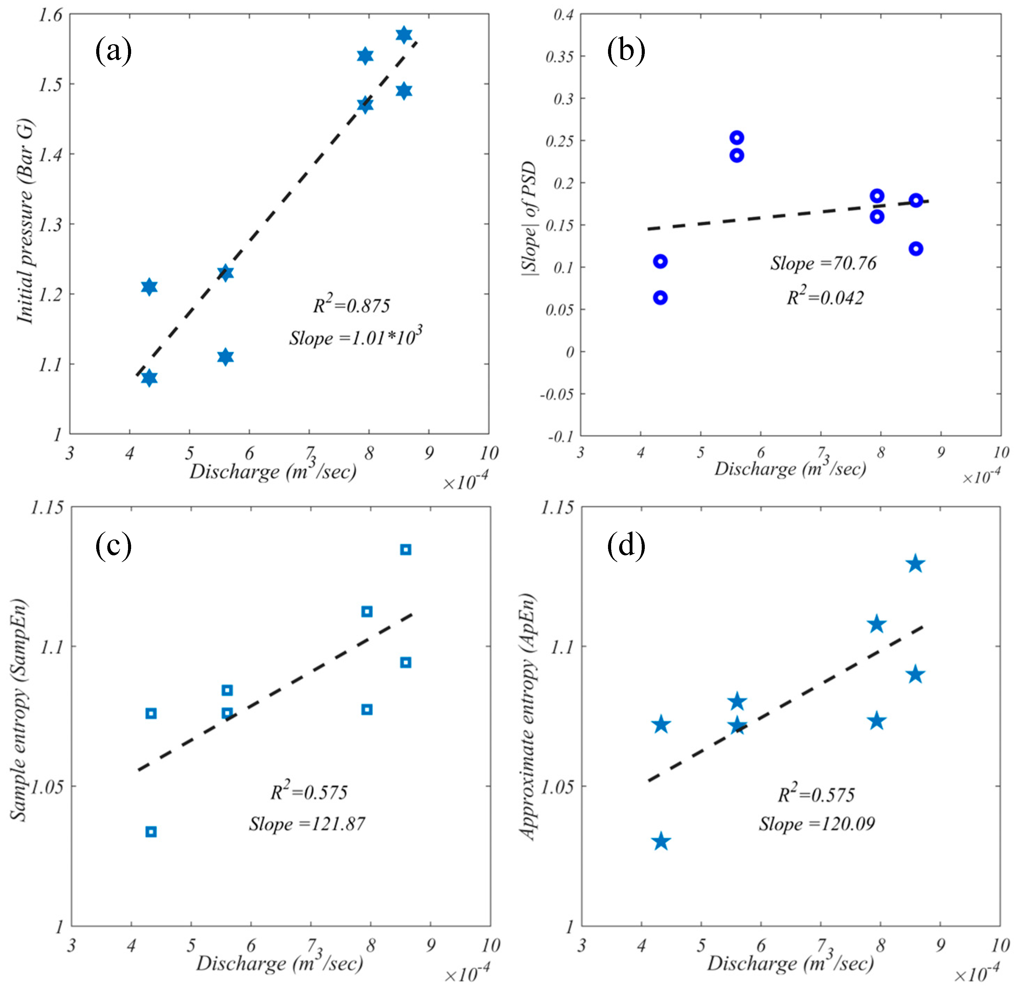
Figure 8a–d illustrate the effect of discharge on hydraulic properties and our proposed metric. As discharge increases, the gauge pressure at and increases significantly and linearly. In addition, the gauge pressure at is greater than that at due to the direction of flow (Figure 8a). In addition to other metrics, increases linearly with discharge (Figure 8b), consistent with the gauge pressure, and the value of for is greater than due to the damping effect or head loss [1,2,3,13].
Figure 8c–d illustrate the response of discharge on the complexity of a pressure wave induced by the water hammer. Specifically, complexity obtained from both and increases linearly with discharge significantly, which is consistent with previous studies [9]. However, complexity obtained from does not include self-similar patterns as does [37].
From the above discussion, we can argue that the proposed method may be beneficial for investigating the robustness, vulnerability, and complexity of pipe networks [3], especially for water distribution purposes.
6. Concluding Remarks
In this study, using power spectral density, the fractal dimension, and entropy approach, we have demonstrated useful spectral properties of pressure waves induced by the water hammer effect. The main results of this study can be summarized as follows:
- We explain how the notion of power spectral density can be implemented to understand the behavior of pressure waves generated by the water hammer effect and how the strength of variation is related to the flow rate.
- We propose a method for calculating the fractal behavior of pressure wave time series induced by the water hammer effect. This method may be used to investigate acoustics and design pipe networks.
- We also describe how the concept of entropy can be used to calculate the complexity of a water hammer-induced pressure wave.
- We demonstrate that the response of discharge through the pipe is proportional to the complexity of the pressure wave generated by the water hammer effect.
Our findings may assist in comprehending the robustness, vulnerability, and complexity of pressure waves induced by the water hammer effect, which has implications for the engineering design and sustainable construction of pipe networks.
Author Contributions
S.S. conducted the research, wrote the initial draft, and analyzed the results. T.S. assisted in the data collection for water hammer and provided feedback on the interpretation of the results. Each author contributed to the manuscript’s preparation. All authors have read and agreed to the published version of the manuscript.
Funding
This research received no external funding.
Institutional Review Board Statement
Not applicable.
Informed Consent Statement
Not applicable.
Data Availability Statement
The data for this study were gathered at the University of Central Florida’s hydraulics lab as part of undergraduate teaching, student homework, and an IAHR UCF student chapter volunteer demonstration of hydraulics. On reasonable request, the data can be made available.
Acknowledgments
Conflicts of Interest
The authors declare no conflict of interest.
References
- Sarker, S. Hydraulics Lab Manual. engrXiv 2021. [Google Scholar] [CrossRef]
- Sarker, S. A Short Review on Computational Hydraulics in the context of Water Resources Engineering. Open J. Model. Simul. 2022, 10, 1–31. [Google Scholar] [CrossRef]
- Sarker, S. Water Distribution (Pipe) Network Analysis with WaterCAD. Int. J. Eng. Dev. Res. IJEDR 2021, 9, 149–153. [Google Scholar]
- Guo, Q.; Zhou, J.; Li, Y.; Guan, X.; Liu, D.; Zhang, J. Fluid-structure interaction response of a water conveyance system with a surge chamber during water hammer. Water 2020, 12, 1025. [Google Scholar] [CrossRef] [Green Version]
- Cook, S.S. Erosion by water-hammer. Proc. R. Soc. Lond. Ser. A Contain. Pap. Math. Phys. Character 1928, 119, 481–488. [Google Scholar]
- Kandil, M.; Kamal, A.; El-Sayed, T. Effect of pipematerials on water hammer. Int. J. Press. Vessel. Pip. 2020, 179, 103996. [Google Scholar] [CrossRef]
- Azoury, P.; Baasiri, M.; Najm, H. Effect of valve-closure schedule on water hammer. J. Hydraul. Eng. 1986, 112, 890–903. [Google Scholar] [CrossRef]
- Leishear, R. Fluid Mechanics, Water Hammer, Dynamic Stresses, and Piping Design; ASME Press: New York, NY, USA, 2013. [Google Scholar] [CrossRef] [Green Version]
- Ranjbar, S.; Singh, A. Entropy and intermittency of river bed elevation fluctuations. J. Geophys. Res. Earth Surf. 2020, 125, e2019JF005499. [Google Scholar] [CrossRef]
- Sarker, S.; Veremyev, A.; Boginski, V.; Singh, A. Critical nodes in river networks. Sci. Rep. 2019, 9, 11178. [Google Scholar] [CrossRef] [Green Version]
- Sarker, S.; Veremyev, A.; Boginski, V.; Singh, A. Spectral Properties of River Networks. AGUFM 2019, 2019, EP51C–2107. [Google Scholar]
- Sarker, S. Investigating Topologic and Geometric Properties of Synthetic and Natural River Networks Under Changing Climatic. Ph.D. Thesis, University of Central Florida, Orlando, FL, USA, 2021. Available online: https://stars.library.ucf.edu/etd2020/965 (accessed on 20 December 2021).
- Sarker, S. Essence of MIKE 21C (FDM Numerical Scheme): Application on the River Morphology of Bangladesh. Open J. Model. Simul. 2022, 10, 88–117. [Google Scholar] [CrossRef]
- Lee, J.S.; Kim, B.K.; Lee, W.R.; Oh, K.Y. Analysis of water hammer in pipelines by partial fraction expansion of transfer function in frequency domain. J. Mech. Sci. Technol. 2010, 24, 1975–1980. [Google Scholar] [CrossRef]
- Reza, A.A.; Sarker, S.; Asha, S.A. An Application of 1-D Momentum Equation to Calculate Discharge in Tidal River: A Case Study on Kaliganga River. Tech. J. River Res. Inst. 2014, 2, 77–86. [Google Scholar]
- Sanderson, G. But what is the Fourier Transform? A visual introduction. 3Blue1Brown. 2018. Available online: https://www.youtube.com/watch?v=r6sGWTCMz2k (accessed on 12 April 2022).
- Rodriguez-Iturbe, I.; Rinaldo, A. Fractal River Basins: Chance and Self-Organization; Cambridge University Press: Cambridge, UK, 2001. [Google Scholar]
- Mandelbrot, B.B. The Fractal Geometry of Nature/Revised and Enlarged Edition; Freeman and Co.: New York, NY, USA, 1983. [Google Scholar]
- Sanderson, G. Fractals are typically not self-similar. 3Blue1Brown. 2017. Available online: https://www.youtube.com/watch?v=gB9n2gHsHN4 (accessed on 12 April 2022).
- Bhatt, S.; Dedania, H.; Shah, V.R. Fractal dimensional analysis in financial time series. Int. J. Financ. Manag. 2015, 5, 57–62. [Google Scholar] [CrossRef]
- Han. Fractal Volatility of Financial Time Series; MATLAB Central File Exchange: Natick, MA, USA, 2022. [Google Scholar]
- Stoica, P.; Moses, R.L. Spectral Analysis of Signals; Pearson Prentice Hall: Upper Saddle River, NJ, USA, 2005. [Google Scholar]
- Stull, R.B. An Introduction to Boundary Layer Meteorology; Springer Science & Business Media: Berlin/Heidelberg, Germany, 2012; Volume 13. [Google Scholar]
- Gardner, W.A.; Robinson, E.A. Statistical Spectral Analysis—A Nonprobabilistic Theory; Prentice-Hall, Inc.: Upper Saddle River, NJ, USA, 1989. [Google Scholar]
- Pilgram, B.; Kaplan, D.T. A comparison of estimators for 1f noise. Phys. D Nonlinear Phenom. 1998, 114, 108–122. [Google Scholar] [CrossRef]
- Norton, M.P.; Karczub, D.G. Fundamentals of Noise and Vibration Analysis for Engineers; Cambridge University Press: Cambridge, UK, 2003. [Google Scholar]
- Krapf, D.; Lukat, N.; Marinari, E.; Metzler, R.; Oshanin, G.; Selhuber-Unkel, C.; Squarcini, A.; Stadler, L.; Weiss, M.; Xu, X. Spectral content of a single non-Brownian trajectory. Phys. Rev. X 2019, 9, 011019. [Google Scholar] [CrossRef] [Green Version]
- Krapf, D.; Marinari, E.; Metzler, R.; Oshanin, G.; Xu, X.; Squarcini, A. Power spectral density of a single Brownian trajectory: What one can and cannot learn from it. New J. Phys. 2018, 20, 023029. [Google Scholar] [CrossRef]
- Hurst, H.E. Long-term storage capacity of reservoirs. Trans. Am. Soc. Civ. Eng. 1951, 116, 770–799. [Google Scholar] [CrossRef]
- Mandelbrot, B.B.; Hudson, R.L. The (Mis)behavior of Markets: A Fractal View of Risk, Ruin, and Reward; Basic Books: New York, NY, USA, 2005. [Google Scholar]
- Mandelbrot, B.B. Self-affine fractals and fractal dimension. Phys. Scr. 1985, 32, 257. [Google Scholar] [CrossRef]
- Gneiting, T.; Schlather, M. Stochastic models that separate fractal dimension and the Hurst effect. SIAM Rev. 2004, 46, 269–282. [Google Scholar] [CrossRef] [Green Version]
- Pincus, S.M. Approximate entropy as a measure of system complexity. Proc. Natl. Acad. Sci. USA 1991, 88, 2297–2301. [Google Scholar] [CrossRef] [PubMed] [Green Version]
- Pincus, S.; Kalman, R.E. Irregularity, volatility, risk, and financial market time series. Proc. Natl. Acad. Sci. USA 2004, 101, 13709–13714. [Google Scholar] [CrossRef] [PubMed] [Green Version]
- Sarker, S.; Sarker, T.; Raihan, S.U. Comprehensive Understanding of the Planform Complexity of the Anastomosing River and the Dynamic Imprint of the River’s Flow: Brahmaputra River in Bangladesh. Preprints 2022. [Google Scholar] [CrossRef]
- Delgado-Bonal, A.; Marshak, A.; Yang, Y.; Holdaway, D. Analyzing changes in the complexity of climate in the last four decades using MERRA-2 radiation data. Sci. Rep. 2020, 10, 922. [Google Scholar] [CrossRef]
- Richman, J.S.; Moorman, J.R. Physiological time-series analysis using approximate entropy and sample entropy. Am. J. Physiol. Heart Circ. Physiol. 2000, 278, 6. [Google Scholar] [CrossRef] [Green Version]
- Sarker, S. Understanding the Complexity and Dynamics of Anastomosing River Planform: A Case Study of Brahmaputra River in Bangladesh. In Proceedings of the AGU 2021 Fall Meeting, New Orleans, LA, USA, 28 November 2021. [Google Scholar] [CrossRef]
- Hillhouse, G. What is Water Hammer? Practical Engineering. 2017. Available online: https://practical.engineering/blog/2018/7/24/what-is-a-water-hammer (accessed on 12 April 2022).
Figure 1.
The diagram of a water hammer system, (a) schematic and (b) Armfield laboratory apparatus [1].
Figure 1.
The diagram of a water hammer system, (a) schematic and (b) Armfield laboratory apparatus [1].

Figure 2.
Laboratory water hammer system [1].
Figure 2.
Laboratory water hammer system [1].

Figure 3.
Components associated with the water hammer effect [1].
Figure 3.
Components associated with the water hammer effect [1].

Figure 4.
Illustration of the Fourier transformation, (a) frequency decomposition example, (b) original signal, (c) transformation from time to frequency domain, and (d) winding frequency example [16].
Figure 4.
Illustration of the Fourier transformation, (a) frequency decomposition example, (b) original signal, (c) transformation from time to frequency domain, and (d) winding frequency example [16].

Figure 5.
(a) Analogy of fractal dimensions with shape dimensions and (b) scale-wide generalization of fractal dimensions for various shapes [19].
Figure 5.
(a) Analogy of fractal dimensions with shape dimensions and (b) scale-wide generalization of fractal dimensions for various shapes [19].
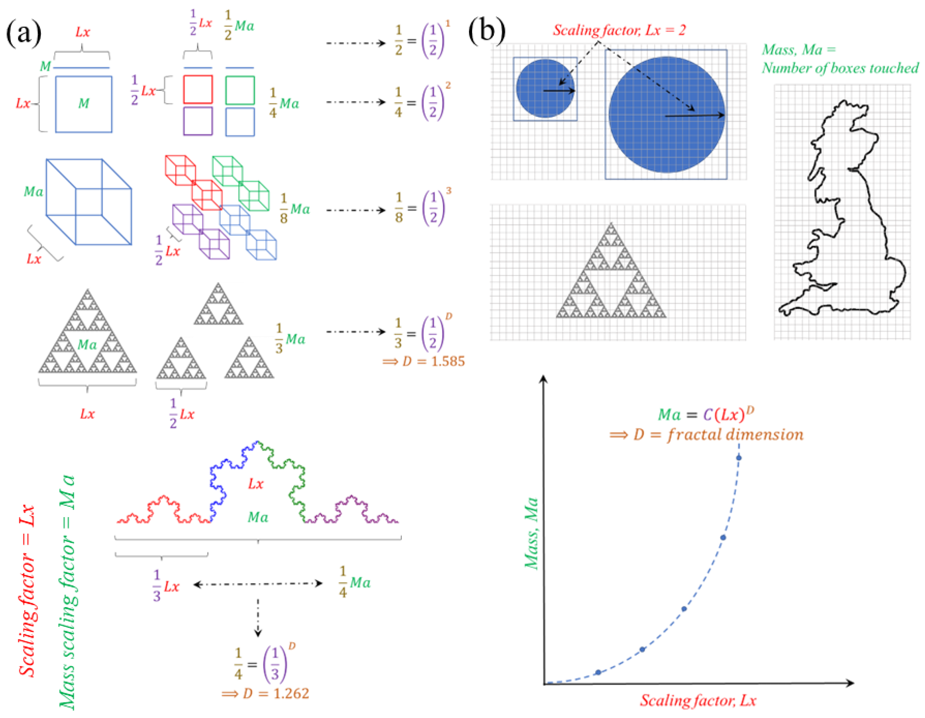
Figure 6.
Power spectral density across frequency for four different discharges, (a) Trial 1, (b) Trial 2, (c) Trial 3, and (d) Trial 4 for point , where slope of (see details in (13)). The and numerical values are displayed within each subplot.
Figure 6.
Power spectral density across frequency for four different discharges, (a) Trial 1, (b) Trial 2, (c) Trial 3, and (d) Trial 4 for point , where slope of (see details in (13)). The and numerical values are displayed within each subplot.

Figure 7.
Power spectral density across frequency for four different discharges, (a) Trial 1, (b) Trial 2, (c) Trial 3, and (d) Trial 4 for point , where slope of (see details in (13)). The and numerical values are displayed within each subplot.
Figure 7.
Power spectral density across frequency for four different discharges, (a) Trial 1, (b) Trial 2, (c) Trial 3, and (d) Trial 4 for point , where slope of (see details in (13)). The and numerical values are displayed within each subplot.
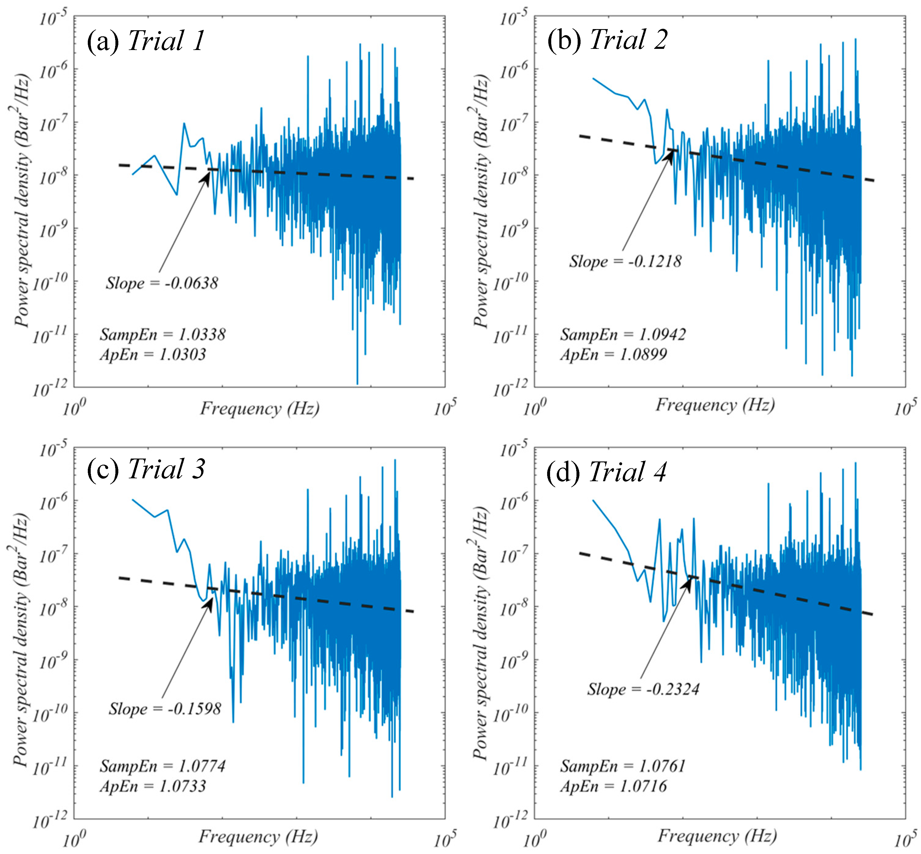
Figure 8.
Response of discharge, Q (m/sec), on (a) static gauge pressure, (b) absolute value of , (c) sample entropy , and (d) approximate entropy .
Figure 8.
Response of discharge, Q (m/sec), on (a) static gauge pressure, (b) absolute value of , (c) sample entropy , and (d) approximate entropy .

Table 1.
The outcomes of the experiment.
| Q = V/t m/s | Static Bar | Time (t) sec | |||||
|---|---|---|---|---|---|---|---|
| D | |||||||
| 0.000433 | 1.21 | −0.1068 | 1.076 | 1.072 | 1.8688 | 0.1312 | 46.2 |
| 0.000858 | 1.57 | −0.1791 | 1.1346 | 1.1295 | 1.8807 | 0.1193 | 23.3 |
| 0.000794 | 1.54 | −0.1844 | 1.1125 | 1.1079 | 1.8710 | 0.1290 | 25.2 |
| 0.00056 | 1.23 | −0.2534 | 1.0843 | 1.0802 | 1.8522 | 0.1478 | 35.7 |
| Q = V/t m/s | Static Bar | Time (t) sec | |||||
| D | |||||||
| 0.000433 | 1.08 | −0.0638 | 1.0338 | 1.0303 | 1.855 | 0.1450 | 46.2 |
| 0.000858 | 1.49 | −0.1218 | 1.0942 | 1.0899 | 1.8562 | 0.1438 | 23.3 |
| 0.000794 | 1.47 | −0.1598 | 1.0774 | 1.0733 | 1.8471 | 0.1529 | 25.2 |
| 0.00056 | 1.11 | −0.2324 | 1.0761 | 1.0716 | 1.830 | 0.1700 | 35.7 |
Publisher’s Note: MDPI stays neutral with regard to jurisdictional claims in published maps and institutional affiliations. |
© 2022 by the authors. Licensee MDPI, Basel, Switzerland. This article is an open access article distributed under the terms and conditions of the Creative Commons Attribution (CC BY) license (https://creativecommons.org/licenses/by/4.0/).
Share and Cite
MDPI and ACS Style
Sarker, S.; Sarker, T. Spectral Properties of Water Hammer Wave. Appl. Mech. 2022, 3, 799-814. https://doi.org/10.3390/applmech3030047
AMA Style
Sarker S, Sarker T. Spectral Properties of Water Hammer Wave. Applied Mechanics. 2022; 3(3):799-814. https://doi.org/10.3390/applmech3030047
Chicago/Turabian StyleSarker, Shiblu, and Tonmoy Sarker. 2022. "Spectral Properties of Water Hammer Wave" Applied Mechanics 3, no. 3: 799-814. https://doi.org/10.3390/applmech3030047