System Identification and Dynamic Analysis of the Propulsion Shaft Systems Using Response Surface Optimization Technique

Abstract

Marine vessels rely heavily on propeller shaft systems to adjust the engine torque and propeller thrust. However, these systems are subjected to various dynamic excitations during operation, such as transverse, longitudinal, and torsional excitations. These excitations can arise from factors like non-uniform stern flow fields, misaligned components, and the whirling motion of the shafts, which can affect the integrity and reliability of the vehicle. To analyze the dynamic response of the propulsion shaft system and ensure its reliability, numerical/analytical models are currently in practice. The finite element method (FEM) is a popular choice, but uncertainties in bearings and connectors stiffness lead to inaccuracies in the Finite Element model, resulting in significant differences between the experimental and theoretical models. This paper proposes the response surface optimization (RSO) technique to estimate unknown bearing stiffness in the propulsion shaft system. The experimental model of the propeller shaft system is constructed using steady-state response with step sine excitation. The RSO technique is then used to update the natural frequencies and vibration amplitude of the FE (Finite Element) model. The updated model shows less than a 10% difference in natural frequencies and vibration amplitude compared to the experimental model, demonstrating that the proposed technique is an efficient tool for marine shaft dynamic analysis.

1. Introduction

The propulsion shaft system is one of the main components of a marine power system consisting of a propulsion engine (for example, marine diesel engine), thrust, intermediate and stern bearings, couplers, and propeller. Its primary use is to provide thrust and propulsion forces to marine vehicles to allow them to maneuver [1]. The propulsion shaft system experiences dynamic vibration excitations during operations, leading to longitudinal, lateral, and torsional vibrations in the shaft [2]. Axial excitation is caused by the non-uniform flow of the stern near the propeller in time and space, resulting from the asymmetry of the hull, which leads to a longitudinal vibration of the shaft [2]. Similarly, lateral vibration in the system is irrefutable and is induced by various reasons, such as the rotation of the propeller in the non-uniform wake that causes lateral excitation in the shaft. In addition, the lateral vibration in the shaft is also caused by the unbalanced force transmitted to the hull via bearings and misalignment between components such as bearings, shafts, and couplers [3]. Likewise, torsional vibration in the marine propulsion shaft is induced by the cyclic torque of the power system, which breaks the shaft, resulting in the rupture of couplers and bolts [2].

In the past, many researchers have attempted different approaches to model the dynamics of marine propulsion shaft systems. The two most common methods to model the dynamics are transfer matrix method (TMM) and finite element method (FEM). TMM models the dynamics of the structure by dividing the structure into smaller segments, and the relationship between the smaller segments is represented using transfer matrices. These transfer matrices are then solved subsequently to obtain system dynamics. TMM can be used in two ways for the analysis of dynamic systems: transfer matrix relating to the state vector [4] and transfer matrix relating to the constant coefficients of differential equation solutions [5]. The advantage of the latter, as compared to the transfer matrix method relating to state vector when applied to shaft structure, is the possibility of reducing the number of multiplied matrices when adjacent shaft segments have the same material properties and diameters. Chahr-Eddine and Yassine [5] used TMM related to the constant coefficients of differential equation solutions to study the force axial and torsional vibrations of a shaft line. In their study, they investigated the normal and tangential stress tensor components resulting from axial-torsional deformations and vibrations in the propeller and intermediate shafts under the influence of propeller-induced static and variable hydrodynamic excitations. Their result [5] shows that the strength of the shaft line depends on the value of the static tangential stresses. More about the TMM approach to model the dynamic of the marine shaft can be found in references [6,7]. The FEM involves discretizing the complex structure in the space dimensions to grids called finite elements through the construction of a mesh. Each element represents a portion of the system with a finite number of degrees of freedom at nodes. The response of the entire system is approximated by assembling these elements without overlapping, like constructing complex structures from simpler components. Li et al. [6] developed the dynamic model of axial vibration of a coupled propeller shaft system using FEM. Similarly, Zhang et al. [8] used FEM and TMM to study the longitudinal vibration in the marine propulsion shaft system structure, where the author discussed the variation in first natural frequency due to bearings stiffness, length of the shaft, and number of bearings. Huang et al. [9] developed a FEM of marine propulsion shaft systems that incorporates a coupled constraint on the propeller elements. The authors studied the torsional and transverse vibration of the system under idling and loading conditions at different rotational speeds. Their research provides insight into the basic principles of marine propulsion shafting coupled dynamics. Their study also supports the prediction of coupled vibration, which can improve the safety and reliability of ship sailing performance. Yucel and Arpaci [10] analyzed the ship hull structural vibration by creating a three-dimensional FEM, which includes the ship hull, deckhouse, and machinery propulsion system. The FEM model was used for local and global vibration analyses under free-free (dry) and in-water (wet) conditions. The wet analysis utilized acoustic elements. To account for overall ship hull structure vibration, a combination of several damping components was considered for total damping in their study. More on the dynamics studies in the propeller shaft system can be found in the literature [11,12,13].

A marine propeller shaft system essentially consists of several components, including bearings, couplers, etc., whose stiffness values are unknown. These unknown stiffness parameters will alter the system’s dynamics entirely if the FE (Finite Element) model is not correlated with experimental results using a suitable optimization technique. Therefore, the art of updating FE models of rotor shafts has been an essential aspect of structural dynamics for many years. Feng et al. [14] conducted a thorough study of FE model updating of two rotor shafts utilizing a range of state-of-the-art optimization techniques. By employing a genetic algorithm, they accurately corrected the FE model of a general and a shrink-fit shaft with a disk. Kwon and Lin [15] derived the frequency response function (FRF)-based model updating procedure, which they successfully applied to update a rotor-bearing system to correlate the resonant frequency. Tiwari et al. [16] comprehensively reviewed the latest methods for identifying dynamic parameters of different types of bearings. Similarly, Jalali et al. [17] utilized the sensitivity approach to update the resonant frequencies of the FE model, where the stiffness parameters of the bearings were optimized until the resonant mode in the FE model was close to the experimental resonant mode.

While the optimization algorithm had been employed in the past to update the FE model, only the modal parameters were optimized, and no attempt has been made to optimize the modal parameters as well as the response of the system at those modal frequencies. Also, it is necessary that the updated model must correlate with the response amplitude not at a particular frequency but at all excitation amplitudes and frequencies. This research is focused on identifying/updating the unknown dynamics parameters (stiffness) of the system via a suitable optimization algorithm that minimizes the error between the measured and FEA responses in terms of amplitude of vibrations response and resonant frequencies. For this, the response surface optimization (RSO) technique is proposed in this paper. RSO is a mathematical optimization technique that has been utilized in the past for optimizing process parameters in casting and welding, as well as reliability and fatigue optimization studies of electronic packages [18,19,20]. Despite its proven effectiveness in other dynamic systems, it has yet to be applied in complex systems, such as marine shaft lines. The authors believe that exploring the potential benefits of RSO in marine shafting lines can lead to the design and analysis of improved safety systems in marine transportation. The RSO algorithm implemented in this paper is integrated into the ANSYS Workbench environment and is readily accessible, optimizing simulation data to match existing experimental data using parametric optimization. RSO offers several advantages over other optimization techniques, such as direct optimization [21], including computational time efficiency, parameter space exploration, optimization flexibility, and model interpretability.

The rest of the paper is organized as follows. Section 2 presents the structural model updating using the RSO algorithm and the validation of the RSO algorithm in a three-degree-of-freedom (DOF) system. The experimental configuration and approach of generating lateral and longitudinal response in a propeller shaft system is presented in Section 3. Section 4 presents the FE model development of the propeller shaft system and implementation of the RSO algorithm using the experimental data. Finally, Section 5 concludes the paper with the findings of the research work.

2. Structural Model Update Using Response Surface Optimization

The basic idea of the response surface-based optimization technique utilized in this paper is to update the initial FE model with an estimated model. The key stages are as follows: (i) selecting updating parameters, potentially utilizing sensitivity analysis; (ii) sampling updating parameters via the design of experiment (DOE) technique and computing the response using the FE model; (iii) creating a response surface through regression analysis between the updating parameters and the associated response, accompanied by regression error analysis; (iv) building objective functions based on the simulated and measured response of the structure; and (v) repeatedly iterating and optimizing objective functions within the established response surface model.

The selected updating parameters should be able to clarify the ambiguity of the model. If the number of updating parameters exceeds the number of structural responses available, an ill-conditioned optimization problem may appear. To remove the ill-conditioned optimization problem, a sensitivity analysis of the model parameters can be performed and only crucial parameters can be selected to update the model. Furthermore, the sampling of updating parameters affects the accuracy and computation efficiency of the response surface model. For this, a commonly used approach called DOE is used. Various methodologies are available to calculate DOE, such as central composite design (CCD), box–behnken design, sparse grid initialization, etc. In this research, the latin hypercube sampling (LHS) method with full quadratic model samples is chosen as the DOE method, which is solved to obtain the value of output parameters. The response surface generated by genetic aggregation can be expressed as an ensemble utilizing the weighted average of different metamodels [22].

$${\widehat{y}}_{ens}\left(x\right)=\sum _{i=1}^N{w}_i.\widehat{y_i}(x)$$

(1)

where, ${\widehat{y}}_{ens}$ is the prediction of the ensemble, $\widehat{y_i^{ }}$ is the prediction of the ith response surface,$N$ is the number of metamodels used, and $w_i$ is the weight factor of the ith response surface.

The weight factors satisfy the following criteria:

$$\sum _{i=1}^N{w}_i=1 \mathrm{a}\mathrm{n}\mathrm{d} w_i\ge 0,1\le i\le N$$

(2)

The best weight factor is estimated by minimizing the root mean square error (RMSE) between the actual and the predicted values. Cross-validation is utilized by taking the predicted residual error sum of squares (PRESS), which is calculated for a number of candidate models for the same data set, with the lowest value of PRESS indicating the best model. The RMSE and PRESS can be calculated by using Equations (3) and (4).

$$\mathrm{R}\mathrm{M}\mathrm{S}\mathrm{E}{(\widehat{y}}_{ens})=\sqrt{\frac{1}{N}\sum _{j=1}^N(y\left(x_j\right)-{\widehat{y}}_{ens}{\left(x_j\right))}^2}$$

(3)

$$\mathrm{P}\mathrm{R}\mathrm{E}\mathrm{S}{\mathrm{S}}_{\mathrm{R}\mathrm{M}\mathrm{S}\mathrm{E}}{(\widehat{y}}_{ens})=\sqrt{\frac{1}{N}\sum _{j=1}^N(y\left(x_j\right)-{\widehat{y}}_{ens,-j}{\left(x_j\right))}^2}$$

(4)

$${\widehat{y}}_{ens,-j}(x)=\sum _{i=1}^N{w}_i.{\widehat{y}}_{i,-j}\left(x\right)$$

(5)

where, x_j is the jth design point, $y\left(x_j\right)$ is the output parameter value at $x_j, {\widehat{y}}_{i,-j}$ is the prediction of the ith response surface without the jth design point and $N$ is the number of design points for the design of experiment.

2.1. Numerical Example to Demonstrate the Response Surface Optimization (RSO) Technique

2.1.1. Response Data Generation and Implementation of RSO

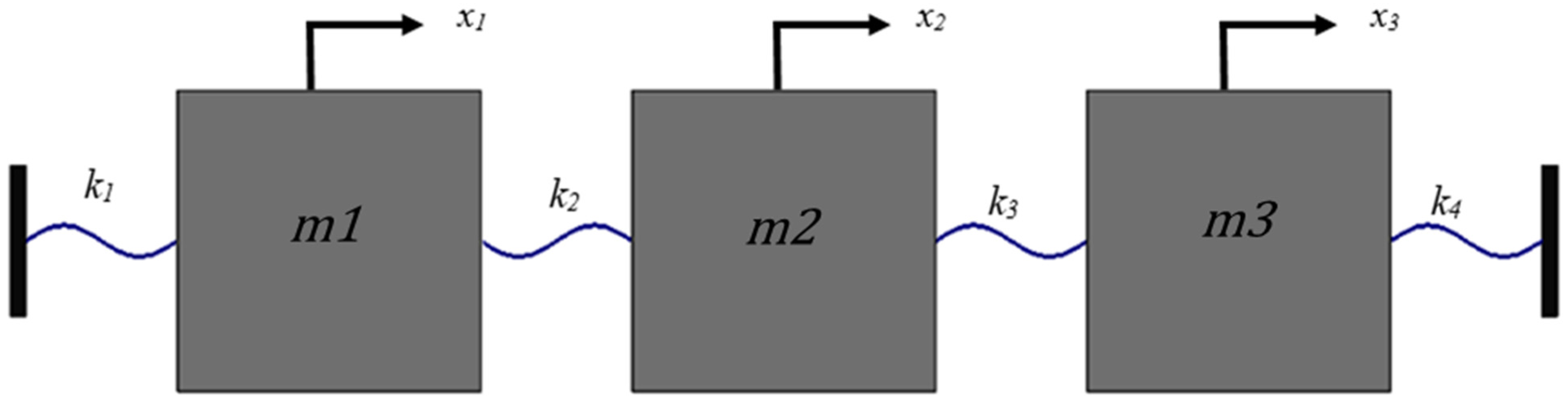
To demonstrate the working principle of RSO, we comprehensively analyze a three-degree-of-freedom (DOF) discrete mass system model with lumped parameters. We use two approaches: forward and reverse. The forward approach involves creating the model’s initial response, while the reversed approach is used to determine the model’s parameters based on response data. To simulate the model’s initial response, we create a forced response model in the ANSYS-22 R, Workbench harmonic analysis module with predetermined values for the spring stiffness. In the reversed approach, we consider the spring stiffness as an unknown parameter and calculate it by analyzing the model’s response, including the maximum amplitude response and resonant frequencies. To optimize the unknown parameters, we use the LHS technique and generate response surfaces using the genetic aggregation technique. The combination of LHS and genetic aggregation constructs an optimal Latin hypercube design, ensuring a more even and representative coverage of the entire design space compared to purely random sampling methods. Moreover, combining LHS and genetic aggregation techniques reduces the number of DOEs. The major advantages of using this technique are computational efficiency and metamodel accuracy, especially for high-dimensional problems such as propulsion shaft lines. Finally, we compare the optimized parameters to the initial assumed stiffness based on the least RMSE and PRESS, confirming the effectiveness of the RSO technique. Figure 1 illustrates the spring mass model used in the analysis.

The equation of the Motion for a system shown in Figure 1 can be written as,

$$\left[m\right]\left\{\ddot{x}\right\}+\left[k\right]\left\{x\right\}=\left\{F\right\}$$

(6)

where $\left[m\right]$ and $\left[k\right]$ are the mass and stiffness matrix, $\left\{F\right\}$ is the external excitation force vector. If the damping matrix $\left[C\right]$ is introduced in the model defined by Equation (6), then Equation (6) can be written as,

$$\left[m\right]\left\{\ddot{x}\right\}+\left[k\right]\left\{x\right\}+\left[C\right]\dot{\left\{x\right\}}=\left\{F\right\}$$

(7)

Equation (7) can be solved by using the FE based harmonic analysis tools utilizing the frequency domain approach [23,24] or by using the numerical technique. In this paper ANSYS modal and harmonic analysis module are used to generate the response data. The parameters used in the simulation are as follows.

$$m_1=1 \mathrm{k}\mathrm{g}, m_2=2 \mathrm{k}\mathrm{g}, m_3=1 \mathrm{k}\mathrm{g}, k_1=5.7\times {10}^5\frac{N}{m}, k_2=4.3\times {10}^5\frac{N}{m},$$

$$k_3=7.5\times {10}^5\frac{N}{m}, k_4=8.5\times {10}^5\frac{N}{m}$$

and modal damping ratios ${\zeta }_1={\zeta }_2={\zeta }_3=0.05$ are assumed for the simulation.

The resonant frequencies obtained from the Modal analysis are listed in

Table 1. Resonant frequencies of a three-DOFs system.

Mode No	Modal Frequency (Hz)
1	82.616
2	166.56
3	220.61

.

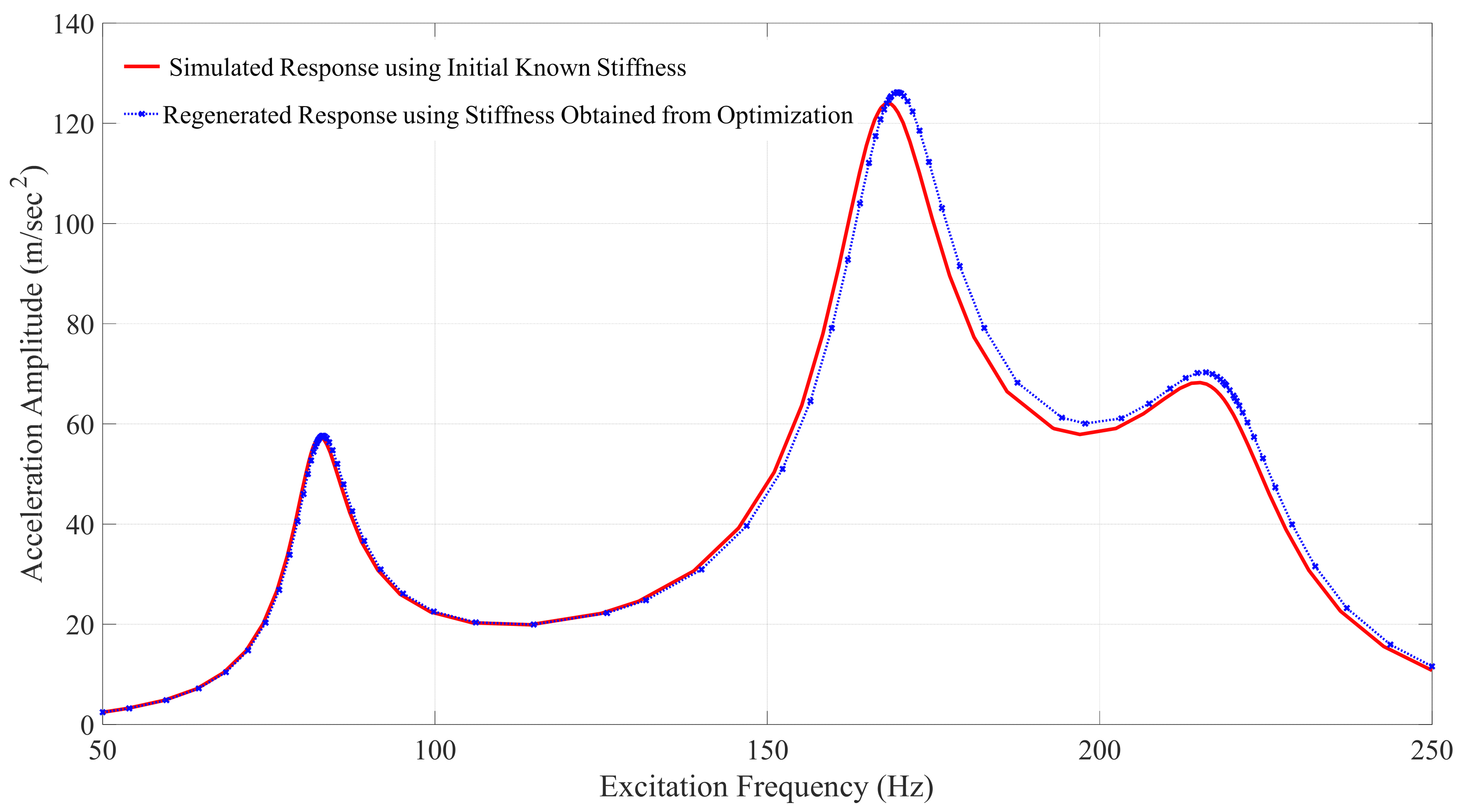
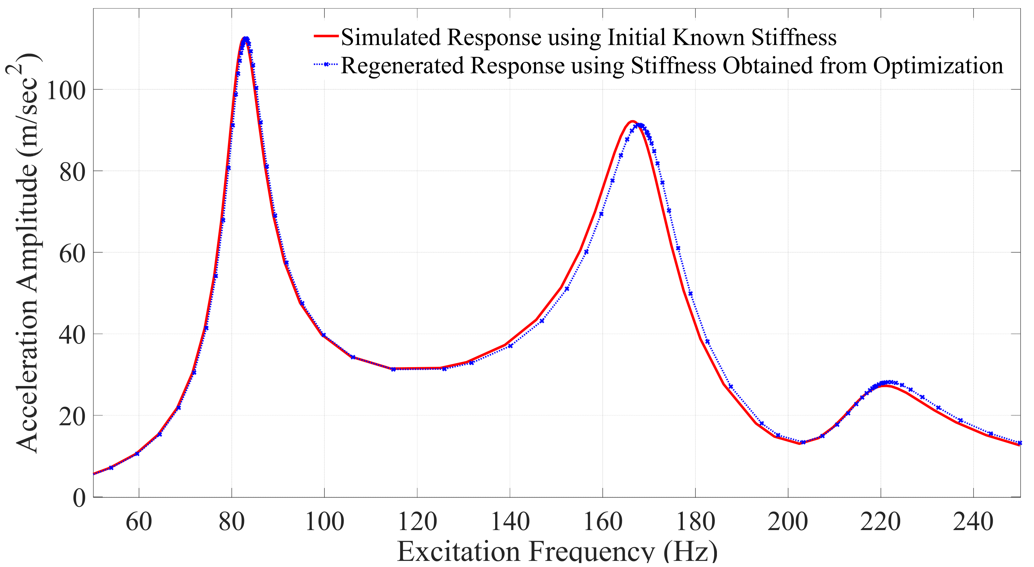
The harmonic analysis of a system shown in Figure 1 is carried out by exciting $m_3$ with a force of $50 \mathrm{N}$ harmonic at an excitation frequency range of (50–250) Hz (covering all three resonant frequencies), and the steady state amplitude at each frequency is recorded. The response of mass 2 at the excitation frequency range is shown in Figure 2 as a FRF. Having known one of the FRFs (Figure 2) and the resonant frequency shown in Table 1, the reverse approach for parameter estimation is carried out by assuming the four stiffnesses of the spring mass system to be unknown.

2.1.2. Reverse Approach for Parameter Identification

In the reverse analysis approach, the spring–mass system’s stiffness parameters are assumed to be unknown. The simulated response data from the forward approach shown in Figure 2 and the resonant frequencies presented in Table 1 are used as the output to obtain the unknown stiffness parameters by creating the response surfaces. The outputs utilized are the first mode, second mode, third mode resonant frequencies and the maximum acceleration responses at the corresponding resonant frequencies. The goal is to obtain the unknown stiffness parameters of the spring through the DOEs such that the difference between the measured output and the reconstructed output is minimal. For this, the design of experiment (DOE) is created using four spring stiffness parameters, which is the dependent variable, and the upper limit and lower limit of all the spring’s stiffness are assigned as $1\times {10}^5 \mathrm{t}\mathrm{o} 9.5\times {10}^5 \mathrm{N}/\mathrm{m}$. To establish the correlation between the stiffness of each of the four springs and the desired output, 25 design points are generated to create the response surfaces. After the optimization, three candidate models are obtained; they are then cross verified using the PRESS. The candidate model with the lowest value of PRESS is taken as the best model. The associated stiffness parameters of the best model and the comparison with the original spring stiffness is tabulated in

Table 2. Comparison of original and optimized stiffness parameters.

Parameters	Original Stiffness (N/m)	Optimized Stiffness (N/m)	% Error
$k_1$	$5.7\times {10}^5$	$5.786\times {10}^5$	1.4
$k_2$	$4.3\times {10}^5$	$4.39\times {10}^5$	2.09
$k_3$	$7.5\times {10}^5$	$7.5887\times {10}^5$	1
$k_4$	$8.5\times {10}^5$	$8.510\times {10}^5$	0.11

. As shown in Table 2, the error between the original stiffness and the optimized stiffness is less than 2%, indicating the robustness of the implemented optimization technique. Figure 3, Figure 4 and Figure 5 show the comparison of the harmonic response of the model from the forward approach and the reversed approach. It should be noted that only mass 2 response data and three resonant frequencies are taken for optimization. The results will be identical if mass 1 or mass 3 response data are taken for analysis. 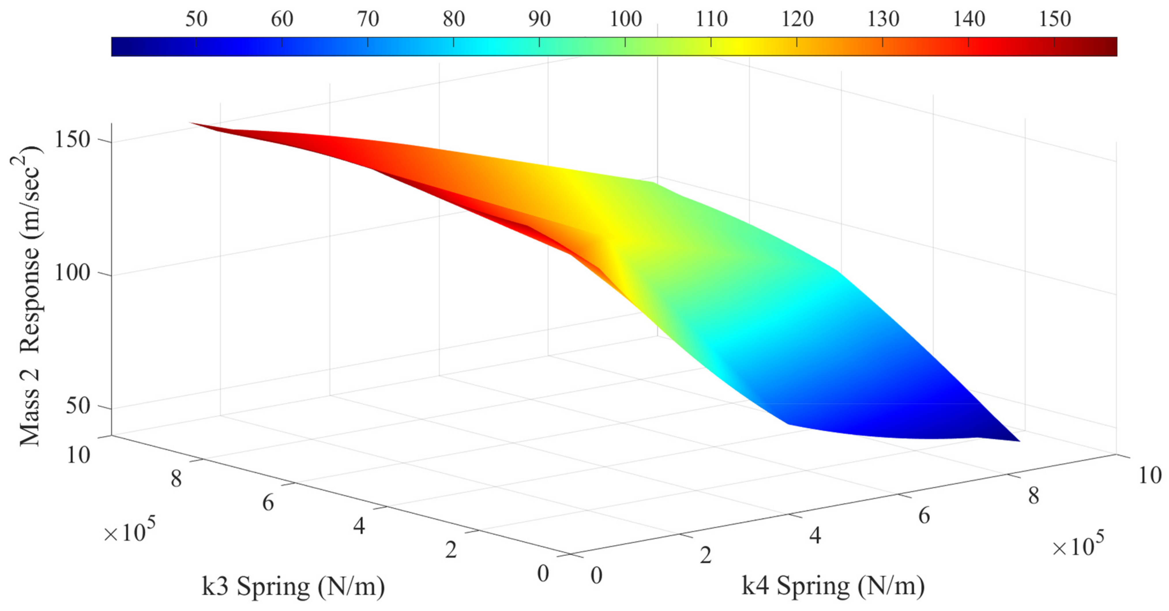Similarly, Figure 6 and Figure 7 show the response plot between the dependent variable and the objective function. While the spring stiffness variation is taken from $1\times {10}^5$ to $9\times {10}^5 \mathrm{N}/\mathrm{m}$ during DOE, the wide range of variation can be taken even starting from 100 to $1\times {10}^9 \mathrm{N}/\mathrm{m}$; the only difference will be the computational cost; one needs to create a huge number of design points, resulting in a longer time for convergence. Furthermore, the system can be excited with forces in all masses to generate excitation data, and the excitation amplitude can be selected to any value. However, this may lead to longer computational time. It is important to note that the system should be designed to operate within a linear region, and large deformation theory should not be used while modeling it. If the large deformation theory is used, the system will not behave linearly. As a result, applying the algorithm becomes cumbersome due to the deviation of FRFs from the linearity.

3. Experimental Analysis of Propulsion Shaft System

An experimental setup was designed to demonstrate the system identification concept using the RSO algorithm. The proposed experimental model was fabricated in-house by downscaling the suitable available model in the existing literature [17]. Figure 7 shows the test model of the propulsion system used for longitudinal excitation testing. The details of the experimental setup consist of the propeller, intermediate shafts, thrust bearing, radial contact ball bearings, different types of couplings, and the variable frequency drive motor. The variable frequency drive motor was utilized during the experiment to support the shaft. The structure’s right side has an intermediate shaft connected to the motor by a jaw coupler and then a thrust bearing and the first intermediate bearing follow it. Then, a rigid coupler connects the first intermediate shaft to the second one. Finally, a propeller is attached to the end of the second intermediate shaft using set screws. The material properties and the detailed dimensions of the individual parts are listed in

Table 3. Details of the components used in the assembly.

S/N	Components	Materials	Dimensions	Nomenclature
1	Intermediate shaft 1 (rotary shaft)	440 C stainless steel	500 mm × 10 mm (length × radius)
2	Intermediate shaft 2 (rotary shaft)	440 C stainless steel	500 mm × 10 mm (length × radius)	ID: Inner Diameter OD: Outer Diameter
3	Thrust ball bearing	Stainless steel	ID: 20 mm; OD: 37 mm Thickness: 12 mm
4	Set screw shaft coupling	303 stainless steel	ID: 20 mm Length: 50 mm
5	Mounted ball bearing	Cast iron housing Stainless steel	ID: 20 mm Width: 34 mm
6	Propeller (left hand)	Stainless steel	¾ in shaft diameter 3½ in pitch
7	Jaw coupling hub	Sintered iron	ID: 20 mm (shaft) ID: 5/8 in (motor)

. To carry out forced vibration tests, we utilized a modal exciter from PCB Piezotronics. This exciter has a peak sine force of 58 N (13 lbf) and a peak-peak stroke of 18 mm (0.7″). It also features an adjustable collet stinger attachment and a through-hole armature design, as shown in Figure 7. We attached an ICP impedance head to the exciter for the measurement of the input acceleration/force excitation signal. Experiments were conducted in two arrangements: (i) lateral or transverse excitation, and (ii) longitudinal or axial excitation.

3.1. Transverse (Lateral) Vibration Excitation

Lateral vibration in the propulsion shaft system occurs due to misalignment of the shaft and manufacturing defects in the gearing system. In order to mimic the lateral vibration in the laboratory environment, an experimental setup was designed by using an exciter that directly excites the shaft in the transverse direction. Figure 8 shows our experimental design for the transverse vibration setup, where the intermediate shaft was excited using the modal shaker, resulting in the lateral vibration of the entire assembly. Two PCB (352C22) accelerometers were used to record the transverse vibration of the shaft: one behind the propeller and the other exactly at the intermediate shaft face, as shown in Figure 8.

During the experiment, we utilized harmonic excitation within the frequency range of 50–1000 Hz, incorporating a 1 Hz sweep sine input and an acceleration excitation amplitude of 0.1 g, implementing an open loop controller. The steady state response of two accelerometers was recorded at each excitation frequency using the Crystal Instruments EDM (Engineering Data Management) 10.0 software. To identify the vibration mode of the assembly, we plotted the response of the shaft system within the given excitation frequency range using the steady state response of the shaft at each excitation frequency. Figure 9 displays the lateral response of the shaft located near the propeller and away from the propeller. As anticipated, the response of the shaft close to the propeller was greater than that of the shaft located away from the propeller, as there was no support system in place near the propeller.

3.2. Longitudinal Vibration Excitation

For the longitudinal experimental setup, the propeller end was excited with very low excitation with an amplitude of 0.1 g to imitate the real-world excitation scenario provided by the unsymmetrical stern flow near the propeller due to the current in the water. Two accelerometers were attached near the propeller hub face, and another one was attached to the face of the rigid coupling, 450 mm away from the propeller. The purpose of this setup was to analyze the structural characteristics in the vicinity of the propeller and to observe any changes in vibration response along the shaft. Figure 10 shows the vibration response of the shaft near and away from the propeller at an excitation acceleration of 0.1 g. Since the shaft is short as compared to the practical application, it is expected that the longitudinal mode of the vibration of shaft is high as compared to the practical scenario, which is evident from Figure 11.

4. Finite Element Modeling of Propulsion Shaft System

The FEM of the propulsion shaft system is carried out in the ANSYS Release 23 Workbench environment. The goal is to define the suitable boundary conditions and connections in the assembly while creating the finite element model such that the structure’s dynamic behavior is as similar as possible between the actual tested model response and the numerically simulated response. The detailed 3D model of the propulsion shaft system is modeled using SolidWorks and is imported to the ANSYS Workbench environment. The imported simplified model for FEM analysis is shown in Figure 11. As illustrated in Figure 11, the model consists of two ball bearing housing that connect with the shaft using four springs each, and the thrust bearing is suppressed where four additional springs are added as a body-to-ground connection in a shaft. The boundary conditions imposed are three fixed supports: one on the end of the shaft, which connects to the motor; the other two fixed supports are used on the faces of the bearing housing where the screws are used to fix it to the support as shown in the experimental model in Figure 7 and Figure 8, respectively.

4.1. Selection of Bearing Stiffness Parameters and Updating the Parameters by Using Response Surface Optimization

The FEM model updating process starts by choosing a suitable set of numerical model parameters (unknown bearings stiffness) that are efficiently changed during the process. These parameters represent unknown properties in the experiment. The fewer unknown parameters, the more efficient the FEM. If the number of unknown parameters exceeds the output parameters, the optimization may produce irrelevant and ill-conditioned results. Some unknown parameters in a system have a more significant impact on a structure’s properties than others. Parameter correlation looks at how sensitive each input parameter is to the output parameter, which is essential in optimizing a model. Parameters with low correlation can be given less priority or ignored to reduce the computational time needed during optimization. The model that we consider consists of 12 springs. The first four springs represent the modeled thrust ball bearing, and the connection type used is the body to ground. The other eight spring connections are connected from body to body from the shaft to the bearing housing (two ball bearings). This is done to represent the contact between the inner ring of the bearing and the shaft as well as to create a parameter for the parametric study to find the unknown longitudinal (ANSYS uses the term Longitudinal stiffness for all the radial stiffness) stiffness, which is then used as DOEs to create a response surface and then lead to optimization. These 12 longitudinal stiffnesses are used as input parameters and provided with lower and upper bounds, where the lower bound is set to ${10}^5$ N/m and the upper bound is set to ${10}^9$ N/m. A total of three output parameters are chosen: the shaft’s first mode resonant frequency, the second mode resonant frequency, and its maximum amplitude response obtained from the transverse vibration test. Since only three output parameters are utilized to update the structural model, and there are 12 unknown stiffnesss, the problem is ill-conditioned. It is well known that not all the bearing stiffnesses in four directions [9,17] for each bearing will contribute to the transverse vibration in the excitation frequency range (50–1000 Hz) of interest; for this, a design of experiment is carried out in the ANSYS optimization module. The fundamental procedure in the design of experiment consists of determining projected values of the response features at various design points (DPs) in the parameter space by simulating each DP. This response surface will be a placeholder for the FE simulation model (Figure 12). The number of DPs created depends upon the response surface method to be established. The DOE of test sample points is used to fit the response surface, which is the point in response surface technique. A good selection of sample points can reduce the calculation cost of DOE and improve the accuracy of the response surface. The commonly used point selection method at this stage is to fill the design space with the most effective and minimum sample points as much as possible. The positions of the test sample points meet certain symmetry and uniformity requirements. We utilize the Latin hypercube sampling method with full quadratic sample methods to create the design points through which the response surface is generated. Once the response surface is generated, local sensitivity analysis is conducted to see how each input parameter (bearing stiffness) affects the output response. This information helps to eliminate parameters that do not correlate with the output. Figure 13 shows the sensitivity analysis of the 12 stiffness parameters, of which only three stiffness parameters are sensitive by more than 20%. So, an ill-conditioned problem is synthesized into a well-posed problem by optimizing those three spring parameters.

After synthesizing the problem into a well-posed one, the optimization process involves defining objectives and constraints for the output parameters. The target value is selected from the experimental measurements obtained, as shown in Figure 9. To carry out the optimization, the multi-objective genetic algorithm (MOGA) method is used, which is a variant of the popular non-dominated sorted genetic algorithm-II (NSGA-II) based on controlled elitism concepts. This method supports multiple objectives and constraints and aims to find the global optimum. Figure 14 displays the response of the optimized model and the experimental model. The error between the two models is less than 10% in terms of the resonant frequency, and the maximum amplitude of vibration, which is considered an acceptable range for a complex problem with several unknown variables, and the accuracy of the results is close to those available in the existing literature [23,24]. It is worth noting that only three stiffness parameters of the bearing contributed to the transverse vibration problems in the chosen excitation frequency range. The other stiffness parameters may contribute to the longitudinal excitation or other higher modes that are not excited.

4.2. Limitations of the Study

The study is carried out by designing an experimental setup to generate the dynamic response of the propulsion shaft utilizing different types of bearings and couplers. The physical model was scaled to smaller dimensions so that it could be set up and tested in the laboratory environment. The marine shaft in the actual environment is extremely long, so the longitudinal resonant frequencies are usually below 200 Hz. In our research problem, since the shaft size is small compared to the practical applications, the resonant frequencies are higher than 200 Hz. Nevertheless, the algorithm implemented does not affect resonant frequency variation and has the same accuracy if all the resonant frequencies are below 200 Hz. The only thing one should consider while performing vibrations suppression study in marine shafts is to develop a similitude model with the same longitudinal resonant frequency compared to the actual practical applications.

5. Conclusions

This paper presents the detailed dynamic analysis and system identification technique of a marine propulsion shaft system subjected to dynamic excitation. The detailed dynamic analysis in a propulsion shaft system is conducted by designing a laboratory-based suitable scaled experimental setup that can induce significant vibration when subjected to dynamic excitations. The shaft is excited in the lateral and the longitudinal direction by using the PCB modal shaker in the excitation frequency range of (50–1000) Hz. The steady-state response of the system at each excitation frequency is recorded by using PCB accelerometer data utilizing the Crystal Instruments Engineering Data Management (EDM) 10.0 software. Frequency response functions are created at the measured degree of freedom by utilizing the steady-state data, and the spectrum of the response over the excitation frequency band is created. The system identification technique is carried out using the response surface optimization technique. First, a numerical example is presented to demonstrate the concept of response surface optimization using the three-DoF lumped parameter model. Similar to the experimental approach, the response spectrum of the three-DoF model is created through FE modeling utilizing the ANSYS R-22 software. Once the response spectrum is calculated, the response surface optimization is used to estimate the spring stiffness, which is then compared with the original stiffness values to demonstrate the efficacy of the proposed algorithm. Following the numerical example, the same algorithm (response surface optimization) is utilized to update the FE model in a propulsion shaft system using the experimental data measured through harmonic excitation. The results show that the ill-conditioned problem can be resolved to a well-posed problem by performing the sensitivity analysis, and the unknown parameters of the structure can be estimated by using the design of experiment techniques in the FE-based environment. The efficiency of this approach lies in its ability to resolve complex problems and generate valuable insights that can drive innovation and progress. Based on the optimized model, the future research area of this project is to develop a suitable methodology to suppress the vibrations in the propulsion shaft line. The work includes (i) the development of passive vibration control algorithms utilizing the elastomeric coating to reduce the transverse and longitudinal vibrations, (ii) the development of a hyperelastic dynamic model for elastomeric materials, and (iii) an analysis of the vibration suppression capacity of the elastomeric material in the propulsion shaft lines.

References

1. Cui, W.; Fu, S.; Hu, Z. (Eds.) Encyclopedia of Ocean Engineering; Springer Nature: Singapore, 2022. [Google Scholar]
2. Xie, X.; Ren, M.; Zhu, Y.; Zhang, Z. Simulation and experiment on lateral vibration transmission control of a shafting system with active stern support. Int. J. Mech. Sci. 2020, 170, 105363. [Google Scholar] [CrossRef]
3. Huang, Q.; Liu, H.; Cao, J. Investigation of lumped-mass method on coupled torsional-longitudinal vibrations for a marine propulsion shaft with impact factors. J. Mar. Sci. Eng. 2019, 7, 95. [Google Scholar] [CrossRef]
4. Jia, X.J.; Fan, S.D. Analysis of the flexural vibration of ship’s tail shaft by transfer matrix method. J. Mar. Sci. Appl. 2008, 7, 179–183. [Google Scholar] [CrossRef]
5. Chahr-Eddine, K.; Yassine, A. Forced axial and torsional vibrations of a shaft line using the transfer matrix method related to solution coefficients. J. Mar. Sci. Appl. 2014, 13, 200–205. [Google Scholar] [CrossRef]
6. Li, C.; Huang, X.; Hua, H. Dynamic modeling and analysis of axial vibration of a coupled propeller and shaft system. J. Mech. Sci. Technol. 2016, 30, 2953–2960. [Google Scholar] [CrossRef]
7. Chu, W.; Zhao, Y.; Zhang, G.; Yuan, H. Longitudinal Vibration of Marine Propulsion Shafting: Experiments and Analysis. J. Mar. Sci. Eng. 2022, 10, 1173. [Google Scholar] [CrossRef]
8. Zhang, G.; Zhao, Y.; Li, T.; Zhu, X. Propeller excitation of longitudinal vibration characteristics of marine propulsion shafting system. Shock Vib. 2014, 2014, 413592. [Google Scholar] [CrossRef]
9. Huang, Q.; Zhang, C.; Jin, Y.; Yuan, C.; Yan, X. Vibration analysis of marine propulsion shafting by the coupled finite element method. J. Vibroeng. 2015, 17, 3392–3403. [Google Scholar]
10. Yucel, A.; Arpaci, A. Free and forced vibration analyses of ship structures using the finite element method. J. Mar. Sci. Technol. 2013, 18, 324–338. [Google Scholar] [CrossRef]
11. Firouzi, J.; Ghassemi, H.; Shadmani, M. Analytical model for coupled torsional-longitudinal vibrations of marine propeller shafting system considering blade characteristics. Appl. Math. Model. 2021, 94, 737–756. [Google Scholar] [CrossRef]
12. Tchomeni, B.X.; Alugongo, A. Modelling and dynamic analysis of an unbalanced and cracked cardan shaft for vehicle propeller shaft systems. Appl. Sci. 2021, 11, 8132. [Google Scholar] [CrossRef]
13. Chen, F.; Chen, Y.; Hua, H. Coupled vibration characteristics of a submarine propeller-shaft-hull system at low frequency. J. Low Freq. Noise Vib. Act. Control. 2020, 39, 258–279. [Google Scholar] [CrossRef]
14. Feng, F.Z.; Kim, Y.H.; Yang, B.S. Applications of hybrid optimization techniques for model updating of rotor shafts. Struct. Multidiscip. Optim. 2006, 32, 65–75. [Google Scholar] [CrossRef]
15. Kwon, K.S.; Lin, R.M. Frequency selection method for FRF-based model updating. J. Sound Vib. 2004, 278, 285–306. [Google Scholar] [CrossRef]
16. Tiwari, R.; Lees, A.W.; Friswell, M.I. Identification of dynamic bearing parameters: A review. Shock Vib. Dig. 2004, 36, 99–124. [Google Scholar] [CrossRef]
17. Jalali, H.; Ahmadian, H. Model identification and dynamic analysis of ship propulsion shaft lines. J. Theor. Appl. Vib. Acoust. 2015, 1, 85–95. [Google Scholar]
18. Xu, F.; Li, C.R.; Jiang, T.M.; Zhang, D.P. Fatigue life prediction for PBGA under random vibration using updated finite element models. Exp. Tech. 2016, 40, 1421–1435. [Google Scholar] [CrossRef]
19. Wan, Y.; Huang, H.; Pecht, M. Thermal fatigue reliability analysis and structural optimization based on a robust method for microelectronics FBGA packages. IEEE Trans. Device Mater. Reliab. 2015, 15, 206–213. [Google Scholar] [CrossRef]
20. Lee, J.; Jeong, H.; Jang, G. Optimization of the Boundary Conditions of a Board Level Reliability Test Board to Maximize the Fatigue Life of Ball Grid Array Solder Joints under Thermal Cycling and Random Vibration. Materials 2024, 17, 755. [Google Scholar] [CrossRef]
21. Doranga, S.; Wu, C.Q. Parameter identification for nonlinear dynamic systems via multilinear least square estimation. In Special Topics in Structural Dynamics, Volume 6: Proceedings of the 32nd IMAC, A Conference and Exposition on Structural Dynamics; Springer International Publishing: Berlin/Heidelberg, Germany, 2014; pp. 169–182. [Google Scholar]
22. Gharaibeh, M. Identification of printed circuit boards mechanical properties using response surface methods. Microelectron. Int. 2022, 39, 38–47. [Google Scholar] [CrossRef]
23. Doranga, S.; Wu, C. Study of nonlinear effects in a bolted joint using the base excitation as an input. J. Vibroeng. 2021, 23, 1109–1128. [Google Scholar] [CrossRef]
24. Doranga, S.; Zhou, J.; Poudel, R. Influence of Printed Circuit Board Dynamics on the Fretting Wear of Electronic Connectors: A Dynamic Analysis Approach. J. Electron. Test. 2022, 38, 493–510. [Google Scholar] [CrossRef]
Figure 1. A three-DOFs spring mass model.
Applmech 05 00018 g001
Figure 2. FRF of mass 2 due to excitation at mass 3.
Applmech 05 00018 g002
Figure 3. FRF of mass 1 due to excitation at mass 3.
Applmech 05 00018 g003
Figure 4. Simulated and Regenerated FRF Response of mass 2 due to excitation at mass 3.
Applmech 05 00018 g004
Figure 5. FRF of mass 3 due to excitation at mass 3.
Applmech 05 00018 g005
Figure 6. Response surface plot between spring stiffness and second mode response of mass 2.
Applmech 05 00018 g006
Figure 7. Longitudinal excitation test setup.
Applmech 05 00018 g007
Figure 8. Lateral excitation test setup.
Applmech 05 00018 g008
Figure 9. Steady state response of the shaft due to lateral excitation.
Applmech 05 00018 g009
Figure 10. Steady state response of the shaft due to longitudinal excitation.
Applmech 05 00018 g010
Figure 11. Model of the Propulsion Shaft System for FEM Analysis in ANSYS Workbench.
Applmech 05 00018 g011
Figure 12. Response surface plot of back ball bearing, thrust bearing and maximum second mode response.
Applmech 05 00018 g012
Figure 13. Local sensitivity analysis of bearing stiffness.
Applmech 05 00018 g013
Figure 14. Comparison of FEM and experimental results of the transverse vibration of the propulsion shaft after response surface optimization.
Applmech 05 00018 g014