Signal and Image Processing in Biomedical Photoacoustic Imaging: A Review

Abstract

Photoacoustic imaging (PAI) is a powerful imaging modality that relies on the PA effect. PAI works on the principle of electromagnetic energy absorption by the exogenous contrast agents and/or endogenous molecules present in the biological tissue, consequently generating ultrasound waves. PAI combines a high optical contrast with a high acoustic spatiotemporal resolution, allowing the non-invasive visualization of absorbers in deep structures. However, due to the optical diffusion and ultrasound attenuation in heterogeneous turbid biological tissue, the quality of the PA images deteriorates. Therefore, signal and image-processing techniques are imperative in PAI to provide high-quality images with detailed structural and functional information in deep tissues. Here, we review various signal and image processing techniques that have been developed/implemented in PAI. Our goal is to highlight the importance of image computing in photoacoustic imaging.

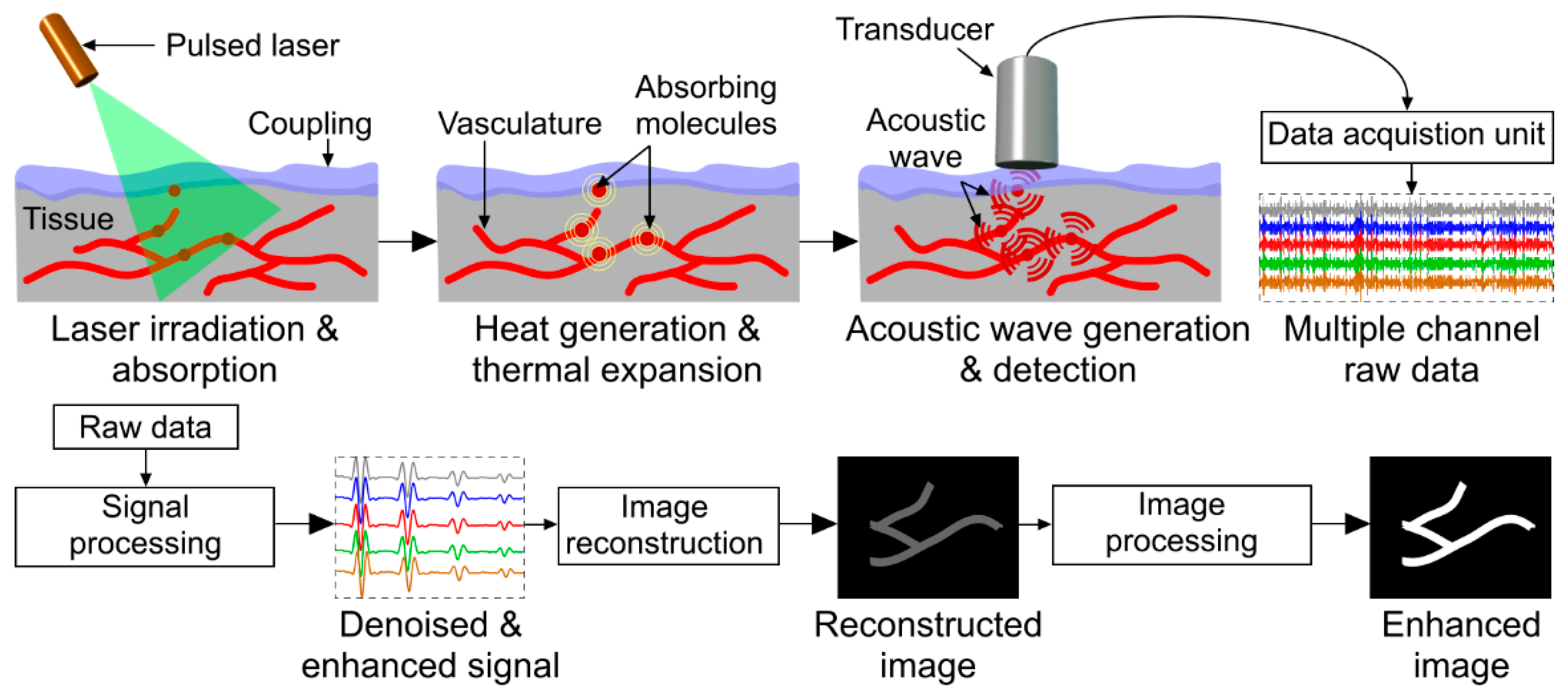
1. Introduction

Photoacoustic imaging (PAI) is a non-ionizing and non-invasive hybrid imaging modality that has made significant progress in recent years, up to a point where clinical studies are becoming a real possibility [1,2,3,4,5,6]. Due to the hybrid nature of PAI, i.e., optical excitation and acoustic detection, this modality benefits from both rich and versatile optical contrast and high (diffraction-limited) spatial resolution associated with low-scattering nature of ultrasonic wave propagation [7,8,9,10,11]. Photoacoustic imaging breaks through the diffusion limit of high-resolution optical imaging (~1 mm) by using electromagnetic energy induced ultrasonic waves as a carrier to obtain optical absorption information of tissue [12,13]. PAI, being a relatively new imaging modality, can effectively realize the structural and functional information of the biological tissue, providing a powerful imaging tool for studying the morphological structure, physiological, pathological characteristics, and metabolic functions in biological tissues [14,15,16].

The PA effect initiates when optically absorbing targets (absorbers/chromophores) within the tissue are irradiated by a short (~nanosecond) pulse laser [17]. The pulse energy is absorbed by the target and converted into heat, generating a local transient temperature rise, followed by a local acoustic pressure rise through thermo-elastic expansion [18,19,20,21].

The pressure waves propagating as ultrasonic waves, are detected by ultrasonic transducers present outside the tissue, termed as raw data (Figure 1). These data carry information of inherent acoustic and optical properties (as presented in [22]) of the absorbers in combination with noisy data originating from electromagnetic interferences. The acquired data are further processed (known as signal processing) to extract the desired PA signal from the noisy background and utilized to reconstruct a PA image [23,24]. These images represent internal structures and corresponding functionality of the tissue target region [25,26,27,28,29,30,31]. Several image reconstruction algorithms have been studied for PA imaging [30,32,33,34] where the reconstruction algorithms can be interpreted as an acoustic inverse source problem [35]. Conventional PA image reconstruction algorithms assume that the object of interest possesses homogeneous acoustic properties [36]. However, the tissue medium in reality is heterogeneous with spatially variant sound of speed and density distribution [37]. This introduces varying effects known as acoustic aberration (i.e., amplitude attenuation, signal broadening, mode conversion) that eventually amplifies the low frequency signals and affects the small wavelengths, corresponding to the microstructures and sharp edges. Consequently, image resolution; one of the main contributions of PAI, is forsaken. Moreover, due to variable acoustic aberration, significant distortions and artifacts are also introduced [38,39,40]. There have been advancements of PA image reconstruction algorithms that can compensate for variations in the acoustical properties [41,42,43,44,45,46], however, further image enhancement in terms of post-processing is essential.

To accurately obtain the morphological and functional information of the tissue chromophores, the initial goal is to retrieve the initial pressure distribution inside the object due to the absorbed laser energy [47]. Therefore, knowledge of the local optical fluence (optical energy per unit area) in biological tissue is of fundamental importance for biomedical PA imaging [48]. However, initial pressure distribution is a function of depth (lateral and axial), wavelength, thermal properties (i.e., specific heat, Gruneisen parameter) and optical properties (i.e., absorption and scattering coefficient, anisotropy factor, and refractive index) of the medium including the tissue target. To simplify the initial pressure distribution retrieval process, the amount of optical fluence reaching the region-of-interest (ROI) necessitates to consider homogenous distribution of light [49]. However, in reality, the strong optical absorption by heterogeneous turbid superficial tissue structure pose major obstruction in irradiating the actual target located deep inside the tissue medium with sufficient optical energy [7,10,16]. This limits accurate quantification measurement such as oxygen saturation, blood volume calculations etc. [50]. There are several methods [36,51] have been proposed to optimize the fluence decay, however, these models are based on optical properties of different tissue types available in literature. Unfortunately, the exact optical properties of biological tissues are unknown, the medium is not homogeneous, which limits the practicality of these methods [48]. Moreover, optical fluence incident upon the tissue must be limited within the pre-defined safety limit. In addition, the scattering characteristics of the tissue alters the generated PA signal [10]. Therefore, the amplitude of a raw PA signal generated from a deep tissue structure is very low. This limited penetration depth and optical contrast also leads to the aliasing effect. Typically, detected PA signals of ideal optical absorbing particle are of bipolar N-shape [52,53,54] however, the PA signals produced within a complicated biological tissue can be the combination of individual N-shape pulses from adjacent microstructures. Consequently, the PA signals from small targets are deteriorated and even buried by the bipolar signal originating from a nearby relatively large target. These phenomena lead to aliasing and distortion in the final image [52]. In addition to the aliasing effect, the efficacy of the conversion from optical absorption to acoustic wave generation is often affected by the presence of high background noise [55,56]. The PA signals are often corrupted by background noise, from the medium and the transducer, respectively [18]. White Gaussian noise is one of the most common models for these types of randomly distributed thermal and electronic noise [57]. Furthermore, fixed-pattern noise caused by electromagnetic interference is another major source of background noise. The combination of these different types of noises offsets the PA signal, leading to a low signal-to-noise ratio (SNR), consequently producing low quality images [58,59,60,61].

Therefore, several studies have attempted to develop signal enhancement and image post-processing algorithms to either extract the original, attenuated PA signal or to improve the existing one by various filtering techniques. [58,62,63]. In many cases, these approaches were incorporated into the image reconstruction algorithms to achieve noise- and artifact-free PA images [64,65,66,67,68,69,70]. To further improve the prevalent image processing technique, different deep learning architectures have also been proposed [71,72].

The objective of this review article is to categorically discuss the attributes of various signal and image processing techniques used in PA. The review process is categorized into three aspects of improving PA images: (i) PA signal pre-processing prior to image reconstruction and (ii) image post processing after the image reconstruction, and (iii) deep learning techniques. The search protocol used for this review study is as follows. For the first aspect, a PubMed database search of “photoacoustic” AND “signal processing” yielded 141 results with 61 published in the last five years. For the second aspect: “photoacoustic” AND “image enhancement” yielded 207 results with only 55 published in the last five years. Finally, the third aspect: photoacoustic” AND “image processing” yielded 198 articles published in the last 5 years. Among these articles 10 are associated with “image segmentation”, 10 articles are relevant to “image classification”. Here, we have considered only the publications where the processing concept and development methods are clearly demonstrated with appropriate experimental evaluations. To date, several major review articles have been published regarding the photoacoustic imaging and most are based on instrumentation and configurations. However, according to the authors’ best knowledge, there is no dedicated review article that summarizes the key aspects of the signal and image processing in photoacoustic imaging.

Initially, we explored the root causes of diminished PA signal and corresponding degraded image quality. This follows with exploring the merit and demerits of various approaches to improve the photoacoustic signal and image quality as pre- and post-processing techniques respectively. Finally, we explore the articles where different deep learning based image processing algorithms have been utilized for improving diagnostic purposes such as classification and segmentation.

2. Photoacoustic (PA) Signal Pre-Processing Techniques

The complex biological tissue structures consist of several overlaying chromophores with different absorption coefficients. The PA signal from a less absorbing chromophore is either lost or overshadowed by a nearby comparatively higher absorbing chromophores. Moreover, the incident laser energy limitation imposed by ANSI (American National Standards Institute) and the optical path being highly attenuated due to the scattering in the tissue [73], results in generating a low amplitude PA signal by poorly illuminated deeper structures within the tissue. This results in the PA signal being camouflaged within the background noise upon reception by the transducer, leading to a reconstruction of a very low SNR images [18]. Specifically, when a low-cost PA system based on low power light-emitting diodes (LEDs) are utilized, the PA signals generated from imaging target are strongly submerged in the background noise signal [37]. A typical PA signal is usually contaminated with background noises (i.e., combination of electronic and system thermal noise [56,58]. These noises are generally originated from external hardware (i.e., transducer elements, acquisition system, and laser sources). Usually, the noise from the laser source dominates at the kilohertz frequency range and attenuates following an inverse function of frequency (1/f) [74,75]. At the megahertz frequency range, the noise from the laser source becomes less dominant [76]. Instead, the signal amplifier, the photodetector, and the data acquisition card become the major noise sources. On the other hand, biological tissue being a highly scattering medium introduce major attenuating events for the generated PA signal before it propagates and is received by transducers [73]. Several pre-processing techniques to improve the PA signal to noise ratio upon reception by transducers are reviewed in the following subsections.

2.1. Averaging

Signal averaging is perhaps the easiest and most common way of improving the signal quality by getting rid of uncorrelated random noise [77]. For signal averaging two schemes can be employed: (1) the raw pressure signals can be averaged coherently prior to signal processing; or (2) each of the received chirps is processed independently and the resulting correlation amplitudes are averaged [78]. These two methods define the logistics of data acquisition and may influence design of the system hardware and software for efficient signal processing. The former technique demands strict phase consistency of multiple excitation chirps and accumulation of multiple waveforms, while the latter allows for rapid processing of incoming chirps and summation of the final products to reduce noise [79]. However, the latter technique does not consider the phases of individual chirps and constitutes incoherent averaging during post-processing. Averaging specifically improves the SNR of the PA signals, particularly if the PA signal components being averaged are correlated as shown in Figure 2. A distinctive improvement by averaging method necessitates the acquisition of large number of PA signals from the same location. This acquisition number typically ranges from few hundreds to several thousands which makes this technique extremely time consuming, computationally exhaustive, and ineffective for moving targets [54].

2.2. Signal-Filtering Techniques

Signal-filtering techniques are often more effective when used with Fourier transformation methods. It involves selective component discarding of specific frequency bands. However, losing components of the actual PA signal along with the noise in those frequency ranges is inevitable [60]. To avoid this scenario, in [59], an adaptive and fast-filtering method to denoise and enhance the PA signal was presented. However, unlike a conventional adaptive noise canceller, this method does not require a prior knowledge of the characteristics of the signal. In fact, the reference signal was basically a time shifted version of the primary input signal. Due to using a reduced number of epochs in averaging, this algorithm created a smaller PA peak time-shift and signal-broadening. A PA microscopy image with the size of 200 × 200 pixels using the proposed method took about 1 s, allowing near real-time PA microscopy. Najafzadeh et al. [64] proposed a signal denoising method based on a combination of low-pass filtering and sparse coding (LPFSC). In the LPFSC method, the PA signal can be modeled as the sum of low frequency and sparse components, which allows for the reduction of noise levels using a hybrid alternating direction method of multipliers in an optimization process. Fourier and Wiener deconvolution filtering are two other common methods used for PA signal denoising prior to back projection algorithm [80,81,82]. Typically, a window function is used to limit the signals within a specific bandwidth and leads the high-frequency components to zero [83] followed by a convolution between PA signals and illumination pulse and/or ultrasound transducer impulse response. A Wiener filter is specifically utilized to remove the additive noise. Sompel et al. [84] compared the merits of a standard Fourier division technique, the Wiener deconvolution filter, and a Tikhonov L-2 norm regularized matrix inversion method. All the filters were used with the optimal setting. It was found that the Tikhonov filter were superior as compared to the Wiener and Fourier filters, in terms of the balance between low and high frequency components, image resolution, contrast to noise ratio (CNR), and robustness to noise. The results were evaluated through imaging in vivo subcutaneous mouse tumor model and a perfused and excised mouse brain as shown in Figure 3A. Moradi et al. [85] proposed a deconvolution-based PA reconstruction with sparsity regularization (DPARS) technique. The DPARS algorithm is a semi-analytical reconstruction approach where the directivity effect of the transducer is taken into account. The distribution of absorbers is computed using a sparse representation of absorber coefficients obtained from the discrete cosine transform.

2.3. Transformational Techniques

Wavelet transform based filtering techniques have become an effective denoising method. This frequency-based transform decomposes the signals into a series of basis functions with different coefficients. Usually the smaller coefficients corresponds to the noisy signals, that can be removed using thresholding [88]. In discrete wavelet transform denoising, firstly a suitable mother wavelet is selected and then decomposition, thresholding and reconstruction steps are performed. Mother wavelet selection is the most critical step and depends on the wavelet characteristics or the similarity between the signal and mother wavelet [89]. The decomposition step is carried out by selecting the appropriate degree of decomposition [90]. In decomposition steps, low-pass and high-pass filters are used based on the characteristics of the mother wavelet. The output of these filters, respectively, are called approximation and detail coefficients. Depending on the decomposition level, filters are applied to the detail coefficients at each step. Thresholding is a signal estimation technique and a part of the denoising step where it uses the properties of the wavelet transform [91]. Traditionally, there are soft and hard thresholding as proposed by Donoho and Johnstone [92]. In hard thresholding, the wavelet coefficients smaller than the threshold value is set to zero and higher values than the threshold stay unaltered. In the soft thresholding method, if the absolute value of the wavelet coefficients is less than or equal to the threshold value, then the coefficients are set to zero. There are different threshold selection rules (i.e., Rigrsure, Sqtwolog, Heursure, Minimaxi) [93]. Guney et al. [94] evaluated the performance of wavelet transform based signal-processing methods (bior3.5, bior3.7 and sym7) in MATLAB by using the PA signals as input signals, acquired from blood vessels using photoacoustic microscopy (PAM). The results were compared with conventional FIR low and bandpass filters. Results of the LPF and BPF were very close to each other, however, sym7/sqtwolog/soft thresh. combination provided superior performance than the other two. Viator et al. [95] utilized spline wavelet transforms to enhance the PA signal acquired for port-wine stain (PWS) depth measurements. Denoising was performed in two steps: signal averaging during the experiment and post-experiment using wavelet shrinkage techniques [86]. During the experiment, the signals were averaged over 64 laser pulses to minimize random noise. Longer averages were not taken because of dynamic processes that could change the photoacoustic signal, such as subject movement. Further denoising was accomplished with wavelet transforms using Wavelet Explorer (Wolfram Research, Inc., Urbana, IL, USA), an add-on of Mathematica. Wavelet shrinkage for denoising was explained in Donoho and Johnstone [96]. Spline wavelets were chosen after verifying that the expected pressure signal was suited to relatively low order polynomial fits based on visual inspection of noisy signals. The denoising algorithm used four-level spline wavelet transforms and obtained the threshold level by estimating the noise level on each signal. The threshold was selected by taking a value between the noise level and the smallest signal variation, with the threshold set closer to the noise level (approximately 2–3 times the noise level). Holan et al. [86] proposed an automated wavelet denoising method. This approach involves using the maximal overlap discrete wavelet transform (MODWT). In contrast to the discrete wavelet transform (DWT), the MODWT yields a nonorthogonal transform. Although the MODWT requires Nlog2N multiplications, versus N using DWT, where N is the sample size. This aspect is crucial to the extent that it eliminates one form of user intervention, such as padding with zeros or arbitrary truncation, that often occurs when using wavelet smoothing. Additionally, in contrast to the DWT, the MODWT forms a zero-phase filter making it convenient to line up features with the original signal [97]. Here, the threshold is chosen based on the data and can be cast into a fully automatic smoothing algorithm. The benefit of this threshold is that, for large sample sizes, it guarantees that the noise will be removed with a probability of one. It achieved 22% improvement in the blood vessel images they reconstructed using recorded PA signals (Figure 3B). Ermilov et al. [98] implemented the wavelet transform using a wavelet family resembling the N-shaped PA signal. The wavelet transform has been established in signal processing as a superior tool for pattern recognition and temporal localization of specified signal patterns [99]. This process helps to eliminate low-frequency acoustic artifacts and simultaneously transform the bipolar pressure pulse to the monopole pulse that is suitable for the tomographic reconstruction of the PA image. It was reported in [98] that the third derivative of the Gaussian wavelet was the best candidate for filtering the N-shaped signals. In the frequency domain, the chosen wavelet had a narrow bandpass region and a steep slope in the low-frequency band, which allowed more precise recovery of the PA signals. Based on the full understanding of PA signals features, Zhou et al. [100] proposed a new adaptive wavelet threshold de-noising (aWTD) algorithm, which provides adaptive selection of the threshold value. A simulated result showed approximately 2.5 times improvement in SNR. With wavelet denoising, signal energy is preserved as much as possible, removing only those components of the transform that exist beneath a certain threshold. This method effectively preserves signal structure, while selectively decimating small fluctuations associated with noise. Choosing the threshold is of prime importance, although an effective threshold can be chosen by simple inspection of the noisy signal [101].

2.4. Decomposition Techniques

Improving the SNR of photoacoustic signal effectively is essential for improving the quality of photoacoustic image. Empirical mode decomposition (EMD) takes advantage of the time scale characteristics of data itself [102]. It is quite suitable for non-stationary and non-linear physiological signals such as photoacoustic signals [103]. Therefore, EMD is widely used in many signal-processing fields [104,105,106]. In the case of noisy PA signal, EMD adaptively decomposes PA signal into several intrinsic mode functions (IMF), and remove those IMFs that are representing noise in the PA signal. Generally, if more IMFs are generated, better segregation between noisy IMFs and clean PA IMFs can be performed. An effective selection of IMFs is necessary for the successful and accurate denoising of the PA signals. Zhou et al. [60] proposed an EMD method combined with conditional mutual information denoising algorithm for PAI. Mutual information is the amount of information shared between two or more random variables. The main goal of feature selection is to use as few variables to carry as much information as possible to remove irrelevant and redundant variables. In practice, the former IMFs are mainly high-frequency information and carry more noise. Therefore, it was proposed to calculate the mutual information between each of the first half of the IMF and the sum of the second half of the IMFs. When an IMF carries more unknown useful signals and less noise information, it is better to express original useful signals. According to this principle, by minimizing the mutual information between the selected IMF and the noisy PA signal, the selected mode has the most useful information. A comparative result (Figure 3C) shows that EMD combined with mutual information method improves at least 2 dB and 3 dB, respectively, more than the traditional wavelet threshold method and band-pass filter. Sun et al. [107] proposed the consecutive mean square error (CMSE) based EMD method to determine demarcation point between high-frequency and low-frequency IMF. Guo et al. [108] proposed a method to improve PA image quality through a signal-processing method directly working on raw signals, which includes deconvolution and empirical mode decomposition (EMD). During the deconvolution procedure, the raw PA signals are de-convolved with a system dependent PSF which is measured in advance. Then, EMD is adopted to adaptively re-shape the PA signals with two constraints, positive polarity and spectrum consistence.

Another decomposition method is single value decomposition (SVD). During image reconstruction, g = Hf is solved for f (a finite-dimensional approximation of the unknown object(s) that produced the data in g) where g is a vector that represents the measured data set, H is the imaging operator. Ideally, H would be invertible. However, it is generally found that for a real imaging system H (M × N matrix) is singular. For singular matrices, it can be decomposed by means of H = USV^T, where U is an M × M matrix, V is an N × N matrix, and both are non-singular. The M × N matrix S is a diagonal matrix with non-zero diagonal entries representing the singular values of the imaging operator. The decomposition of H into these component matrices is known as the singular value decomposition Each singular value of S relates the sensitivity of the imaging operator to the corresponding singular vectors in U and V^T. Upon decomposing the imaging operator, the vectors provided in V^T are linearly independent. However, by examining the associated magnitude of the singular values in matrix S, it is clear not all vectors contribute equally to the overall system response. In fact, some do not effectively contribute at all to the reconstruction of an object [109]. It is the matrix rank (number of linearly independent rows) of the imaging operator that indicates the singular vectors that contribute usefully to image reconstruction. A number of techniques have been proposed to determine the rank of a matrix in the context of a real imaging operator [110,111,112]. SVD was used to identify and remove laser-induced noise in photoacoustic images acquired with a clinical ultrasound scanner [87]. The use of only one singular value component was found to be sufficient to achieve near-complete removal of laser-induced noise from reconstructed images (Figure 3D). The signals from the skin surface and the blood vessels were smaller relative to the background noise when 10 SVD components were used.

2.5. Other Methods

Mahmoodkalayeh et al. [73] demonstrated that the SNR improvement of the photoacoustic signal is mainly due to the reduction of Grüneisen parameter of the intermediate medium which leads to a lower level of background noise. Yin et al. [113] propose a method to optimize the speed of sound (SOS), based on a memory effect of PA signal. They revealed that the PA signals received by two adjacent transducers have a high degree of similarity in waveform, while a time delay exists between them. The time delay is related to the SOS. Based on this physical phenomenon, an iterative operation is implemented to estimate the SOS used for image reconstruction. Although PAT improved by the proposed method, artifacts and distortions still exist due to the refraction and reflection in both simulations and experiments.

3. Image Processing

Artifacts are one of the major problems in PAI. The presence of artifacts limits the application of PAI and creates hurdles in the clinical translation of this imaging modality. Reflection artifact is one of the most commonly observed artifacts in photoacoustic imaging [114,115,116]. These artifacts arise from strong PA ultrasound generated outside the imaging plane where the tissue is irradiated and that may propagate to the probe either directly or being scattered by acoustic inhomogeneities within the image plane [117]. These reflections are not considered by traditional beamformers which use a time-of-flight measurement to create images. Therefore, reflections appear as signals that are mapped to incorrect locations in the beamformed image. The acoustic environment can also additionally introduce inconsistencies, like the speed of sound, density, or attenuation variations, which makes the propagation of acoustic wave very difficult to model. The reflection artifacts can become very confusing for clinicians during diagnosis and treatment monitoring using PA imaging.

Averaging of PA image sequences is a simple post-processing method. In Xavierselvan et al. [118], in vivo PA image frames of mice tumor were averaged at different frame rates to evaluate and establish the relationship between frame rates and image SNR. As shown in Figure 4A, the acquired PA images were further averaged to a final frame rate of 0.31 Hz to enhance the SNR by 20 dB. Jaeger et al. [117] proposed a deformation compensation (DC) method to reduce the artifacts by applying a moving temporal average to the PA image sequence. Signals originating from optical absorbers located in the image plane persist throughout the PA sequence, and are therefore not affected by averaging, whereas decorrelated clutters were reduced to improve contrast-to-clutter ratio (CCR). The potential impact of the method is dependent on roughly the square root of the number of uncorrelated measurements, or the ratio of averaging-window length and decorrelation time constant. The averaging length is limited by the maximum probe displacement and the amount of out-of-plane motion [117]. This method was evaluated on neck images as shown in Figure 4B. One major disadvantage was the maximum achievable tissue deformation on one side limited by the tissue mechanical properties, and the minimum deformation required for artifact decorrelation on the other side, determines the contrast improvement. Another technique employs localized vibration tagging (LOVIT) of tissue (Figure 4C) using acoustic radiation force (ARF) for reducing clutter in the focal region of a long-pulsed ultrasonic beam [119]. For successful echo clutter reduction, LOVIT prefers a small ARF step size and necessitates extensive scanning for a large field-of-view [120]. Singh et al. [120,121] proposed photoacoustic-guided ultrasound mimics the inward-travelling wavefield from small blood vessel-like PA sources by applying US pulses focused towards these sources, and thus provides a way to identify reflection artifacts.

One of the standard techniques used for denoising images is wavelet thresholding. Its application ranges from noise reduction, signal and image compression up to signal recognition [122]. The advantage of this method is that the denoising approach is model-free and can be applied as a post-processing step. Haq et al. [123] proposed a 3D PA image enhancement filter based on Gabor wavelet integrated with traditional hessian filter to clearly visualize the vessels inside mouse brain with scalp open. In the proposed method, Gabor wavelet filter is used to enhance the vasculature (Figure 5A), then hessian-based method is applied to classify vessel-like structures in the PAM generated image.

Deconvolution algorithms have proved instrumental in improving the quality of PA images as well. Many studies showed the effectiveness of the deconvolution-based PA image reconstruction [81,82,124,125,126,127]. Deconvolution algorithm has been used to remove the artifacts caused by the pulse width of the laser and bandwidth of the transducer [128]. Deconvolution algorithms are also used for deblurring purposes [129]. The blurry artifacts are very common in PA images and usually introduced by the inherent characteristics of the optical setup. These artifacts are due to the spatial non-uniformity of the laser beam size, poor or unoptimized optical alignment or low-quality lenses. To remove the blurring artifacts, a very fine structure is imaged and point spread function (PSF) is computed. The acquired images from the system are deconvolved with PSF to remove deblurring artifacts. However, PSF only provides blurring and aberration information based on the optics of the system. Since PAI is a hybrid technique, blurring and aberration caused by acoustic focus must also be considered. Seeger et al. [130] introduced high-quality total impulse response (TIR) determination based on spatially-distributed optoacoustic point sources (SOAPs). The SOAPs are produced by scanning an optical focus on an axially-translatable 250 nm gold layer. This TIR method includes the optical impulse response describing the characteristics of optical excitation, the spatial impulse response (SIR) capturing the spatially-dependent signal modification by the ultrasound detection, and the spatially-invariant electric impulse response (EIR) embodying the signal digitization [131,132,133]. Using a spatially dependent TIR-correction improved the SNR by >10 dB and the axial resolution by ~30%. A comparison between conventional reconstruction and TIR correction was performed for an isolated RBC in vitro (Figure 5B), which was imaged at the acoustic focus. Wang et al. [134] also showed that PAI spatial resolution can be enhanced with impulse responses. However, in contrast to the SIR, finding the EIR is challenging [135].

In [129], basis pursuit deconvolution (BPD) was utilized to deblur the solution obtained using the Lanczos–Tikhonov regularization method. As regularization blurs the solution, the effect of regularization can be overcome by the BPD method. BPD utilizes the split augmented Lagrangian shrinkage algorithm (SALSA) [137] to minimize the objective function, which uses ℓ1-type regularization to promote sharp features. A numerical blood vessel phantom as shown in Figure 5C with initial pressure rise as 1 kPa was also used to demonstrate the performance of the algorithm. It was also shown that using the proposed framework, the quantitative accuracy of the reconstructed photoacoustic image improved by more than 50%. The Lucy–Richardson (LR) iterative deconvolution algorithm is another common method for removing PA blurring artifacts. Cai et al. [138] developed an iterative algorithm based on the LR deconvolution with a known system PSF. The iterative equation to seek the optimal estimation of original image was derived from the maximum-likelihood estimate approach. The lateral and axial resolution was improved by 1.8 and 3.7 times and the axial resolution by 1.7 and 2.7 times that was evaluated by imaging in vivo imaging of the microvasculature of a chick embryo.

The other standard method for denoising images is non-local means (NLM) filtering [136,139]. Like wavelet denoising methods, this also does not rely on any imaging model and can be applied as a post-processing method that are corrupted with Gaussian noise. The principle of NLM denoising is taking the average intensity of the nearby pixel weighted by their similarity [139,140,141]. In [136], the objective was to remove noise from PA images and estimating the effective proposed denoising input parameters. Authors have shown that the noise was reduced and the contrasts between vessel and background were higher when NLM process was utilized as compared to the band pass filtered images.as shown in Figure 5D.

Awasthi et al. [142] proposed a guided filtering approach, which requires an input and guiding image. This approach act as a post-processing step to improve commonly used Tikhonov or total variational regularization method. The same guided filtering [143] based approach has been used to improve the reconstruction results obtained from various reconstruction schemes that are typically used in PA image reconstruction.

Signal pre and post processing has also proven to be very useful in accurately quantifying various physiological parameters in in vivo animal studies. For instance, in oxygen saturation quantification, researcher have used two or more wavelengths to exploit differences in optical absorption between the oxygenated and the de-oxygenated hemoglobin. Since different wavelength light interacts different with the tissue, fluence compensation becomes necessary for accurate quantifications. Han et al. [144] and Kim et al. [145] proposed 3D modeling of the photon transportation for dual-modality PA/US system based on the local 3D breast anatomical information by scanning US probe. Based on a serial of US B-scan results, the reconstructed 3D anatomical structure, together with corresponding spectral-dependent optical parameters, is used to calculate the optical fluence for the quantitative PA imaging, such as the SO₂ mapping. The calculated optical fluence distribution is than applied to signals acquired and the result showed an increase in the accuracy of the oxygen saturation mapping (Figure 6A). In [145], the spectral analysis based on minimum mean square error (MMSE) method was applied to identify presence and concentration of major photoabsorbers in mouse tumor in vivo (Figure 6B). However more sophisticated models, such as a 2-D or even a 3-D multi-layer model with incident beam specifications (e.g., beam diameter and intensity profile, incident angle, etc.), can improve local fluence estimation using a Monte Carlo simulation [146,147].

A detailed summary of the reviewed pre/post-processing methods and their corresponding advantages and disadvantages are provided in

Table 1. Advantages and disadvantages of pre/post-processing methods for PA imaging.

Methods	Advantages	Disadvantages
Averaging [56]	Extremely effective in removing uncorrelated noise Easy to implement	Time consuming Computationally exhaustive
Band pass filtering [61]	Easy to implement	Useful PA signal can be filtered out Not effective when wide band transducers are used
Adaptive noise cancellation [61]	Much faster than averaging	Prior information about signal characteristics needed.
Adaptive filtering [61]	No prior signal information needed	Computationally exhaustive
LPFSC [66]	Clean PA signal can be fully preserved	Works only with SNR > −15 dB
DPARS [88]	Improves SNR of deep structures	Depth discrimination is poor in C scan images
DCT [93,95,96]	Easy to implement	Difficult to choose optimal threshold Computationally exhaustive
MODWT [104]	Superior in performance as compare to DCT	Difficult to segregate noise from PA signal
EMD [114]	Better than DWT and Band-pass filtering	Makes wrong assumption that lower IMFs contains major part of the signal and high IMFs are highly dominated by noise
SVD [91]	Very useful in accurately removing laser induced noise Comparable to averaging but faster	May not work well with low SNR signals
TIR-based deconvolution [137]	Achieve high SNR and axial resolution	Challenge to accurately compute TIR
Fourier deconvolution [87]	Easy to implement	Low performance compared of other deconvolution methods
Weiner deconvolution [87]	Easy to implement Achieves high axial resolution	Computationally expensive
Tikhonov deconvolution [87]	Achieve high axial resolution with much superior noise suppression compared to other methods	Less sharper images than Weiner
LR deconvolution [138]	Improves both lateral and axial resolutions	Needs accurately computed PSF
BPD [139]	Accurately removes unwanted bias in PA images	Computationally exhaustive
NLM denoising [136]	Better contrast than Bandpass filtering	May not work with low SNR signals

.

4. Deep Learning for Image Processing

A deep-learning (DL) approach is also used for photoacoustic imaging from sparse data. In DL, linear reconstruction algorithm is first applied to the sparsely sampled data and the results are further applied to a convolutional neural network (CNN) with weights adjusted based on the training data set. Evaluation of the neural networks is a non-iterative process and it takes similar numerical effort to a traditional back projection algorithm for photoacoustic imaging. This approach consists of two steps: in the first step, a linear image reconstruction algorithm is applied to the photoacoustic images, this method provides an approximate result of the original sample including under-sampling artifacts. In the next step, a deep CNN is applied for mapping the intermediate reconstruction to form an artifact-free image [67].

Hauptmann et al. [148] extensively reviewed different approaches of DL networks and their future directions. According to the authors, DL approaches has been utilized for pre-processing of the PA data before reconstruction in terms of artifacts removal and bandwidth enhancement. Antholzer et al. [67] demonstrated that appropriately trained CNNs can significantly reduce under sampling artefacts and increase reconstruction quality (Figure 7A). Allman et al. [149,150,151] proposed to use an object detection and classification signal and artifact approach based on region-based CNN (R-CNN) to separate artifacts from the true signal. After a subsequent artifact removal step, the final PA image is reconstructed using beamforming (Figure 7B). Awasthi et al. [152,153] trained a network to produce high-quality data from the degraded input from a sparse data scenario with limited bandwidth detectors. For denoising and improving bandwidth, the proposed network attempted to up-sample the data from 100 detectors to 200. The reconstructed rat brain PA image using the proposed method and a comparison with other methods have been evaluated in terms of peak signal to noise ratio (PSNR) is shown in Figure 7C. Zhang et al. [154] implemented a pre-processing algorithm to enhance the quality and uniformity of input breast cancer images and a transfer learning method to achieve better classification performance. The traditional supervised learning method was initially applied to photoacoustic images of breast cancer generated in K-wave simulation, extracted the scale-invariant feature transform (SIFT) features, and then used K-means clustering to obtain the feature dictionary. The histogram of the feature dictionary was used as the final features of the image. Support vector machine (SVM) was used to classify the final features, achieving an accuracy of 82.14%. In the deep learning methods, AlexNet and GoogLeNet are used to perform the transfer learning, achieving 89.23% and 91.18% accuracy, respectively. Finally, the authors concluded that the combination of deep learning and photoacoustic imaging can achieve higher diagnostic accuracy than traditional machine learning based on the comparison of the area under the curve (AUC), sensitivity, and specificity among SVM, VGG, and GoogLeNet [155,156,157,158]. Chen et al. developed a deep-learning-based method to correct motion artifacts in optical resolution photoacoustic microscopy (OR-PAM). The method established an end-to-end map from input raw data with motion artifacts to output corrected images. Vertical, horizontal, and complex pattern motion artifacts were introduced on PAM images of a rat brain. The images with the motion artifacts were used for training and original images were considered as ground truth. The trained neural network was able to remove motion artifacts in all direction [159] as shown in Figure 7D.

Use of directly reconstructed images on the neural networks to remove artifacts is a valid approach in many applications, specifically if the goal is to achieve fast and real-time reconstructions. This approach only needs an initial direct reconstruction and a trained network. In the case of a full-view data, this is a promising approach, but it has been demonstrated that even with limited-view images this technique performs very well to enhance the image quality [160]. U-Net-based CNN networks generally performed better than other architectures (i.e., simple CNN and VGG) [148]. Moreover, clear improvements over a backprojection-based algorithm has been demonstrated for in vivo measurements the data were under sampled or detected over a partial aperture (limited-view problem) [68,70,161].

The densenet-CNN accepts a low-quality PA image as input and as output generates high quality PA image [69]. One of the major advantages of using the dense convolutional layer is that it utilizes all the generated features from previous layers as inputs through skip connections. This enables the propagation of features more effectively through the network which leads to the elimination of the vanishing gradient problem. To obtain the output image, all the features from the dense blocks are concatenated, a single convolution with one feature map is performed at the end. Sushanth et al. [162] used dictionary-based learning (DL) methods to remove reverberation artifacts that obscure underlying microvasculature. Briefly, signals obtained at depths in PAM systems are often obscured by acoustic reverberant artifacts from superficial cortical layers, therefore, cannot be used. The developed DL method demonstrated suppressing of reverberant artifacts by 21.0  ±  5.4 dB, enabling depth-resolved PAM up to 500 µm from the brain surface of a live mouse.

Manwar et al. [74] trained a U-Net with a perceptually sensitive loss function to learn how to enhance the low SNR structures in a PA image that are acquired with a low energy laser where the high energy images used as label. After the enhancement, outline of the deeper structures such as lateral ventricle, third ventricle became more prominent in in vivo sheep brain imaging. LED-based excitation systems have become popular due to low-cost, however thousands of PA image averagings are required to improve the signal-to-noise ratio and these long-duration measurements are sensitive to motion artifacts. Hariri et al. [163] proposed a denoising method using a multi-level wavelet-convolutional neural network (MWCNN) to map low fluence illumination source images to a corresponding high fluence excitation map. In this setting, the model was inclined to distinguish noise from signal based on the shape features. The model was trained in a supervised manner to transform low energy inputs into outputs as close as possible to the ground truth frames. Substantial improvements up to 2.20, 2.25, and 4.3-fold for PSNR, SSIM, and CNR.

Metrics were observed. In an in vivo application the proposed method enhanced the contrast up to 1.76-times. Reconstructed images and corresponding CNR is shown in Figure 8A. Rajanna et al. [164] proposed a combination of an adaptive greedy forward with backward removal features selector along with a deep neural network (DNN) classification. Anas et al. [69] proposed a convolutional long short term memory (LSTM) network using a recurrent neural network (RNN) in order to compensate the motion artifacts through exploiting the temporal dependencies in the noisy measurements. The reconstructed image was compared with only CNN and simple averaging method (Figure 8B). Vu et al. [165] evaluated the impact of a generative adversarial network (GAN) to clean the PA image where the U-Net was interpreted as the generator. The improved quality of the PA images were evaluated in comparison with time reversal and U-net architecture as shown in Figure 8C.

Image segmentation is often challenged by low contrast, noise, and other experimental factors. In pulse-echo US images, common artifacts are related to attenuation, speckle noise or shadowing, which may result in missing boundaries [167]. Efficient segmentation of multi spectral optical tomography images is similarly hampered by the relatively low intrinsic contrast of large anatomical structures and tissue boundaries [168]. Mandal et al. [166] and Lafci et al. [169] used an active contour edge detection algorithm received as input PA or US images as a square array of 256 × 256 pixels. The images were first downscaled to 150 × 150 pixels to reduce the computation time whereas the pixel intensities were converted to 8-bit range between 0 and 255. Edge detection was implemented to overcome any dependency of the initial guess upon the user. A canny edge detector [36] was applied after smoothing the image using Gaussian filter with kernel size 3 and sigma 0.5. The outliers and the non-connected components in the pixels erroneously detected as edges were removed by applying morphological operations of dilation and erosion with a disc-shaped structuring element of 3-pixel size. Specifically, the segmented boundary information was used to aid automated fitting of the SOS values in the imaged sample and the surrounding water. A reconstruction mask was further used for quantified mapping of the optical absorption coefficient by means of light fluence normalization. The performance of active contour segmentation for cross-sectional optoacoustic images and the associated benefits in image reconstruction were demonstrated in phantom and small animal imaging experiments (Figure 8D).

5. Conclusions

PA imaging is an emerging non-invasive hybrid modality with advantage of optical contrast and acoustic spatial resolution. Despite the advantages, PA imaging needs more refinements before its clinical translation. One of the primary issues with PA imaging is that its efficiency is limited by the presence of background noise and that PA signals suffer from low SNR which subsequently leads to degraded image quality. Therefore, utilization of PA signal processing as well as image enhancement algorithms to improve the quality of PA imaging are essential. Here, we discussed major signal-processing techniques used in PA imaging, including conventional and adaptive averaging, signal deconvolution, wavelet transform, single value decomposition, and empirical mode decomposition. The signal-processing techniques have been utilized to primarily denoise the PA signal before feeding them into a reconstruction algorithm. Existing reconstruction algorithms have their own merits and demerits. However, in most cases, due to inherent limited view problems and partial considerations of an actual acoustic medium, the reconstruction methods are unable to represent the features of the imaging target, accurately. There have also been several studies investigating PA image post-processing such as enhancement, segmentation, classification for the purposes of disease detection of staging of the disease. Some of these algorithms are: wavelet thresholding, active contour segmentation, basis pursuit deconvolution, and non-local mean algorithms. In addition to conventional data or image curation techniques, deep learning based signal and image processing have recently gained much popularity, specifically for obtaining high-quality PA images. These techniques were also discussed in detail. This study showed that PA signal processing has certainly improved the SNR of the signal in larger depths similar to when a higher energy laser is used. It also showed that image post-processing algorithms improve the diagnostic capability of PA imaging.

References

- Steinberg, I.; Huland, D.M.; Vermesh, O.; Frostig, H.E.; Tummers, W.S.; Gambhir, S.S. Photoacoustic clinical imaging. Photoacoustics 2019, 14, 77–98. [Google Scholar] [CrossRef]
- Attia, A.B.E.; Balasundaram, G.; Moothanchery, M.; Dinish, U.S.; Bi, R.; Ntziachristos, V.; Olivo, M. A review of clinical photoacoustic imaging: Current and future trends. Photoacoustics 2019, 16, 100144. [Google Scholar] [CrossRef]
- Kuniyil Ajith Singh, M.; Sato, N.; Ichihashi, F.; Sankai, Y. Clinical Translation of Photoacoustic Imaging—Opportunities and Challenges from an Industry Perspective. In LED-Based Photoacoustic Imaging from Bench to Bedside; Kuniyil Ajith Singh, M., Ed.; Springer: Singapore, 2020; pp. 379–393. [Google Scholar] [CrossRef]
- Shiina, T.; Toi, M.; Yagi, T. Development and clinical translation of photoacoustic mammography. Biomed Eng. Lett. 2018, 8, 157–165. [Google Scholar] [CrossRef]
- Upputuri, P.; Pramanik, M. Recent advances toward preclinical and clinical translation of photoacoustic tomography: A review. J. Biomed. Opt. 2016, 22, 041006. [Google Scholar] [CrossRef]
- Zhu, Y.; Feng, T.; Cheng, Q.; Wang, X.; Du, S.; Sato, N.; Yuan, J.; Kuniyil Ajith Singh, M. Towards Clinical Translation of LED-Based Photoacoustic Imaging: A Review. Sensors 2020, 20, 2484. [Google Scholar] [CrossRef]
- Lutzweiler, C.; Razansky, D. Optoacoustic imaging and tomography: Reconstruction approaches and outstanding challenges in image performance and quantification. Sensors 2013, 13, 7345–7384. [Google Scholar] [CrossRef] [PubMed] [Green Version]
- Rosenthal, A.; Ntziachristos, V.; Razansky, D. Acoustic Inversion in Optoacoustic Tomography: A Review. Curr Med. Imaging Rev. 2013, 9, 318–336. [Google Scholar] [CrossRef] [Green Version]
- Wang, L.V.; Yao, J. A practical guide to photoacoustic tomography in the life sciences. Nat. Methods 2016, 13, 627–638. [Google Scholar] [CrossRef] [PubMed]
- Beard, P. Biomedical photoacoustic imaging. Interface Focus 2011, 1, 602–631. [Google Scholar] [CrossRef] [PubMed]
- Zafar, M.; Kratkiewicz, K.; Manwar, R.; Avanaki, M. Development of low-cost fast photoacoustic computed tomography: System characterization and phantom study. Appl. Sci. 2019, 9, 374. [Google Scholar] [CrossRef] [Green Version]
- Yao, J.; Wang, L.V. Photoacoustic Microscopy. Laser Photonics Rev. 2013, 7. [Google Scholar] [CrossRef] [PubMed]
- Wang, L.V.; Hu, S. Photoacoustic tomography: In vivo imaging from organelles to organs. Science 2012, 335, 1458–1462. [Google Scholar] [CrossRef] [PubMed] [Green Version]
- Cao, M.; Yuan, J.; Du, S.; Xu, G.; Wang, X.; Carson, P.L.; Liu, X. Full-view photoacoustic tomography using asymmetric distributed sensors optimized with compressed sensing method. Biomed. Signal. Process. Control 2015, 21, 19–25. [Google Scholar] [CrossRef]
- Lv, J.; Li, S.; Zhang, J.; Duan, F.; Wu, Z.; Chen, R.; Chen, M.; Huang, S.; Ma, H.; Nie, L. In vivo photoacoustic imaging dynamically monitors the structural and functional changes of ischemic stroke at a very early stage. Theranostics 2020, 10, 816. [Google Scholar] [CrossRef] [PubMed]
- Xu, M.; Wang, L.V. Photoacoustic imaging in biomedicine. Rev. Sci. Instrum. 2006, 77, 041101. [Google Scholar] [CrossRef] [Green Version]
- Yao, J.; Wang, L.V. Photoacoustic tomography: Fundamentals, advances and prospects. Contrast Media Mol. Imaging 2011, 6, 332–345. [Google Scholar] [CrossRef] [Green Version]
- Yao, J.; Wang, L.V. Sensitivity of photoacoustic microscopy. Photoacoustics 2014, 2, 87–101. [Google Scholar] [CrossRef] [Green Version]
- Emelianov, S.Y.; Li, P.-C.; O’Donnell, M. Photoacoustics for molecular imaging and therapy. Phys. Today 2009, 62, 34–39. [Google Scholar] [CrossRef] [Green Version]
- Wang, X.; Yue, Y.; Xu, X. Thermoelastic Waves Induced by Pulsed Laser Heating. In Encyclopedia of Thermal Stresses; Hetnarski, R.B., Ed.; Springer: Dordrecht, The Netherlands, 2014; pp. 5808–5826. [Google Scholar] [CrossRef]
- Tuchin, V.V. Tissue Optics: Light Scattering Methods and Instruments for Medical Diagnostics; SPIE: Bellingham, WA, USA, 2015. [Google Scholar]
- Fatima, A.; Kratkiewicz, K.; Manwar, R.; Zafar, M.; Zhang, R.; Huang, B.; Dadashzadeh, N.; Xia, J.; Avanaki, K.M. Review of cost reduction methods in photoacoustic computed tomography. Photoacoustics 2019, 15, 100137. [Google Scholar] [CrossRef]
- Xia, J.; Yao, J.; Wang, L.V. Photoacoustic tomography: Principles and advances. Electromagn. Waves 2014, 147, 1–22. [Google Scholar] [CrossRef] [Green Version]
- Sun, M.; Hu, D.; Zhou, W.; Liu, Y.; Qu, Y.; Ma, L. 3D Photoacoustic Tomography System Based on Full-View Illumination and Ultrasound Detection. Appl. Sci. 2019, 9, 1904. [Google Scholar] [CrossRef] [Green Version]
- Omidi, P.; Diop, M.; Carson, J.; Nasiriavanaki, M. Improvement of resolution in full-view linear-array photoacoustic computed tomography using a novel adaptive weighting method. In Proceedings of the Photons Plus Ultrasound: Imaging and Sensing, San Francisco, CA, USA, 22 March 2017; p. 100643H. [Google Scholar]
- Mozaffarzadeh, M.; Mahloojifar, A.; Nasiriavanaki, M.; Orooji, M. Eigenspace-based minimum variance adaptive beamformer combined with delay multiply and sum: Experimental study. In Proceedings of the Photonics in Dermatology and Plastic Surgery, San Francisco, CA, USA, 22 February 2018; p. 1046717. [Google Scholar]
- Omidi, P.; Zafar, M.; Mozaffarzadeh, M.; Hariri, A.; Haung, X.; Orooji, M.; Nasiriavanaki, M. A novel dictionary-based image reconstruction for photoacoustic computed tomography. Appl. Sci. 2018, 8, 1570. [Google Scholar] [CrossRef] [Green Version]
- Heidari, M.H.; Mozaffarzadeh, M.; Manwar, R.; Nasiriavanaki, M. Effects of important parameters variations on computing eigenspace-based minimum variance weights for ultrasound tissue harmonic imaging. In Proceedings of the Photons Plus Ultrasound: Imaging and Sensing, San Francisco, CA, USA, 22 February 2018; p. 104946R. [Google Scholar]
- Mozaffarzadeh, M.; Mahloojifar, A.; Nasiriavanaki, M.; Orooji, M. Model-based photoacoustic image reconstruction using compressed sensing and smoothed L0 norm. In Proceedings of the Photons Plus Ultrasound: Imaging and Sensing 2018, San Francisco, CA, USA, 27 January–1 February 2018; p. 104943Z. [Google Scholar]
- Mozaffarzadeh, M.; Mahloojifar, A.; Orooji, M.; Kratkiewicz, K.; Adabi, S.; Nasiriavanaki, M. Linear-array photoacoustic imaging using minimum variance-based delay multiply and sum adaptive beamforming algorithm. J. Biomed. Opt. 2018, 23, 026002. [Google Scholar] [CrossRef] [PubMed]
- Mozaffarzadeh, M.; Mahloojifar, A.; Orooji, M.; Adabi, S.; Nasiriavanaki, M. Double-stage delay multiply and sum beamforming algorithm: Application to linear-array photoacoustic imaging. IEEE Trans. Biomed. Eng. 2017, 65, 31–42. [Google Scholar] [CrossRef] [Green Version]
- Mozaffarzadeh, M.; Mahloojifar, A.; Periyasamy, V.; Pramanik, M.; Orooji, M. Eigenspace-based minimum variance combined with delay multiply and sum beamformer: Application to linear-array photoacoustic imaging. IEEE J. Sel. Top. Quantum Electron. 2019, 25, 1–8. [Google Scholar] [CrossRef] [Green Version]
- Mozaffarzadeh, M.; Hariri, A.; Moore, C.; Jokerst, J.V. The double-stage delay-multiply-and-sum image reconstruction method improves imaging quality in a LED-based photoacoustic array scanner. Photoacoustics 2018, 12, 22–29. [Google Scholar] [CrossRef]
- Mozaffarzadeh, M.; Periyasamy, V.; Pramanik, M.; Makkiabadi, B. Efficient nonlinear beamformer based on P’th root of detected signals for linear-array photoacoustic tomography: Application to sentinel lymph node imaging. J. Biomed. Opt. 2018, 23, 121604. [Google Scholar]
- Anastasio, M.A.; Zhang, J.; Modgil, D.; La Rivière, P.J. Application of inverse source concepts to photoacoustic tomography. Inverse Probl. 2007, 23, S21. [Google Scholar] [CrossRef]
- Gong, P.; Almasian, M.; Van Soest, G.; De Bruin, D.M.; Van Leeuwen, T.G.; Sampson, D.D.; Faber, D.J. Parametric imaging of attenuation by optical coherence tomography: Review of models, methods, and clinical translation. J. Biomed. Opt. 2020, 25, 040901. [Google Scholar] [CrossRef] [Green Version]
- Schoonover, R.W.; Anastasio, M.A. Image reconstruction in photoacoustic tomography involving layered acoustic media. JOSA A 2011, 28, 1114–1120. [Google Scholar] [CrossRef] [Green Version]
- Anastasio, M.A.; Zhang, J.; Pan, X.; Zou, Y.; Ku, G.; Wang, L.V. Half-time image reconstruction in thermoacoustic tomography. IEEE Trans. Med Imag. 2005, 24, 199–210. [Google Scholar] [CrossRef] [PubMed]
- Xu, Y.; Wang, L.V. Effects of acoustic heterogeneity in breast thermoacoustic tomography. IEEE Trans. Ultrason. Ferroelectr. Freq. Control. 2003, 50, 1134–1146. [Google Scholar] [PubMed] [Green Version]
- Ammari, H.; Bretin, E.; Jugnon, V.; Wahab, A. Photoacoustic imaging for attenuating acoustic media. In Mathematical Modeling in Biomedical Imaging II; Springer: New York, NY, USA, 2012; pp. 57–84. [Google Scholar]
- Modgil, D.; Anastasio, M.A.; La Rivière, P.J. Image reconstruction in photoacoustic tomography with variable speed of sound using a higher-order geometrical acoustics approximation. J. Biomed. Opt. 2010, 15, 021308. [Google Scholar] [CrossRef] [PubMed] [Green Version]
- Agranovsky, M.; Kuchment, P. Uniqueness of reconstruction and an inversion procedure for thermoacoustic and photoacoustic tomography with variable sound speed. Inverse Probl. 2007, 23, 2089. [Google Scholar] [CrossRef] [Green Version]
- Jin, X.; Wang, L.V. Thermoacoustic tomography with correction for acoustic speed variations. Phys. Med. Biol. 2006, 51, 6437. [Google Scholar] [CrossRef]
- Willemink, R.G.; Manohar, S.; Purwar, Y.; Slump, C.H.; van der Heijden, F.; van Leeuwen, T.G. Imaging of acoustic attenuation and speed of sound maps using photoacoustic measurements. In Proceedings of the Medical Imaging 2008: Ultrasonic Imaging and Signal Processing, San Diego, CA, USA, 3 April 2008; p. 692013. [Google Scholar]
- Hristova, Y.; Kuchment, P.; Nguyen, L. Reconstruction and time reversal in thermoacoustic tomography in acoustically homogeneous and inhomogeneous media. Inverse Probl. 2008, 24, 055006. [Google Scholar] [CrossRef] [Green Version]
- Stefanov, P.; Uhlmann, G. Thermoacoustic tomography with variable sound speed. Inverse Probl. 2009, 25, 075011. [Google Scholar] [CrossRef]
- Choi, H.; Ryu, J.-M.; Yeom, J.-Y. Development of a double-gauss lens based setup for optoacoustic applications. Sensors 2017, 17, 496. [Google Scholar] [CrossRef] [Green Version]
- Hussain, A.; Daoudi, K.; Hondebrink, E.; Steenbergen, W. Mapping optical fluence variations in highly scattering media by measuring ultrasonically modulated backscattered light. J. Biomed. Opt. 2014, 19, 066002. [Google Scholar] [CrossRef] [Green Version]
- Yoon, H.; Luke, G.P.; Emelianov, S.Y. Impact of depth-dependent optical attenuation on wavelength selection for spectroscopic photoacoustic imaging. Photoacoustics 2018, 12, 46–54. [Google Scholar] [CrossRef]
- Held, K.G.; Jaeger, M.; Rička, J.; Frenz, M.; Akarçay, H.G. Multiple irradiation sensing of the optical effective attenuation coefficient for spectral correction in handheld OA imaging. Photoacoustics 2016, 4, 70–80. [Google Scholar] [CrossRef] [PubMed] [Green Version]
- Tang, Y.; Yao, J. 3D Monte Carlo Simulation of Light Distribution in Mouse Brain in Quantitative Photoacoustic Computed Tomography. arXiv 2020, arXiv:2007.07970. [Google Scholar]
- Guo, C.; Chen, Y.; Yuan, J.; Zhu, Y.; Cheng, Q.; Wang, X. Biomedical Photoacoustic Imaging Optimization with Deconvolution and EMD Reconstruction. Appl. Sci. 2018, 8, 2113. [Google Scholar] [CrossRef] [Green Version]
- Oraevsky, A.A.; Andreev, V.A.; Karabutov, A.A.; Esenaliev, R.O. Two-dimensional optoacoustic tomography: Transducer array and image reconstruction algorithm. In Proceedings of the Laser-Tissue Interaction X: Photochemical, Photothermal, and Photomechanical, San Jose, CA, USA, 14 June 1999; pp. 256–267. [Google Scholar]
- Li, C.; Wang, L.V. Photoacoustic tomography and sensing in biomedicine. Phys. Med. Biol. 2009, 54, R59. [Google Scholar] [CrossRef] [PubMed]
- Wang, L.V. Tutorial on photoacoustic microscopy and computed tomography. IEEE J. Sel. Top. Quantum Electron. 2008, 14, 171–179. [Google Scholar] [CrossRef] [Green Version]
- Winkler, A.M.; Maslov, K.I.; Wang, L.V. Noise-equivalent sensitivity of photoacoustics. J. Biomed. Opt. 2013, 18, 097003. [Google Scholar] [CrossRef] [Green Version]
- Stephanian, B.; Graham, M.T.; Hou, H.; Bell, M.A.L. Additive noise models for photoacoustic spatial coherence theory. Biomed. Opt. Express 2018, 9, 5566–5582. [Google Scholar] [CrossRef]
- Telenkov, S.; Mandelis, A. Signal-to-noise analysis of biomedical photoacoustic measurements in time and frequency domains. Rev. Sci. Instrum. 2010, 81, 124901. [Google Scholar] [CrossRef]
- Manwar, R.; Hosseinzadeh, M.; Hariri, A.; Kratkiewicz, K.; Noei, S.; Avanaki, M.R.N. Photoacoustic signal enhancement: Towards utilization of low energy laser diodes in real-time photoacoustic imaging. Sensors 2018, 18, 3498. [Google Scholar] [CrossRef] [Green Version]
- Zhou, M.; Xia, H.; Zhong, H.; Zhang, J.; Gao, F. A noise reduction method for photoacoustic imaging in vivo based on EMD and conditional mutual information. IEEE Photonics J. 2019, 11, 1–10. [Google Scholar] [CrossRef]
- Farnia, P.; Najafzadeh, E.; Hariri, A.; Lavasani, S.N.; Makkiabadi, B.; Ahmadian, A.; Jokerst, J.V. Dictionary learning technique enhances signal in LED-based photoacoustic imaging. Biomed. Opt. Express 2020, 11, 2533–2547. [Google Scholar] [CrossRef] [PubMed]
- Moock, V.; García-Segundo, C.; Garduño, E.; Cosio, F.A.; Jithin, J.; Es, P.V.; Manohar, S.; Steenbergen, W. Signal processing for photoacoustic tomography. In Proceedings of the 2012 5th International Congress on Image and Signal Processing, Chongqing, China, 16–18 October 2012; pp. 957–961. [Google Scholar]
- Ghadiri, H.; Fouladi, M.R.; Rahmim, A. An Analysis Scheme for Investigation of Effects of Various Parameters on Signals in Acoustic-Resolution Photoacoustic Microscopy of Mice Brain: A Simulation Study. arXiv 2018, arXiv:1805.06236. [Google Scholar]
- Najafzadeh, E.; Farnia, P.; Lavasani, S.; Basij, M.; Yan, Y.; Ghadiri, H.; Ahmadian, A.; Mehrmohammadi, M. Photoacoustic image improvement based on a combination of sparse coding and filtering. J. Biomed. Opt. 2020, 25, 106001. [Google Scholar] [CrossRef] [PubMed]
- Erfanzadeh, M.; Zhu, Q. Photoacoustic imaging with low-cost sources: A review. Photoacoustics 2019, 14, 1–11. [Google Scholar] [CrossRef] [PubMed]
- Huang, C.; Wang, K.; Nie, L.; Wang, L.V.; Anastasio, M.A. Full-wave iterative image reconstruction in photoacoustic tomography with acoustically inhomogeneous media. IEEE Trans. Med Imaging. 2013, 32, 1097–1110. [Google Scholar] [CrossRef]
- Antholzer, S.; Haltmeier, M.; Schwab, J. Deep learning for photoacoustic tomography from sparse data. Inverse Probl. Sci. Eng. 2019, 27, 987–1005. [Google Scholar] [CrossRef] [Green Version]
- Davoudi, N.; Deán-Ben, X.L.; Razansky, D. Deep learning optoacoustic tomography with sparse data. Nat. Mach. Intell. 2019, 1, 453–460. [Google Scholar] [CrossRef]
- Anas, E.M.A.; Zhang, H.K.; Kang, J.; Boctor, E. Enabling fast and high quality LED photoacoustic imaging: A recurrent neural networks based approach. Biomed. Opt. Express 2018, 9, 3852–3866. [Google Scholar] [CrossRef]
- Farnia, P.; Mohammadi, M.; Najafzadeh, E.; Alimohamadi, M.; Makkiabadi, B.; Ahmadian, A. High-quality photoacoustic image reconstruction based on deep convolutional neural network: Towards intra-operative photoacoustic imaging. Biomed. Phys. Eng. Express 2020. [Google Scholar] [CrossRef]
- Yang, C.; Lan, H.; Gao, F.; Gao, F. Deep learning for photoacoustic imaging: A survey. arXiv 2020, arXiv:2008.04221. [Google Scholar]
- Sivasubramanian, K.; Xing, L. Deep Learning for Image Processing and Reconstruction to Enhance LED-Based Photoacoustic Imaging. In LED-Based Photoacoustic Imaging: From Bench to Bedside; Kuniyil Ajith Singh, M., Ed.; Springer: Singapore, 2020; pp. 203–241. [Google Scholar]
- Mahmoodkalayeh, S.; Jooya, H.Z.; Hariri, A.; Zhou, Y.; Xu, Q.; Ansari, M.A.; Avanaki, M.R. Low temperature-mediated enhancement of photoacoustic imaging depth. Sci. Rep. 2018, 8, 1–9. [Google Scholar] [CrossRef] [PubMed] [Green Version]
- Manwar, R.; Li, X.; Mahmoodkalayeh, S.; Asano, E.; Zhu, D.; Avanaki, K. Deep learning protocol for improved photoacoustic brain imaging. J. Biophotonics 2020, 13, e202000212. [Google Scholar] [CrossRef]
- Singh, M.K.A. LED-Based Photoacoustic Imaging; Springer: Singapore, 2020. [Google Scholar] [CrossRef]
- Liang, Y.; Liu, J.-W.; Wang, L.; Jin, L.; Guan, B.-O. Noise-reduced optical ultrasound sensor via signal duplication for photoacoustic microscopy. Opt. Lett. 2019, 44, 2665–2668. [Google Scholar] [CrossRef]
- You, K.; Choi, H. Inter-Stage Output Voltage Amplitude Improvement Circuit Integrated with Class-B Transmit Voltage Amplifier for Mobile Ultrasound Machines. Sensors 2020, 20, 6244. [Google Scholar] [CrossRef]
- Kratkiewicz, K.; Manwara, R.; Zhou, Y.; Mozaffarzadeh, M.; Avanaki, K. Technical considerations when using verasonics research ultrasound platform for developing a photoacoustic imaging system. arXiv 2020, arXiv:2008.06086. [Google Scholar]
- Telenkov, S.A.; Alwi, R.; Mandelis, A. Photoacoustic correlation signal-to-noise ratio enhancement by coherent averaging and optical waveform optimization. Rev. Sci. Instrum. 2013, 84, 104907. [Google Scholar] [CrossRef] [Green Version]
- Kruger, R.A.; Lam, R.B.; Reinecke, D.R.; Del Rio, S.P.; Doyle, R.P. Photoacoustic angiography of the breast. Med. Phys. 2010, 37, 6096–6100. [Google Scholar] [CrossRef]
- Wang, Y.; Xing, D.; Zeng, Y.; Chen, Q. Photoacoustic imaging with deconvolution algorithm. Phys. Med. Biol. 2004, 49, 3117. [Google Scholar] [CrossRef]
- Zhang, C.; Li, C.; Wang, L.V. Fast and robust deconvolution-based image reconstruction for photoacoustic tomography in circular geometry: Experimental validation. IEEE Photonics J. 2010, 2, 57–66. [Google Scholar] [CrossRef]
- Kruger, R.A.; Liu, P.; Fang, Y.R.; Appledorn, C.R. Photoacoustic ultrasound (PAUS)—Reconstruction tomography. Med. Phys. 1995, 22, 1605–1609. [Google Scholar] [CrossRef]
- Van de Sompel, D.; Sasportas, L.S.; Jokerst, J.V.; Gambhir, S.S. Comparison of deconvolution filters for photoacoustic tomography. PLoS ONE 2016, 11, e0152597. [Google Scholar] [CrossRef] [PubMed] [Green Version]
- Moradi, H.; Tang, S.; Salcudean, S. Deconvolution based photoacoustic reconstruction with sparsity regularization. Opt. Express 2017, 25, 2771–2789. [Google Scholar] [CrossRef] [PubMed]
- Holan, S.H.; Viator, J.A. Automated wavelet denoising of photoacoustic signals for circulating melanoma cell detection and burn image reconstruction. Phys. Med. Biol. 2008, 53, N227. [Google Scholar] [CrossRef] [PubMed]
- Hill, E.R.; Xia, W.; Clarkson, M.J.; Desjardins, A.E. Identification and removal of laser-induced noise in photoacoustic imaging using singular value decomposition. Biomed. Opt. Express 2017, 8, 68–77. [Google Scholar] [CrossRef]
- Hansen, M.; Yu, B. Wavelet thresholding via MDL for natural images. IEEE Trans. Inf. Theory 2000, 46, 1778–1788. [Google Scholar] [CrossRef]
- Ngui, W.K.; Leong, M.S.; Hee, L.M.; Abdelrhman, A.M. Wavelet analysis: Mother wavelet selection methods. Appl. Mech. Mater. 2013, 393, 953–958. [Google Scholar] [CrossRef]
- Nunez, J.; Otazu, X.; Fors, O.; Prades, A.; Pala, V.; Arbiol, R. Multiresolution-based image fusion with additive wavelet decomposition. IEEE Trans. Geosci. Remote Sens. 1999, 37, 1204–1211. [Google Scholar] [CrossRef] [Green Version]
- Patil, P.B.; Chavan, M.S. A wavelet based method for denoising of biomedical signal. In Proceedings of the International Conference on Pattern Recognition, Informatics and Medical Engineering (PRIME-2012), Salem, India, 21–23 March 2012; pp. 278–283. [Google Scholar]
- Donoho, D.L.; Johnstone, J.M. Ideal spatial adaptation by wavelet shrinkage. Biometrika 1994, 81, 425–455. [Google Scholar] [CrossRef]
- Valencia, D.; Orejuela, D.; Salazar, J.; Valencia, J. Comparison analysis between rigrsure, sqtwolog, heursure and minimaxi techniques using hard and soft thresholding methods. In Proceedings of the 2016 XXI Symposium on Signal Processing, Images and Artificial Vision (STSIVA), Bucaramanga, Colombia, 31 August–2 September 2016; pp. 1–5. [Google Scholar]
- Guney, G.; Uluc, N.; Demirkiran, A.; Aytac-Kipergil, E.; Unlu, M.B.; Birgul, O. Comparison of noise reduction methods in photoacoustic microscopy. Comput. Biol. Med. 2019, 109, 333–341. [Google Scholar] [CrossRef]
- Viator, J.A.; Choi, B.; Ambrose, M.; Spanier, J.; Nelson, J.S. In vivo port-wine stain depth determination with a photoacoustic probe. Appl. Opt. 2003, 42, 3215–3224. [Google Scholar] [CrossRef]
- Donoho, D.L.; Johnstone, I.M. Adapting to unknown smoothness via wavelet shrinkage. J. Am. Stat. Assoc. 1995, 90, 1200–1224. [Google Scholar] [CrossRef]
- Walden, A.T.; Cristan, A.C. The phase–corrected undecimated discrete wavelet packet transform and its application to interpreting the timing of events. Proc. R. Soc. Lond. Ser. A Math. Phys. Eng. Sci. 1998, 454, 2243–2266. [Google Scholar] [CrossRef]
- Ermilov, S.; Khamapirad, T.; Conjusteau, A.; Leonard, M.; Lacewell, R.; Mehta, K.; Miller, T.; Oraevsky, A. Laser optoacoustic imaging system for detection of breast cancer. J. Biomed. Opt. 2009, 14, 024007. [Google Scholar] [CrossRef] [PubMed]
- Pittner, S.; Kamarthi, S.V. Feature extraction from wavelet coefficients for pattern recognition tasks. IEEE Trans. Pattern Anal. Mach. Intell. 1999, 21, 83–88. [Google Scholar] [CrossRef]
- Zhou, M.; Xia, H.; Lan, H.; Duan, T.; Zhong, H.; Gao, F. Wavelet de-noising method with adaptive threshold selection for photoacoustic tomography. In Proceedings of the 2018 40th Annual International Conference of the IEEE Engineering in Medicine and Biology Society (EMBC), Honolulu, HI, USA, 18–21 July 2018; pp. 4796–4799. [Google Scholar]
- MathWorks. Available online: https://www.mathworks.com/help/wavelet/ug/wavelet-denoising.html (accessed on 25 September 2020).
- Wu, Z.; Huang, N.E. Ensemble empirical mode decomposition: A noise-assisted data analysis method. Adv. Adapt. Data Anal. 2009, 1, 1–41. [Google Scholar] [CrossRef]
- Liang, H.; Lin, Q.-H.; Chen, J.D.Z. Application of the empirical mode decomposition to the analysis of esophageal manometric data in gastroesophageal reflux disease. IEEE Trans. Biomed. Eng. 2005, 52, 1692–1701. [Google Scholar] [CrossRef]
- Lei, Y.; Lin, J.; He, Z.; Zuo, M.J. A review on empirical mode decomposition in fault diagnosis of rotating machinery. Mech. Syst. Signal Process. 2013, 35, 108–126. [Google Scholar] [CrossRef]
- Ur Rehman, N.; Mandic, D.P. Filter bank property of multivariate empirical mode decomposition. IEEE Trans. Signal Process. 2011, 59, 2421–2426. [Google Scholar] [CrossRef]
- Echeverria, J.; Crowe, J.; Woolfson, M.; Hayes-Gill, B. Application of empirical mode decomposition to heart rate variability analysis. Med Biol. Eng. Comput. 2001, 39, 471–479. [Google Scholar] [CrossRef]
- Sun, M.; Feng, N.; Shen, Y.; Shen, X.; Li, J. Photoacoustic signals denoising based on empirical mode decomposition and energy-window method. Adv. Adapt. Data Anal. 2012, 4, 1250004. [Google Scholar] [CrossRef]
- Guo, C.; Wang, J.; Qin, Y.; Zhan, H.; Yuan, J.; Cheng, Q.; Wang, X. Photoacoustic imaging optimization with raw signal deconvolution and empirical mode decomposition. In Proceedings of the Photons Plus Ultrasound: Imaging and Sensing, San Francisco, CA, USA, 19 February 2018; p. 1049451. [Google Scholar]
- Wilson, D.W.; Barrett, H.H. Decomposition of images and objects into measurement and null components. Opt. Express 1998, 2, 254–260. [Google Scholar] [CrossRef] [PubMed]
- Konstantinides, K.; Yao, K. Statistical analysis of effective singular values in matrix rank determination. IEEE Trans. Acoust. Speech Signal Process. 1988, 36, 757–763. [Google Scholar] [CrossRef]
- Konstantinides, K. Threshold bounds in SVD and a new iterative algorithm for order selection in AR models. IEEE Trans. Signal Process. 1991, 39, 1218–1221. [Google Scholar] [CrossRef]
- Kadrmas, D.J.; Frey, E.C.; Tsui, B.M. An SVD investigation of modeling scatter in multiple energy windows for improved SPECT images. IEEE Trans. Nucl. Sci. 1996, 43, 2275–2284. [Google Scholar] [CrossRef]
- Yin, J.; He, J.; Tao, C.; Liu, X. Enhancement of photoacoustic tomography of acoustically inhomogeneous tissue by utilizing a memory effect. Opt. Express 2020, 28, 10806–10817. [Google Scholar] [CrossRef]
- Nguyen, H.N.Y.; Hussain, A.; Steenbergen, W. Reflection artifact identification in photoacoustic imaging using multi-wavelength excitation. Biomed. Opt. Express 2018, 9, 4613–4630. [Google Scholar] [CrossRef] [Green Version]
- Cox, B.T.; Treeby, B.E. Artifact trapping during time reversal photoacoustic imaging for acoustically heterogeneous media. IEEE Trans. Med. Imaging 2009, 29, 387–396. [Google Scholar] [CrossRef] [Green Version]
- Bell, M.A.L.; Shubert, J. Photoacoustic-based visual servoing of a needle tip. Sci. Rep. 2018, 8, 1–12. [Google Scholar]
- Jaeger, M.; Harris-Birtill, D.C.; Gertsch-Grover, A.G.; O’Flynn, E.; Bamber, J.C. Deformation-compensated averaging for clutter reduction in epiphotoacoustic imaging in vivo. J. Biomed. Opt. 2012, 17, 066007. [Google Scholar] [CrossRef] [Green Version]
- Xavierselvan, M.; Singh, M.K.A.; Mallidi, S. In Vivo Tumor Vascular Imaging with Light Emitting Diode-Based Photoacoustic Imaging System. Sensors 2020, 20, 4503. [Google Scholar] [CrossRef]
- Jaeger, M.; Bamber, J.C.; Frenz, M. Clutter elimination for deep clinical optoacoustic imaging using localised vibration tagging (LOVIT). Photoacoustics 2013, 1, 19–29. [Google Scholar] [CrossRef] [PubMed] [Green Version]
- Singh, M.K.A.; Steenbergen, W. Photoacoustic-guided focused ultrasound (PAFUSion) for identifying reflection artifacts in photoacoustic imaging. Photoacoustics 2015, 3, 123–131. [Google Scholar] [CrossRef] [Green Version]
- Singh, M.K.A.; Jaeger, M.; Frenz, M.; Steenbergen, W. In vivo demonstration of reflection artifact reduction in photoacoustic imaging using synthetic aperture photoacoustic-guided focused ultrasound (PAFUSion). Biomed. Opt. Express 2016, 7, 2955–2972. [Google Scholar] [CrossRef] [PubMed] [Green Version]
- Goswami, J.C.; Chan, A.K. Fundamentals of Wavelets: Theory, Algorithms, and Applications; John Wiley & Sons: Hoboken, NJ, USA, 2011; Volume 233. [Google Scholar]
- Haq, I.U.; Nagoaka, R.; Makino, T.; Tabata, T.; Saijo, Y. 3D Gabor wavelet based vessel filtering of photoacoustic images. In Proceedings of the 2016 38th Annual International Conference of the IEEE Engineering in Medicine and Biology Society (EMBC), Orlando, FL, USA, 17–20 August 2020; pp. 3883–3886. [Google Scholar]
- Zhang, C.; Maslov, K.I.; Yao, J.; Wang, L.V. In vivo photoacoustic microscopy with 7.6-µm axial resolution using a commercial 125-MHz ultrasonic transducer. J. Biomed. Opt. 2012, 17, 116016. [Google Scholar] [CrossRef] [Green Version]
- Jetzfellner, T.; Ntziachristos, V. Performance of blind deconvolution in optoacoustic tomography. J. Innov. Opt. Health Sci. 2011, 4, 385–393. [Google Scholar] [CrossRef]
- Chen, J.; Lin, R.; Wang, H.; Meng, J.; Zheng, H.; Song, L. Blind-deconvolution optical-resolution photoacoustic microscopy in vivo. Optics Express 2013, 21, 7316–7327. [Google Scholar] [CrossRef] [PubMed]
- Zhu, L.; Li, L.; Gao, L.; Wang, L.V. Multiview optical resolution photoacoustic microscopy. Optica 2014, 1, 217–222. [Google Scholar] [CrossRef]
- Rejesh, N.A.; Pullagurla, H.; Pramanik, M. Deconvolution-based deblurring of reconstructed images in photoacoustic/thermoacoustic tomography. JOSA A 2013, 30, 1994–2001. [Google Scholar] [CrossRef]
- Prakash, J.; Raju, A.S.; Shaw, C.B.; Pramanik, M.; Yalavarthy, P.K. Basis pursuit deconvolution for improving model-based reconstructed images in photoacoustic tomography. Biomed. Opt. Express 2014, 5, 1363–1377. [Google Scholar] [CrossRef] [Green Version]
- Seeger, M.; Soliman, D.; Aguirre, J.; Diot, G.; Wierzbowski, J.; Ntziachristos, V. Pushing the boundaries of optoacoustic microscopy by total impulse response characterization. Nat. Commun. 2020, 11, 1–13. [Google Scholar] [CrossRef]
- Sheng, Q.; Wang, K.; Xia, J.; Zhu, L.; Wang, L.V.; Anastasio, M.A. Photoacoustic computed tomography without accurate ultrasonic transducer responses. In Proceedings of the Photons Plus Ultrasound: Imaging and Sensing, San Francisco, CA, USA, 11 March 2015; p. 932313. [Google Scholar]
- Lou, Y.; Oraevsky, A.; Anastasio, M.A. Application of signal detection theory to assess optoacoustic imaging systems. In Proceedings of the Photons Plus Ultrasound: Imaging and Sensing, San Francisco, CA, USA, 15 March 2016; p. 97083Z. [Google Scholar]
- Caballero, M.A.A.; Rosenthal, A.; Buehler, A.; Razansky, D.; Ntziachristos, V. Optoacoustic determination of spatio-temporal responses of ultrasound sensors. IEEE Trans. Ultrason. Ferroelectr. Freq. Control 2013, 60, 1234–1244. [Google Scholar] [CrossRef] [PubMed]
- Wang, K.; Ermilov, S.A.; Su, R.; Brecht, H.-P.; Oraevsky, A.A.; Anastasio, M.A. An imaging model incorporating ultrasonic transducer properties for three-dimensional optoacoustic tomography. IEEE Trans. Med. Imaging 2010, 30, 203–214. [Google Scholar] [CrossRef] [PubMed] [Green Version]
- Sheng, Q.; Wang, K.; Matthews, T.P.; Xia, J.; Zhu, L.; Wang, L.V.; Anastasio, M.A. A constrained variable projection reconstruction method for photoacoustic computed tomography without accurate knowledge of transducer responses. IEEE Trans. Med. Imaging 2015, 34, 2443–2458. [Google Scholar] [CrossRef] [PubMed] [Green Version]
- Siregar, S.; Nagaoka, R.; Haq, I.U.; Saijo, Y. Non local means denoising in photoacoustic imaging. Jpn. J. Appl. Phys. 2018, 57, 07LB06. [Google Scholar] [CrossRef] [Green Version]
- Afonso, M.V.; Bioucas-Dias, J.M.; Figueiredo, M.A. Fast image recovery using variable splitting and constrained optimization. IEEE Trans. Image Process. 2010, 19, 2345–2356. [Google Scholar] [CrossRef] [Green Version]
- Cai, D.; Li, Z.; Chen, S.-L. In vivo deconvolution acoustic-resolution photoacoustic microscopy in three dimensions. Biomed. Opt. Express 2016, 7, 369–380. [Google Scholar] [CrossRef] [Green Version]
- Buades, A.; Coll, B.; Morel, J.-M. A non-local algorithm for image denoising. In Proceedings of the 2005 IEEE Computer Society Conference on Computer Vision and Pattern Recognition (CVPR’05), San Diego, CA, USA, 20–25 June 2005; pp. 60–65. [Google Scholar]
- Buades, A.; Coll, B.; Morel, J.-M. Non-local means denoising. Image Process. Online 2011, 1, 208–212. [Google Scholar] [CrossRef] [Green Version]
- Tasdizen, T. Principal components for non-local means image denoising. In Proceedings of the 2008 15th IEEE International Conference on Image Processing, San Diego, CA, USA, 27 January 2009; pp. 1728–1731. [Google Scholar]
- Awasthi, N.; Kalva, S.K.; Pramanik, M.; Yalavarthy, P.K. Image-guided filtering for improving photoacoustic tomographic image reconstruction. J. Biomed. Opt. 2018, 23, 091413. [Google Scholar] [CrossRef] [Green Version]
- He, K.; Sun, J.; Tang, X. Guided image filtering. IEEE Trans. Pattern Anal. Mach. Intell. 2012, 35, 1397–1409. [Google Scholar] [CrossRef]
- Han, T.; Yang, M.; Yang, F.; Zhao, L.; Jiang, Y.; Li, C. A three-dimensional modeling method for quantitative photoacoustic breast imaging with handheld probe. Photoacoustics 2020. [Google Scholar] [CrossRef]
- Kim, S.; Chen, Y.-S.; Luke, G.P.; Emelianov, S.Y. In vivo three-dimensional spectroscopic photoacoustic imaging for monitoring nanoparticle delivery. Biomedical Opt. Express 2011, 2, 2540–2550. [Google Scholar] [CrossRef] [PubMed]
- Wang, L.; Jacques, S.L.; Zheng, L. MCML—Monte Carlo modeling of light transport in multi-layered tissues. Comput. Methods Programs Biomed. 1995, 47, 131–146. [Google Scholar] [CrossRef]
- Wang, L.; Jacques, S.L.; Zheng, L. CONV—convolution for responses to a finite diameter photon beam incident on multi-layered tissues. Comput. Methods Programs Biomed. 1997, 54, 141–150. [Google Scholar] [CrossRef]
- Hauptmann, A.; Cox, B. Deep Learning in Photoacoustic Tomography: Current approaches and future directions. J. Biomed. Opt. 2020, 25, 112903. [Google Scholar] [CrossRef]
- Allman, D.; Reiter, A.; Bell, M.A.L. Photoacoustic source detection and reflection artifact removal enabled by deep learning. IEEE Trans. Med Imaging 2018, 37, 1464–1477. [Google Scholar] [CrossRef] [PubMed]
- Allman, D.; Reiter, A.; Bell, M. Exploring the effects of transducer models when training convolutional neural networks to eliminate reflection artifacts in experimental photoacoustic images. In Proceedings of the Photons Plus Ultrasound: Imaging and Sensing, San Francisco, CA, USA, 19 February 2018; p. 104945H. [Google Scholar]
- Allman, D.; Reiter, A.; Bell, M.A.L. A machine learning method to identify and remove reflection artifacts in photoacoustic channel data. In Proceedings of the 2017 IEEE International Ultrasonics Symposium (IUS), Washington, DC, USA, 6–9 September 2017; pp. 1–4. [Google Scholar]
- Awasthi, N.; Pardasani, R.; Kalva, S.K.; Pramanik, M.; Yalavarthy, P.K. Sinogram super-resolution and denoising convolutional neural network (SRCN) for limited data photoacoustic tomography. arXiv 2020, arXiv:2001.06434. [Google Scholar]
- Awasthi, N.; Jain, G.; Kalva, S.K.; Pramanik, M.; Yalavarthy, P.K. Deep Neural Network Based Sinogram Super-resolution and Bandwidth Enhancement for Limited-data Photoacoustic Tomography. IEEE Trans. Ultrason. Ferroelectr. Freq. Control 2020. [Google Scholar] [CrossRef]
- Zhang, J.; Chen, B.; Zhou, M.; Lan, H.; Gao, F. Photoacoustic image classification and segmentation of breast cancer: A feasibility study. IEEE Access 2018, 7, 5457–5466. [Google Scholar] [CrossRef]
- Alqasemi, U.S.; Kumavor, P.D.; Aguirre, A.; Zhu, Q. Recognition algorithm for assisting ovarian cancer diagnosis from coregistered ultrasound and photoacoustic images: Ex vivo study. J. Biomed. Opt. 2012, 17, 126003. [Google Scholar] [CrossRef] [Green Version]
- Anthimopoulos, M.; Christodoulidis, S.; Ebner, L.; Christe, A.; Mougiakakou, S. Lung pattern classification for interstitial lung diseases using a deep convolutional neural network. IEEE Trans. Med. Imaging 2016, 35, 1207–1216. [Google Scholar] [CrossRef]
- Fakoor, R.; Ladhak, F.; Nazi, A.; Huber, M. Using deep learning to enhance cancer diagnosis and classification. In Proceedings of the International Conference on Machine Learning, Atlanta, GA, USA, 10 June 2013. [Google Scholar]
- Schuldt, C.; Laptev, I.; Caputo, B. Recognizing human actions: A local SVM approach. In Proceedings of the 17th International Conference on Pattern Recognition, Pondicherry, India, 6–7 July 2018; pp. 32–36. [Google Scholar]
- Chen, X.; Qi, W.; Xi, L. Deep-learning-based motion-correction algorithm in optical resolution photoacoustic microscopy. Vis. Comput. Ind. Biomed. Art 2019, 2, 12. [Google Scholar] [CrossRef] [PubMed]
- Hauptmann, A.; Lucka, F.; Betcke, M.; Huynh, N.; Adler, J.; Cox, B.; Beard, P.; Ourselin, S.; Arridge, S. Model-based learning for accelerated, limited-view 3-d photoacoustic tomography. IEEE Trans. Med. Imaging 2018, 37, 1382–1393. [Google Scholar] [CrossRef] [PubMed] [Green Version]
- Zhang, H.; Hongyu, L.; Nyayapathi, N.; Wang, D.; Le, A.; Ying, L.; Xia, J. A new deep learning network for mitigating limited-view and under-sampling artifacts in ring-shaped photoacoustic tomography. Comput. Med. Imaging Graph. 2020, 84, 101720. [Google Scholar] [CrossRef] [PubMed]
- Govinahallisathyanarayana, S.; Ning, B.; Cao, R.; Hu, S.; Hossack, J.A. Dictionary learning-based reverberation removal enables depth-resolved photoacoustic microscopy of cortical microvasculature in the mouse brain. Sci. Rep. 2018, 8, 1–12. [Google Scholar] [CrossRef] [Green Version]
- Hariri, A.; Alipour, K.; Mantri, Y.; Schulze, J.P.; Jokerst, J.V. Deep learning improves contrast in low-fluence photoacoustic imaging. Biomed. Opt. Express 2020, 11, 3360–3373. [Google Scholar] [CrossRef]
- Rajanna, A.R.; Ptucha, R.; Sinha, S.; Chinni, B.; Dogra, V.; Rao, N.A. Prostate cancer detection using photoacoustic imaging and deep learning. Electron. Imaging 2016, 2016, 1–6. [Google Scholar] [CrossRef]
- Vu, T.; Li, M.; Humayun, H.; Zhou, Y.; Yao, J. A generative adversarial network for artifact removal in photoacoustic computed tomography with a linear-array transducer. Exp. Biol. Med. 2020, 245, 597–605. [Google Scholar] [CrossRef] [Green Version]
- Mandal, S.; Deán-Ben, X.L.; Razansky, D. Visual quality enhancement in optoacoustic tomography using active contour segmentation priors. IEEE Trans. Med. Imaging 2016, 35, 2209–2217. [Google Scholar] [CrossRef] [Green Version]
- Noble, J.A.; Boukerroui, D. Ultrasound image segmentation: A survey. IEEE Trans. Med. Imaging 2006, 25, 987–1010. [Google Scholar] [CrossRef] [Green Version]
- Lutzweiler, C.; Meier, R.; Razansky, D. Optoacoustic image segmentation based on signal domain analysis. Photoacoustics 2015, 3, 151–158. [Google Scholar] [CrossRef] [Green Version]
- Lafci, B.; Merčep, E.; Morscher, S.; Deán-Ben, X.L.; Razansky, D. Deep Learning for Automatic Segmentation of Hybrid Optoacoustic Ultrasound (OPUS) Images. IEEE Trans. Ultrason. Ferroelectr. Freq. Control 2020. [Google Scholar] [CrossRef] [PubMed]