3.3. Assessment Method and Definitions
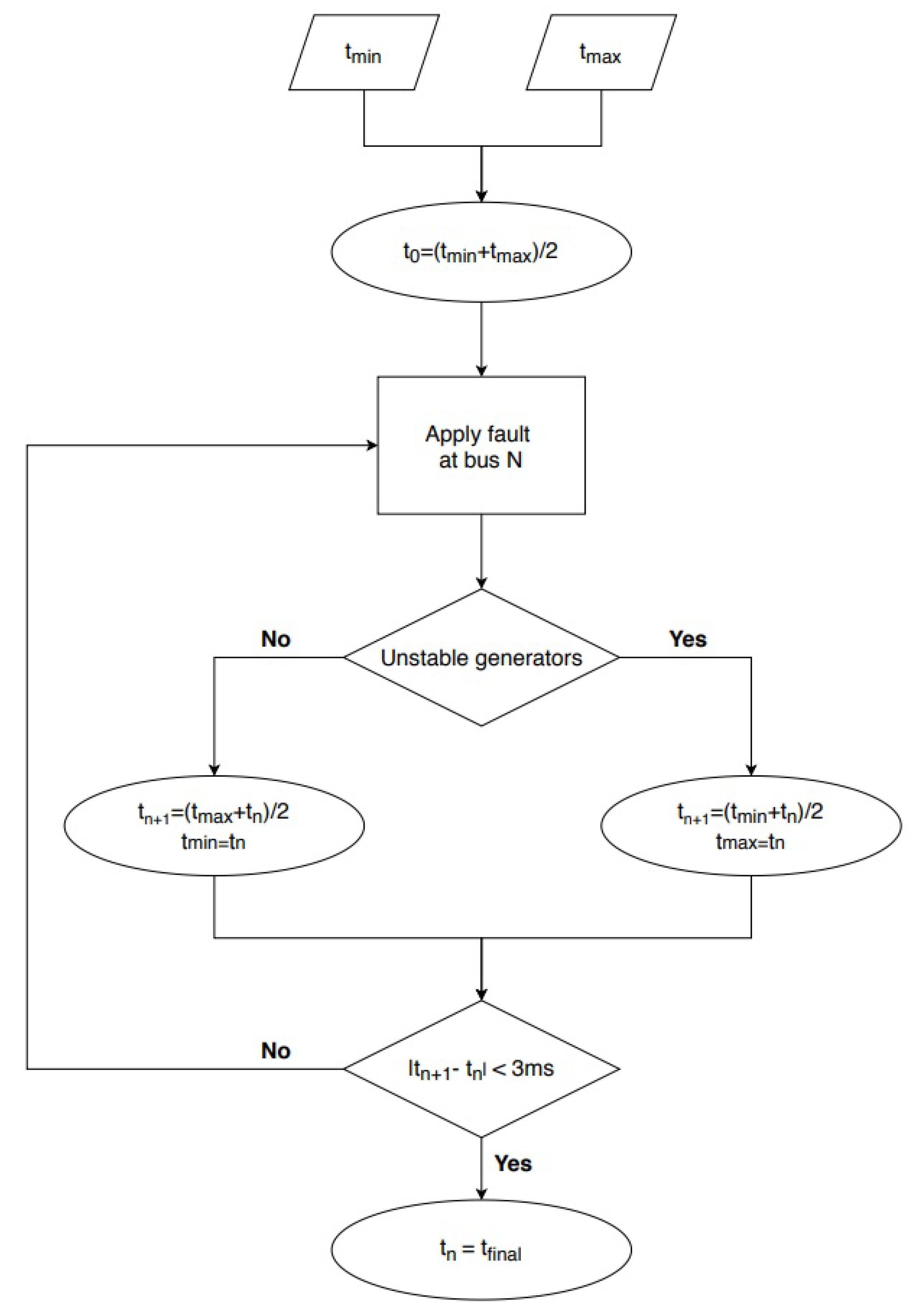
The critical clearing time shall be used to assess the transient stability. The method of determining the critical clearing time with Python 2.7 is shown in the flowchart provided in
Figure 8.
As shown in
Figure 8, there are two inputs for the critical clearing time script i.e.,
and
. These two inputs indicate the time interval in which the simulation will search for the critical clearing time. The first clearing time (
) of the fault is calculated as shown in Equation (
2).
Following this, the fault is applied at a particular bus for
seconds and then the fault is cleared and the simulation continues to run till 5 s. The rotor angles of all synchronous generation units are then scanned to evaluate if the rotor angle exceeds a certain threshold. If there are unstable generators present then the fault clearing time (FCT) is decreased as shown in Equations (
3) and (
4).
If no unstable generators are present then the fault clearing time is increased as shown in Equations (
5) and (
6).
This iterative process is repeated until Equation (
7) holds, yielding the critical clearing time as provided in Equation (
8).
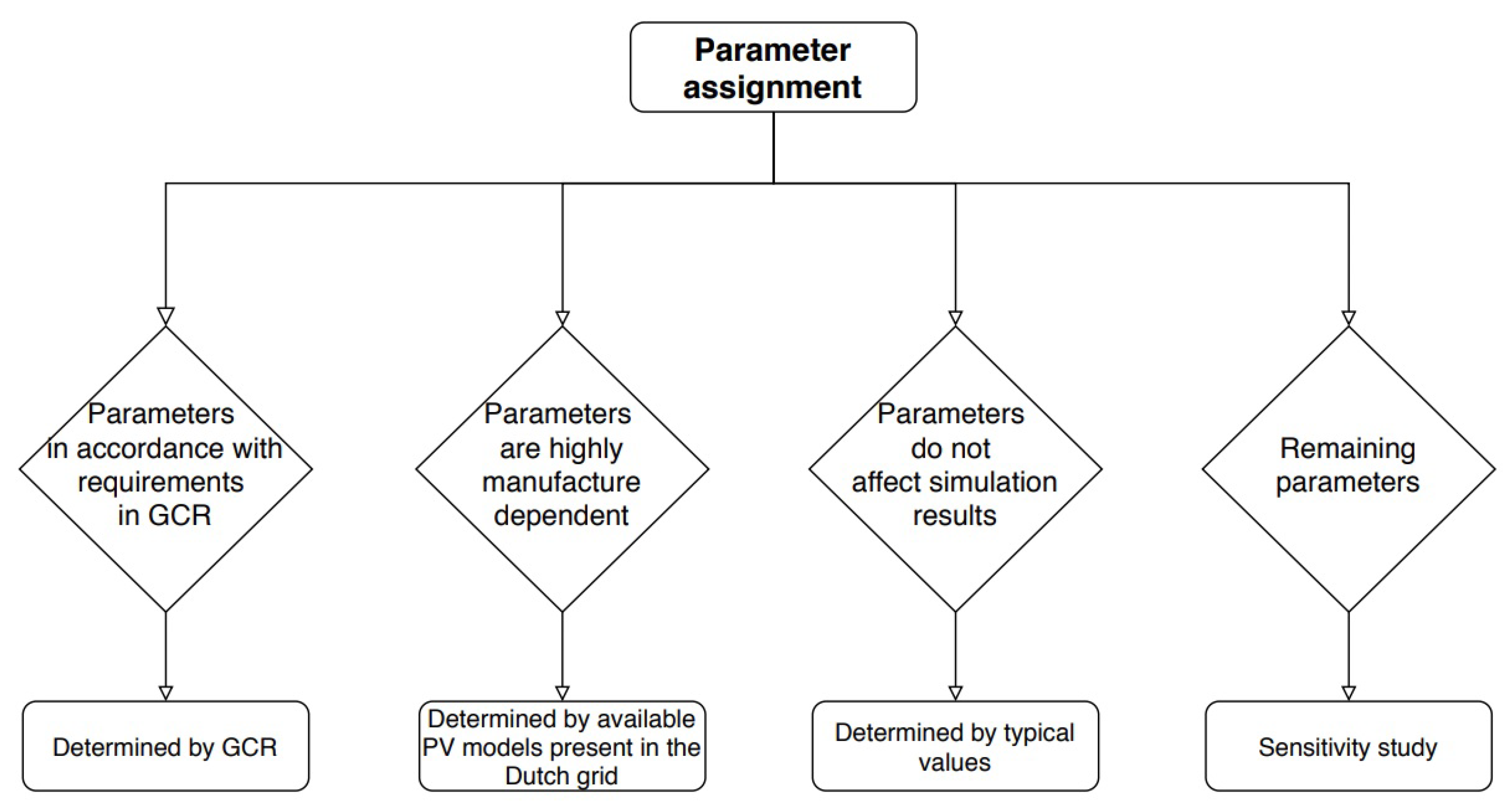
Additionally, for the analysis it is important to define the various methods of PV representation which will be used subsequently. This distinction is made to clearly identify the factors in play which influence the impact of PV penetration on transient stability. The four different modeling representations which shall be studied are:
Representation of all solar PV plants with their respective dynamic models. This representation shall be referred to as All dynamic models.
Representation of all solar PV plants with negative load. This representation shall be referred to as All negative load.
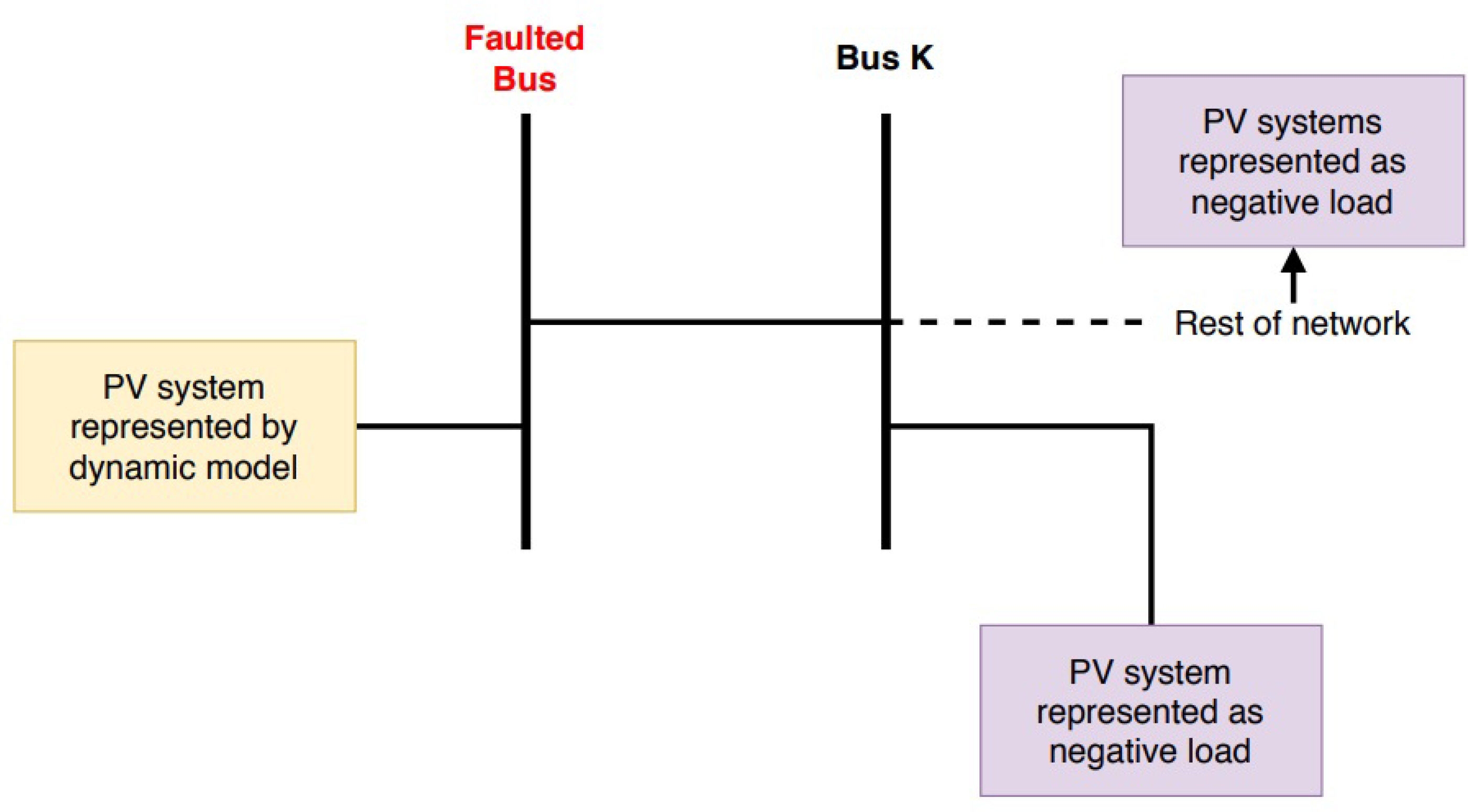
Representation of the solar PV plants connected at the faulted bus with dynamic models while all others are represented by negative load. This representation shall be referred to as Dynamic local 1. A further elaboration of this representation is shown in
Figure 9 (The underlying elements of the PV system have been omitted in the figure for simplicity purposes).
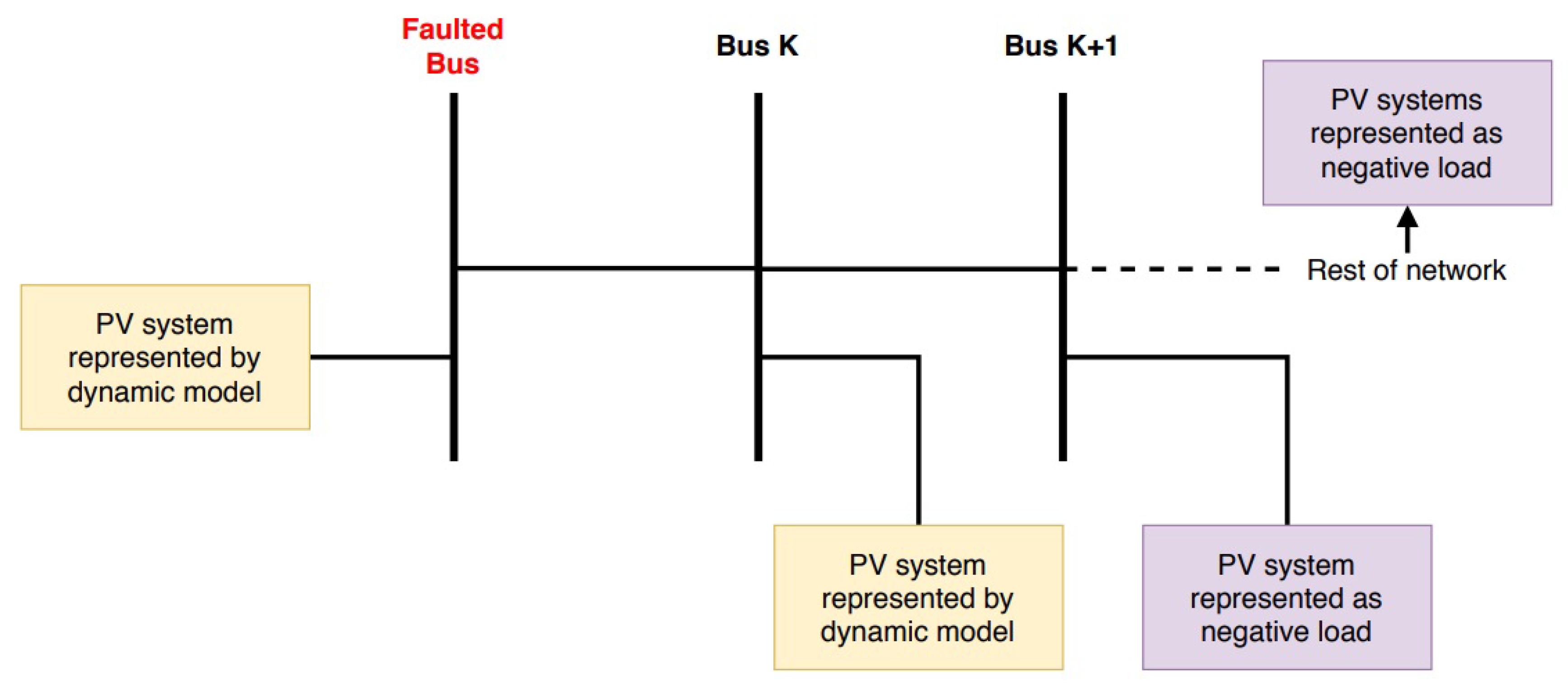
Representation of solar PV plants connected to at the faulted bus and solar PV plants connected at a bus directly connected to the faulted bus are represented with dynamic models. All other solar PV plants are represented with negative load. This representation shall be referred to as Dynamic local 2. A further elaboration of this representation is provided in
Figure 10.
Furthermore, in the figures which shall be discussed, the following abbreviations will be used:
SG — Synchronous generator
A-PV Type A — Aggregated solar PV plants of type A
A-PV Type BCD1— Aggregated solar PV plants of type B, C, D1
L-PV — Large-scale PV system
A-Wind — Aggregated wind systems
3.4. Transient Stability Analysis
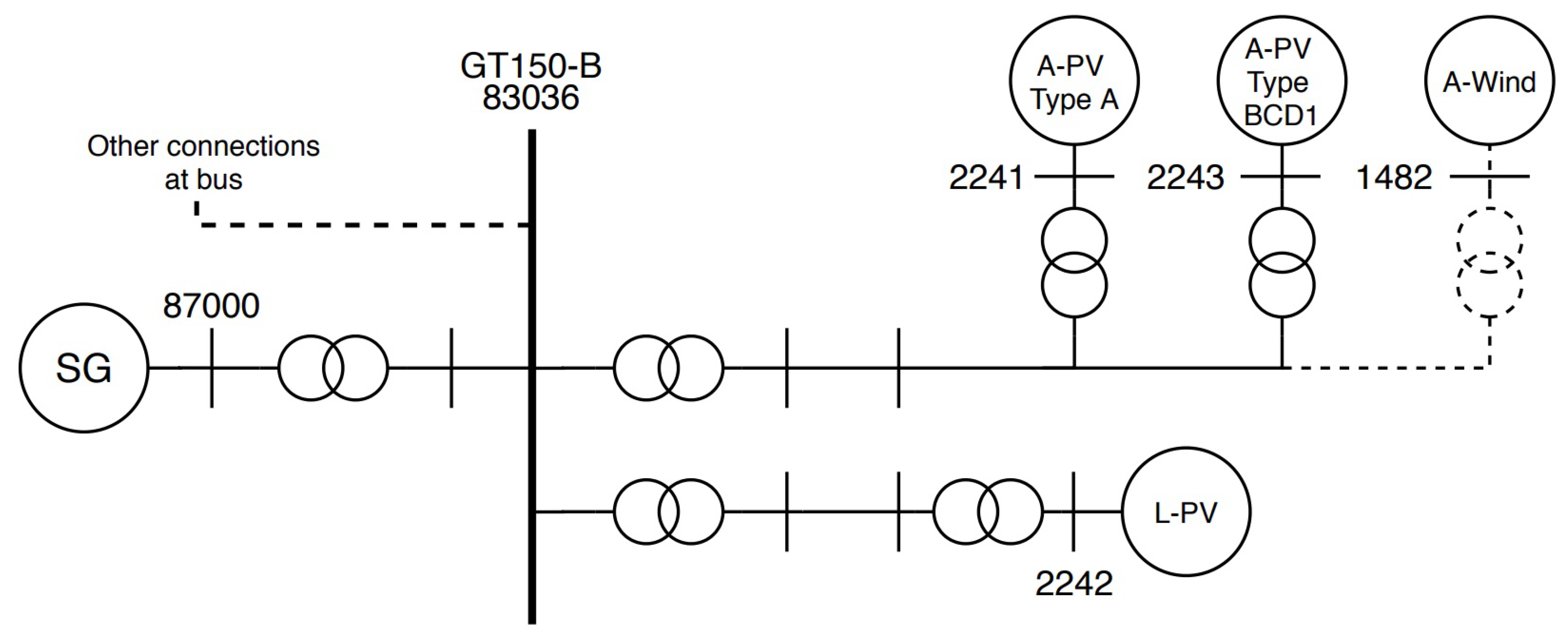
The first bus which will be examined is the bus at Geertruidenberg with a voltage level of 150 kV also referred to as GT150-B. This bus was chosen since there are solar PV plants and a synchronous generator in close proximity. Additionally, the distinction between the short-circuit current (SCC) at this bus can be clearly seen between the various cases. An overview of the relevant connections at this bus is shown in
Figure 11. An aggregated wind system was also connected to this bus, but has been put out of service to solely evaluate the impact of solar PV plants.
To isolate the behavior of short-circuit current on the transient stability, the synchronous generator near the bus of interest (in the case of GT150-B the synchronous generator at bus 87000) has been given a fixed operating point across all cases and the generator bus voltage has been brought within a range of 0.01 pu across all cases. This modification has been made for all the buses which are evaluated. Moreover, the impact of the total system inertia on the transient stability for the different cases is neglected as the network is widely interconnected to European countries and thus the disconnection of certain SGs within the Netherlands has an insignificant influence on the total system inertia. After making the necessary changes as described above in all cases, a fault has been introduced at GT150-B bus 83036 and the critical clearing time for all cases is evaluated and shown in
Table 4.
When first comparing the representation All dynamic models for the different cases provided in
Table 4, it is shown that the critical clearing time is nearly identical for all cases. The minor difference witnessed in case 1 is due to the increased short-circuit current at the faulted bus. Additionally, the difference witnessed in case 4 is due to the reduction of short-circuit current at the faulted bus as several synchronous generators are put out of service for this case. The short-circuit current (calculated with the IEC 60909 method in PSS/E) of the different cases is shown in
Table 5. The equation used to calculate SCC PV ratio in
Table 5 is provided in Equation (
9) and shows the percentage of short-circuit contribution of all the solar PV plants in the network relative to the total short-circuit contribution at the faulted bus.
As shown in
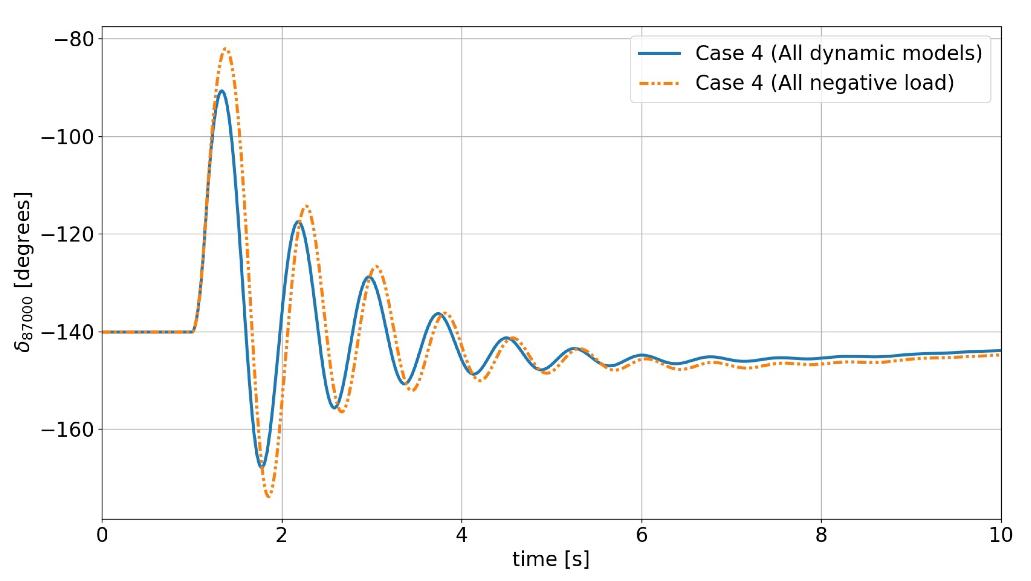
Table 5, the short-circuit current for case 1 is the highest. For this case it is also seen that the SCC PV ratio is the lowest. Hence for the four cases presented, the solar PV plants contribute the least for case 1 relative to the total short-circuit current. This is also reflected when looking at the critical clearing time of case 1 when comparing the representations All dynamic models and All negative load, as the lowest decrease is seen for this case. In other words, the solar PV plants have the smallest effect on the transient stability due to the lowest SCC PV ratio in case 1. Additionally, for cases 2 and 3, similar results are witnessed for the different representations as for these cases the SCC PV ratio is approximately identical. For case 4, a notable decrease in transient stability is seen when comparing the representations All dynamic models and All negative load—the rotor-angle response is provided in
Figure 12, where it is shown that the amplitude of the rotor angle swings for the All negative load case is higher compared to the All dynamic models case. This increased difference stems from the fact that the short-circuit current in this case has decreased (due to out of service of certain synchronous generators) and thus the contribution of the solar PV plants to the total short-circuit current is more prevalent, as indicated by the SCC PV ratio for this case.
From the results provided in
Table 4, it is shown that the solar PV plants do have an effect on the transient stability for this particular bus as the transient stability reduces when removing the dynamic behavior of the solar PV plants. Additionally, it is shown that the impact of the solar PV plants increase when their short-circuit current contribution increases with respect to the total short-circuit current at the faulted bus—this is expressed by an increasing SCC PV ratio.
Furthermore, when comparing the critical clearing time of the various representations, it is shown that the solar PV plants located at the faulted bus and to another bus nearby, do provide a significant contribution to the transient stability, but not a predominant one. As the remaining solar PV plants also aid the transient stability. This distinction between the contribution of local solar PV plants and solar PV plants located electrically further away from the fault is highly dependent on the capacity and the distribution of the solar PV plants in the two different areas.
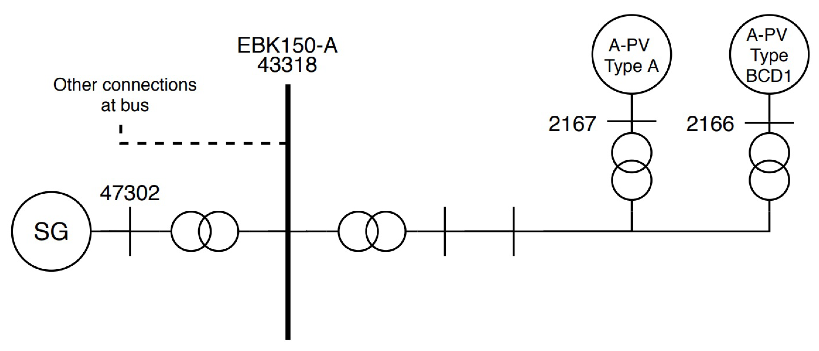
The second bus of interest is Eerbeek abbreviated by EBK150-A. This bus has an aggregated PV system connected and a synchronous generator connected to it but no large-scale PV system. The relevant connections of bus EBK150-A are provided in
Figure 13. Similar to the case study of GT150-B, the synchronous generator close to EBK150-A has been provided with a fixed operating point across all cases and the generator bus voltage has been brought within a range of 0.01 pu across all cases. The critical clearing times for the various cases at this bus are shown in
Table 6.
The results provided in
Table 6 are contrastingly different compared to the results presented for GT150-B. In
Table 6, it is seen that the critical clearing time changes slightly or not at all for the different representations and different cases presented. To obtain better insight as to why this is the case, the short-circuit current at the faulted bus is presented in
Table 7.
First, it is seen that the short-circuit current presented in
Table 7 for the different cases does not vary significantly. From this it can be concluded that the synchronous generators which are out of service for the varying cases do not provide any significant contribution to the faulted bus. Moreover, in
Table 6, it is shown that the critical clearing times vary slightly or not at all for the presented representations and cases. This is due to the fact that the short-circuit contribution of the solar PV plants at this bus is low—this is expressed in the low percentages of the SCC PV ratio. In other words, this area is not populated densely by solar PV plants in close vicinity hence leading to a small contribution to the short-circuit current by the solar PV plants which in consequence leads to the solar PV plants having a limited role in the transient stability for this faulted bus.
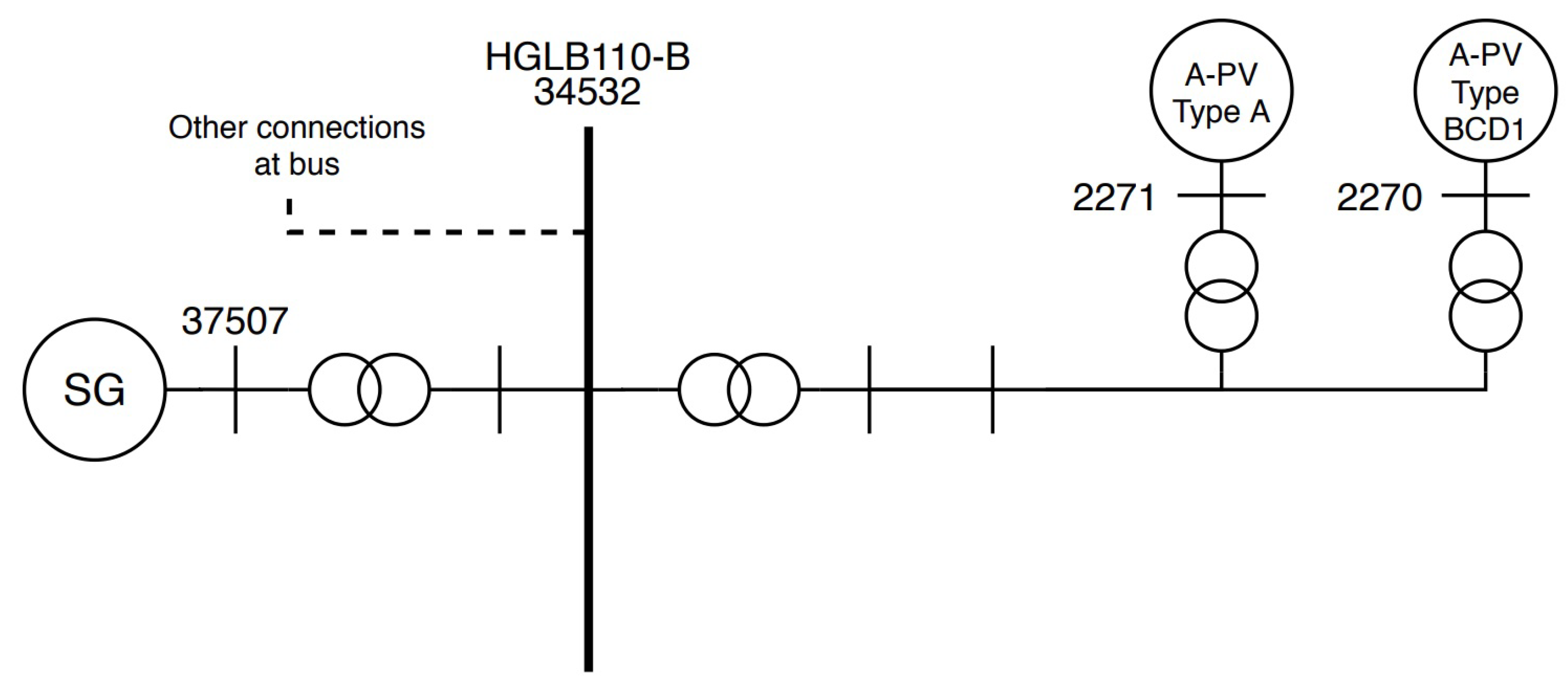
The third case which will be analyzed is the bus at Hengelo Boldershoek at a voltage level of 110 kV, this bus is also referred to as HGLB110-B. An overview of the important connections at this bus is provided in
Figure 14.
The critical clearing times for the four cases are provided in
Table 8. At this bus the representation Dynamic local 1 is equivalent to Dynamic local 2 as no solar PV plants are connected to neighboring buses of bus HNGL110-B.
The results provided in
Table 8 are in line with the results provided for EBK150-A as the critical clearing time contains very minor changes for the various representations. This can explained, again, by looking at the amount of short-circuit current provided in different cases and the amount provided by the solar PV plants as shown in
Table 9.
Similarly as the results provided for EBK150-A, it is shown for a fault at bus HGLB110-B, the critical clearing time is impacted barely by the presence of solar PV plants. For this bus, however, the short-circuit current contribution is higher compared to that seen in EBK150-A. Relative to the total short-circuit current, the average contribution of solar PV plants is slightly less—as expressed by the SCC PV ratios. In similar fashion, the solar PV plants have a limited say in the transient stability at this bus due to the small short-circuit contribution by the solar PV plants.
In the analysis, certain variables which influence the transient stability (e.g., voltage at generator bus, operating point of synchronous generator) were set to fixed values or within a certain range to try and isolate the behavior of solar PV plants on the transient stability. From the analysis it was shown that solar PV plants play an important role in one of the variables affecting transient stability i.e., the short-circuit current at the faulted bus. Two main distinctions in terms of the relation between the total short-circuit current and short-circuit current contribution by the solar PV plants can be made, these are:
High SCC PV ratio—The first distinction which can be made is for a faulted bus which possesses a high SCC PV ratio, this entails that the amount of short-circuit contribution of solar PV plants is high relative to the total short-circuit current at the faulted bus. Such an example was presented when evaluating the bus at GT150-B. In this studied case, the solar PV plants affected the transient stability notably. Additionally, for higher SCC PV ratios as case 4, it was shown that the transient stability was affected the most for this case when removing the dynamic behavior of the solar PV plants as the SCC PV ratio was the highest.
Low SCC PV ratio—The second distinction which can be made is for an area or faulted bus which possesses a low SCC PV ratio, meaning that the amount of short-circuit contribution of solar PV plants is low compared to the total short-circuit current at the faulted bus. Examples of cases with low SCC PV ratios are EBK150-A and HGLB110-B. For these cases it was shown that the low contribution to the total short-circuit current by the solar PV plants led to them having little to no influence on the transient stability.
Looking into the future, power system networks shall continue to phase out synchronous generators and add renewable energy sources such as solar PV plants. Consequently, the short-circuit current in the various regions shall decline as synchronous generators provide significantly more short-circuit current compared to renewable energy sources. This overall decline in short-circuit current and increase of short-circuit current contribution by solar PV plants shall progress a lot of areas towards higher SCC PV ratios and thus solar PV plants (and other RES) shall have a continuingly increasing influence on the transient stability.
The remarks above state the impact which solar PV plants have on the transient stability. It is also important to highlight when significant decrease in transient stability is witnessed. If the total short-circuit current at a faulted bus is highly contributed by synchronous generation units, then for certain situations in which synchronous generation units are put out of service, the short-circuit current at such a bus might decrease significantly henceforth potentially leading to harmful effects for the transient stability. Also, if a fault occurs at a bus near a synchronous generation unit which contains a low short-circuit current, transient stability problems might arise when such a synchronous generation unit is operating at a high operating point (close to its active power limit and under-excited).
3.5. Improving Transient Stability
In this section, methods to improve transient stability shall be proposed. The methods which will be discussed are:
Limiting operation region of synchronous generator
Addition of reactive compensation devices
Decreasing reactance between synchronous generator and faulted bus
Operating point of synchronous generator: The operating point of the synchronous generator plays an important role in the transient stability. To illustrate this point, GT150-B shall be evaluated (connections at this bus are shown in
Figure 11) and the operating point of the synchronous generator nearby will be varied. To examine the impact of operating point of the synchronous generator on the transient stability, case 2 has been used. The maximum active power output (Pmax) and the MVA base of the generator at bus 87000 near GT150-B are equal to 650 MW and 812.50 MVA, respectively. The different operating points and the respective critical clearing times are provided in
Table 10.
In
Table 10, it is seen that the critical clearing time for operating point 1 till 3 yields the lowest critical clearing times compared to the other cases. For these operating points only the reactive power output of the synchronous generator has been varied, while the active power output is close to its limit. These operating points yield the lowest critical clearing times because the rotor angle is at a higher operating point yielding less margin for transient stability. In these cases, it is due to the high amount of active power being generated relative to the Pmax of the generator. Additionally, it is also seen that the critical clearing time for operating point 3 is the worst. Thus, the synchronous generator is at its most critical when a combination of high amount of active power generation and an under-excited generator is present. Similar conclusions can be drawn when looking at operating point 4 and 5, where it is seen that the under-excited generator decreases the critical clearing time significantly. On the other hand, it is seen that the active power generation is not as high compared to operating points 1 till 3 and hence the critical clearing time is not as low. Concludingly, it is illustrated that the transient stability is highly dependent on the operating point of the synchronous generator. Furthermore, the operating point of the generator has the most significant effect on the transient stability when the active power generation is close to its limits and the generator is under-excited. Consequently, for critical areas where synchronous generators are in danger of losing synchronism, limitations can be set on the synchronous generators near such relevant areas regarding the active power production and reactive power output to improve the transient stability.
Addition of reactive compensation device: As shown in the analysis, the short-circuit current at the faulted bus has a significant say in the transient stability. To illustrate this phenomenon, case 2 at the bus of EBK150-A is looked at without and with the addition of a reactive compensation device. The reactive compensation device has been added to the high voltage bus, in this case bus EBK150-A. The added reactive compensation device has a rating of 500 MVA. The critical clearing time of these two cases is shown in
Table 11.
As shown in
Table 11, the critical clearing time for the case with reactive compensation device has increased compared to the case without. This is due to the added short-circuit current contribution of the added device. An example of such devices are synchronous condensers or static compensators (STATCOM). Conclusively, it was shown that by adding a reactive compensation device such as a synchronous condenser or STATCOM, the total short-circuit current at the faulted bus increases hence improving the transient stability. Additionally, such devices also contribute to the voltage support.
Decrease reactance: Another method to improve the transient stability, albeit a very cost intensive one, is decreasing the reactance of the lines/cables or transformer in between the critical synchronous generator and the faulted bus. To demonstrate this point, bus GT150-B and case 2 has been looked at. A modification has been made by decreasing the reactance of the line between the synchronous generator at bus 87000 and the faulted bus GT150-B. The initial and modified reactance and the obtained critical clearing times for the two cases is provided in
Table 12.
As shown in
Table 12, by decreasing the reactance between the synchronous generator and the faulted bus, the critical clearing time increases. This can be explained by looking at the power flow transfer equation shown in Equations (
10) and (
11).
As shown in Equations (
10) and (
11), the reactance is inversely proportional to the amount of active and reactive power transferred. Hence, when decreasing the reactance of the line from the synchronous generator to the faulted bus, less losses occur in terms of reactive power when the reactance is decreased, hence leading to a higher short-circuit contribution at the faulted bus and thus improving the transient stability. Realistically, this can be achieved by two methods,
By replacing the line/cable from the synchronous generator to the faulted bus with a line/cable with lower reactance. This alternative is very costly and does not provide any direct benefits other than an improved robustness and transfer capacity of added line. However, since the line will be completely replaced, the replacing line/cable can yield a low reactance.
By adding a parallel line from synchronous generator to the faulted such that the equivalent reactance is hence decreased. This alternative offers redundancy and the ability to spread the transfer over two lines. However, as the equivalent reactance is also a function of the existing line/cable, this poses a limitation for the decrease in equivalent reactance.


 ,
, 


