

Effect of a Large Proton Exchange Membrane Electrolyser on Power System Small-Signal Angular Stability

Mechatronic, Electrical Energy, and Dynamic Systems, UCLouvain, 1348 Louvain-la-Neuve, Belgium
*
Authors to whom correspondence should be addressed.
Electricity 2023, 4(4), 381-409; https://doi.org/10.3390/electricity4040021
Submission received: 5 October 2023
/
Revised: 3 November 2023
/
Accepted: 13 November 2023
/
Published: 1 December 2023
(This article belongs to the Topic Power System Dynamics and Stability)
Abstract
:The dynamics of electrical systems have changed significantly with the increasing penetration of non-conventional loads such as hydrogen electrolysers. As a result, detailed investigations are required to quantify and characterize these loads’ effects on the dynamic response of interconnected synchronous machines after being subjected to a disturbance. Many studies have focused on the effects of conventional static and dynamic loads. However, the impact of hydrogen electrolysers on the stability of power systems’ rotor angles is rarely studied. This paper assesses the effect of proton exchange membrane (PEM) electrolysers on small-disturbance rotor-angle stability. Dynamic modelling and the control of a PEM electrolyser as a load are first studied to achieve this. Then, the proposed electrolyser model is tested in the Amercoeur plant, which is part of the Belgian power system, to study its effect on the small-signal rotor-angle stability. Two approaches are considered to examine this impact: an analytical approach and time-domain simulations. The analytical approach consists of establishing a state-space model of the Belgian test system through linearisation around an operating point of the non-linear differential and the algebraic equations of the synchronous generators, the PEM electrolyser, the loads, and the network. The obtained state-space model allows for the determination of the eigenvalues, which are useful to evaluate the effect of the PEM electrolyser on the small-signal rotor-angle stability. This impact is investigated by examining the movement of the eigenvalues in the left complex half-plane. The obtained results show that the PEM electrolyser affects the electromechanical modes of synchronous machines by increasing their oscillation frequencies. The results also show that the effect of the electrolyser on these modes can be improved by adjusting the inertial constant and the damping coefficient of the synchronous machines. These results are consolidated through time-domain simulations using the software Matlab/Simscape from the version MatlabR2022a-academic use from Mathworks.
1. Introduction
Nowadays, hydrogen demand and production in a multitude of sectors are constantly increasing. As a result, the number of hydrogen electrolysers connected to transmission power systems is increasing. Hydrogen electrolysers are electrochemical devices used to separate water molecules into hydrogen and oxygen by passing a DC current through them [1]. This DC current is proportional to the hydrogen production. There are different hydrogen electrolyser technologies, which range from small systems (kilowatts) to large-scale systems (multiple megawatts) [1]. The most well-known technologies in industrial projects under development are alkaline electrolysers and proton exchange membrane (PEM) electrolysers [2]. Alkaline electrolyser technology, which is widely used today, is considered a mature technology in the industrial sector. Due to their advantages over alkaline electrolysers, such as high power density and cell efficiency, as well as fast dynamics, PEM electrolysers are in a period of great expansion and development for integration into power systems, including renewable energy production systems [1,2,3,4,5]. For this reason, PEM electrolyser technology is dealt with within this paper. Hydrogen electrolysers can be viewed as flexible loads that can facilitate the large-scale integration of intermittent renewable sources into future power systems and provide power grid services [6,7]. As loads, hydrogen electrolysers can have an impact on the dynamics and stability of power systems. The use of power electronic converters as an interface for their integration into the grid can also affect the power quality and dynamics of power systems [8,9]. In addition, the dynamic response of the required electrolyser current to produce hydrogen can influence the dynamics of power systems. Detailed investigations of the impact of hydrogen electrolysers are required to characterize the dynamic response of the rotor-angle stability, frequency stability, and voltage stability. However, the majority of studies have focused mainly on frequency stability [3,5,6,10] and technoeconomical aspects [10]. Few articles have dealt with the effect of hydrogen electrolysers on voltage stability [10], and the impact of electrolysers on rotor-angle stability has rarely been studied.
This paper focuses on the impact of a large-scale PEM electrolyser on a power system’s small-signal rotor-angle stability. The small-disturbance rotor-angle stability can be defined as the capacity of a set of interconnected synchronous machines to maintain synchronism after being subjected to a small disturbance [11]. The dynamic responses of the set of interconnected synchronous machines are quantified and characterized to assess the influence of the PEM electrolyser on the power system dynamics. To this end, a large-scale PEM electrolyser project within the Belgian power system around Amercoeur is considered as a test system. Before investigating the effect of a hydrogen PEM electrolyser on the small-signal rotor-angle stability, we first identify the nature of PEM electrolysers when they are considered as loads within the power system, that is, whether a hydrogen PEM electrolyser can be regarded as a constant impedance load, a constant current load, or a constant power load. To achieve this, it is necessary to first model a hydrogen PEM electrolyser, then model the power electronic converter, and, finally, to develop a control structure for the power electronic converter to adjust the electrolyser current.
Concerning the dynamic modelling of PEM electrolysers, various electrochemical models are proposed in the literature [2,12,13,14]. The authors of reference [2] developed a dynamic electrical model of a PEM electrolyser, taking into account the dynamic behaviour of the PEM electrolyser during sudden variations in the input current. An equivalent electrical model of the PEM electrolyser with adaptive parameters for both static and dynamic operating conditions was proposed in [12]. The study reported in [12] focused on modelling cell voltage as a function of static and dynamic operations. In [14], an analytical–dynamic analysis model for a PEM electrolyser deduced from physical laws and electrochemical equations was proposed. The dynamic modelling of PEM electrolysers, as described in the literature, can be categorized into four groups based on various physical aspects, such as the required voltage (reversible voltage) for the electrolysis [15,16], activation overpotential, ohmic resistance, and the diffusion aspects at both the anode and the cathode. The activation overpotential represents the electrochemical kinetic behaviour [17]. It is therefore a representation of the speed of the reactions taking place on the electrode surface [17]. In contrast, ohmic overpotential is caused by the ohmic resistance of the electronic materials, such as current collectors, bipolar plates, and electrode surfaces [17]. It includes electron and proton conduction through the PEM. The electrochemical model of the PEM electrolyser investigated in [2,4,12,14,17] is referred to as the first model (Model 1) in this paper. is composed of the activation overpotential at the anode and cathode, membrane overpotential, and reversible potential. The activation overpotential at both the anode and cathode is modelled by two capacitor-resistance branches. Furthermore, the membrane overpotential is modelled by the ohmic overpotential. Model 1 is one of the most studied models in dynamic modelling analysis of electrolysers. Nevertheless, its dynamic behaviour is often not studied. The second model () considered in this paper includes a Warburg impedance at both the anode and the cathode, as proposed in [10]. The Warburg impedance is related to the concentration losses in the PEM electrolyser and is more important at low frequency and high current density [18,19]. However, dynamic modelling of the electrochemical model related to is not proposed in the literature. Other authors have neglected the activation overpotential at the cathode, as in [3,4,8,10]. This is because the contribution of this overpotential is considered small compared to the contributions of the activation overpotential at the anode, the ohmic overpotential, and the reversible voltage. As a result, the electrochemical model without the activation overpotential of the cathode can be classified as either a model with a Warburg impedance () or a model without a Warburg impedance (). The electrochemical model with Warburg impedance is often modelled by a Rangdles–Warburg cell, as depicted in [10,20]. includes a frequency-dependent Warburg element, which is parallel to a conventional capacitor, and a conventional resistor, which is in series with the Warburg element. The Warburg model brings the frequency-dependent characterizations of the resistor and capacitor, which modify the dynamic response of the cell voltage. , which does not consider the Warburg impedance, is described in [3,4,8]. As with the first two electrochemical models presented previously, the dynamic behaviour of the last two electrochemical models is also not examined in the literature. The dynamic responses of four models proposed in the literature are studied in this article in order to choose which one can be used in load modelling and small signal modelling. This choice is dictated by the time constant that characterizes the dynamic response of each model. For the model of the hydrogen PEM electrolyser, the temperature and pressure are considered to be constant, and the degradation of the catalyst and the membrane is not taken into account.
A 12-pulse thyristor rectifier is often used as interface to integrate hydrogen electrolysers into the grid. Because this technology is one of the most mature and important solutions in high-power rectification applications [8], a current control structure is proposed to adjust the appropriate firing angle to achieve the desired electrolyser current. The proposed current control structure is established based on a dynamic model of the average model of the thyristor rectifier and of the proposed hydrogen PEM electrolyser model.
Finally, the effect of the PEM electrolyser model on the small-signal rotor-angle stability is studied using a state-space model and time-domain simulations of the test transmission system. The proposed state-space model is based on linearisation around an operating point of the non-linear differential and algebraic equations of the synchronous generators, the distribution network, the conventional loads, and the PEM electrolyser. In this approach, the synchronous generators and the network are modelled in the synchronous reference frame. Then, all the components within the transmission network are translated into the common synchronous reference frame, rotating at a common frequency, as described in [21]. As well as consolidating the analytical results, time-domain simulations are also employed in this paper to study the impact of the proposed modelling of the electrolyser as a load. The contributions of this study can be summarized as follows:
- A dynamic model and a state-space model of a system formed by a PEM electrolyser and a 12-pulse thyristor rectifier is proposed.
- A control structure for the electrolyser current from the dynamic model of the PEM electrolyser and for the average model of the 12-pulse thyristor rectifier is proposed.
- A model of the PEM electrolyser as a load is proposed to identify whether it can be considered a constant impedance load, a constant current load, or a constant power load.
- We study the effects of the PEM electrolyser on the stability of the small-signal rotor-angle using analytical and time-domain simulation approaches.
The remainder of this paper is organized as follows: Section 2 presents the details of the proposed dynamic model for the PEM electrolyser, the thyristor rectifier, the proposed control structure of electrolyser current, and the modelling of the electrolyser as a load. Section 3 presents the details of the proposed small-signal model of the Belgian test system, while the stability analysis results are presented in Section 4. Finally, Section 5 concludes the paper.
2. Power System Architecture and Integration of Hydrogen PEM Electrolyser
Figure 1 describes the used test system, in which 100 MW of PEM electrolysers are connected to the 150 kV busbar. It is the topology corresponding to the Belgian power system around the Amercoeur power plant. It consists of three synchronous generators () connected to the transmission grid through main 4, 6, and 11. The are round rotor machines with static exciters. The three are coupled with the thermal power plants. The dynamic of the primary source coupled with the is not studied in this article. It is assumed that the three operate with constant power generated by the primary source. They are modelled as nodes with fixed active power (P) and reactive power (Q) (). The 270 MW synchronous generator () is connected to Busbar 4, to which the PEM electrolyser is connected. The 150 MW generator () is connected to the electrolyser via and , while the 410 MW synchronous generator ) is connected to the electrolyser through , , and . A large 100 WM PEM electrolyser is connected to . The large-scale PEM electrolyser is assumed to be viewed as a large load by the power system, consuming only active power.
2.1. Dynamic Modelling of the PEM Electrolyser
In order to model an electrolyser as a whole, it is necessary to look at each of its constituent aspects, such as electrochemical, electrical, thermal, mass transfer, and fluid [22] components. This paper focuses only on the electrochemical and electrical models.
Various electrochemical models of PEM electrolysers have been proposed in the literature [2,3,8,10,12,13,14,20], which can be categorized into four groups, as discussed in the introduction: , , , and . The performance of each model can be quantified by evaluating the dynamic response of the cell voltage for a fixed cell current. The dynamic behaviour of these four electrochemical models is obtained by the following equations:
- : Classical electrochemical model without Warburg impedance.
This model is described in [2,4,12,13,15,16], and the cell voltage across a PEM stack is given by
where and are the activation overpotential at the anode and at the cathode, respectively; represents the input current of the cell; and and are the ohmic resistance and reverse voltage potential (reversible potential), respectively, during the water-splitting reaction. The dynamic behaviour of this classical electrochemical model is imposed by , and it is modelled by:
where represents the double layer capacity, and and are the charge transfer resistances at the anode and cathode, respectively, which are temperature-dependent.
- : Classical electrochemical model with a Randles–Warburg cell.
This electrochemical model is presented in [10]. Its dynamic model is given by:
where denotes the Warburg impedance, which is frequency-dependent. Its mathematical expression is given as follows [19]:
where , , and are the diffusion resistance and charge transfer resistance, respectively, and , and represent the diffusion time constant and double layer capacitance, respectively.
- : Electrochemical model without the activation overpotential of the cathode and with Randles–Warburg impedance.
This model is presented in [10,20]. Without the activation overpotential at the cathode, the cell voltage across the PEM stack is modelled as follows:
The dynamic model of activation overpotential at the anode is modelled as in Equation (5).
- : Electrochemical model without activation overpotential at the cathode or a Warburg cell.
This model is depicted in [4,8]. The dynamic model of the cell voltage across the PEM electrolyser as a function of the activation overpotential at the anode is given by Equations (5) and (7). For a cell current set to 5 A, the dynamic responses of the cell voltages of l, 2, 3, and 4 from Equations (1)–(7) are described in Figure 2. The used cell parameters and Randles–Warburg cell parameters of those models are given in [10,18].
Figure 2 shows that the four electrochemical models can be identified in two groups: models without activation overpotential of the cathode ( and ) and complete models ( and ). For each group, we can identify models with Warburg impedance ( and ) and those without Warburg impedance ( and ). The impact of Warburg impedance on the cell voltage is also observed through the voltage deviation between and and that between and . Furthermore, the difference in voltage between the two groups is around 0.182 V, which represents the cathode activation overpotential. This overpotential is smaller than the total cell voltage, which is close to 2.055 V for and and around 1.872 V for and under steady-state conditions. This may be the reason why some authors neglected this cathode activation overpotential in their models [10].
Additionally, Figure 3 shows that the cell voltage responses of electrochemical models with Warburg impedance ( and ) are close to those without Warburg impedance ( and ). However, their transient response is higher than that of and . This is illustrated by the time constant, which is higher for and than for and .
From these results, it can be concluded that the dynamic response of electrochemical models with a Warburg impedance (or a Randles–Warburg cell) is close to that of those without a Warburg impedance. Nevertheless, Warburg impedance can introduce a larger time constant in the transient response, and it can make the dynamic modelling of the electrochemical model more complex. Therefore, is used for the rest of this paper. offers a better transient response compared to the other models (see Figure 3).
2.2. Modelling of the 12-Pulse Thyristor Rectifier and the Electrolyser Current Controller
Figure 4 shows a hydrogen PEM electrolyser model connected to the grid through a 12-pulse thyristor rectifier and a three-winding wye-wye-delta transformer. The PEM electrolyser is modelled by the electrochemical model as described in the previous subsection. The three-winding transformer has the ability to eliminate the 5th-and 7th-order harmonic currents [8]. The electrolyser model is connected to the rectifier bridge via a filter inductance () and interphase inductances (). The two 6-pulse thyristor rectifiers connected in parallel are used to form a 12-pulse thyristor rectifier. This configuration is often considered to be one of the most mature solutions for high-current rectification applications [8]. The operation of each six-pulse rectifier is ensured by a firing angle () that is either specified or generated by a controller, depending on the desired response of the rectifier DC side. Figure 4 also highlights that the transfer of active power () from the AC side to the DC side () is ensured by an appropriate firing-angle signal. The DC voltage and DC current are also related to the firing angle generated by the current controller from the current set point and the measurements of the DC current signal () and the AC voltage signal (). can be measured at the primary or secondary end of the three-winding transformer. It is used by the phase-locked loop (PLL) to synchronize the electrolyser with the grid frequency.
2.2.1. Electrical Model of the 12-Pulse Thyristor Rectifier
Establishing the dynamic model shown in Figure 4 requires that all the parameters and variables on the AC side of the rectifier be brought back to the DC side. To do this, the average model of a 12-pulse thyristor rectifier can be considered. Additionally, the transformer is modelled by the primary and secondary leakage inductances.
Considering that the primary end of the transformer is supplied by , this voltage can be seen by the electrolyser through the DC voltage using the following expression:
where is the RMS phase-to-phase voltage at the primary end of the transformer, and k represents the ratio between the RMS phase-to-phase voltage at the secondary end of the transformer () and that at the primary voltage (). Finally, corresponds to the firing angle.
Equation (8) shows that the DC voltage is a function of the firing angle. It shows that the maximum voltage can be obtained when the firing angle is equal to zero. We assume that the transfer of current between two consecutive thyristors in a commutation group takes a finite amount of time (overlap time). This overlap time depends on the phase-to-phase voltage between the thyristors participating in the commutation process, as well as the leakage inductance between the thyristor rectifier and the AC grid [23]. During the overlap time, the voltage and the current on the DC side are given by [23]:
where is the leakage inductance of the transformer, and is the overlap angle. Equations (9) and (10) allow for the establishment of an equivalent circuit of the thyristor rectifier converter, as shown in Figure 5. The converter is modelled by a voltage source in series with a virtual resistance, whereas the overlap time phenomenon is modelled through the equivalent resistance given by . Note that this resistance is not real (virtual resistance) because it does not dissipate power [23].
The dynamic model of the 12-pulse thyristor rectifier associated with the PEM electrolyser can be obtained from Figure 5 by applying Kirchhoff’s law. The resulting model is defined as:
2.2.2. Control Structure Model for the Electrolyser Current
The current control structure can be obtained from the dynamic model that is described by Equations (11) to (13). By applying Laplace transform to these equations and setting the initial conditions of current () and activation voltage () to zero, the following is obtained:
A block diagram of the system based on Equations (14) to (16) is shown in Figure 6. It describes the dynamic model of the PEM electrolyser associated with the 12-pulse thyristor rectifier in the s domain. This model is composed of two subloops of current and voltage, as well as signals of reverse voltage () and DC input voltage ().
The proposed cell voltage control structure from the physical system model (Figure 6) is depicted in Figure 7. It consists of an internal current control loop and an external voltage control loop. The feed-forward terms ( and ) are added at the output of the DC current control loop to compensate for the opposite signals of physical signals of and .
The proposed control structure (Figure 7) is general. It can be used to control both cell voltage and cell current. To control the DC current, the DC current control loop structure is used (light blue), whereas the DC voltage loop control structure including the blue part is used to control the cell voltage.
The implementation of the current control structure given in Figure 7 requires a phase-locked loop (PLL) to synchronize the electrolyser with the grid frequency. The main function of the PLL is to track the phase () of the voltage, which is the voltage node to which the electrolyser is connected (see Figure 1). This phase can be expressed by under steady-state conditions, where is the pulsation corresponding to the reference frequency of the grid. The control structure of the PLL is described in [24].
The steady-state conditions of 100 MW of PEM electrolysers connected to (see Figure 1) are given in Figure 8. We consider the proposed current control structure and parameter values of the test grid and interpolate parameter values of the PEM electrolyser from [10,18] to those of the 100 MW PEM electrolyser. The DC electrolyser current is given in Figure 8a. The firing angle is depicted in Figure 8b. The DC voltage is presented in Figure 8c. The computed steady-state conditions are 21,790 A, 4588 V, and . The results were obtained using the parameters shown in Table 1 [10,18] and the current control structure illustrated in Figure 8. Figure 8 also shows that the proposed controller is also able to reach another steady-state operating point after changing the electrolyser current set point, for example, by changing the electrolyser current set point by at 6 s, i.e., from 21,790 A to 21,576 A. The controller maintains the DC current at the desired value (see Figure 8a). The firing angle increases (Figure 8b) to decrease the DC voltage (Figure 8c).
2.3. Modelling of the PEM Electrolyser as a Load
Consider the PEM electrolyser modelled in Figure 4, which is detailed in Figure 5. If one considers just the electrolyser part in Figure 5, the cell voltage of the stack is given by Equation (12). The activation voltage () is essentially caused by the voltage associated with the transfer resistance () because the current on the capacitance is equal to zero. Therefore, one obtains:
If it is assumed that there are no power losses between the grid and the electrolyser—that is to say that the active AC power supplied by the grid is equal to the DC power consumed by the hydrogen electrolyser—the power consumed by the electrolyser can be calculated as:
Equation (18) shows that equivalent resistance () and reversible potential () are constant. This yields the active power () as a function of the DC current (). is constituted by two active power terms ( and ). The first element varies directly with the square of the current, while the latter varies with the current. In contrast to traditional static load modelling, the whole active power is modelled as a function of voltage magnitude. Since it is assumed that the DC voltage is fixed by the grid voltage to which the electrolyser is connected, the proposed modelling of the PEM electrolyser as load can be based on the controlled DC current. Thus, the PEM electrolyser can be modelled as a function of the cell current. According to Equation (18) and Figure 4, the PEM electrolyser can be modelled as a fraction of a constant impedance load combined with a fraction of a constant current load. The proposed model is expressed by Equation (19). In contrast to the conventional exponential ZIP model [25,26], the proposed model is modelled as a function of the current ratio instead of the voltage ratio. This makes the proposed load model of the electrolyser different from that of conventional constant impedance and constant current loads.
where is the rated active power of the electrolyser, represents the nominal DC electrolyser current related to the nominal active power of the electrolyser, is the controlled current of the electrolyser, represents the fraction of constant impedance load, and is the fraction of the constant current load.
Note that the modelling of the electrolyser as a load may depend on the model of the electrolyser, the technology of the power electronic converter, and the way in which the electrolyser is connected to the grid. For a technology based on a single 12-pulse thyristor rectifier with n electrolysers connected in parallel on the DC side, as illustrated in Figure 9, the factor decreases with an increase in the number of parallel connected electrolyser models. Consequently, the PEM electrolyser behaves as a constant-current dominant load. Otherwise, it behaves as a constant-impedance dominant load.
Equations (18) and (19) and Figure 9 and Figure 10 illustrate an example of the variation of fractions of a constant impedance load () and constant current load () depending on the number of electrolysers connected in parallel to the DC rectifier side. Four possibilities of connecting a 100 MW PEM electrolyser to the DC side of the 12-pulse thyristor rectifier are proposed. When one 100 MW PEM electrolyser model is connected to the DC side, Figure 10 shows that the fraction of constant impedance load () is higher than that of the constant current load (). Therefore, the PEM electrolyser model can be seen by the grid as a dominant constant impedance load, whereas when two 50 MW PEM electrolysers are connected in parallel, this can be considered a dominant constant current load. For four models of 25 MW each connected in parallel, the fraction of constant impedance load () is higher than that of the constant current load (). The PEM electrolyser can be assimilated to a dominant constant current load.
3. Small-Signal Modelling of the Test System
Small-signal analysis was used as a tool to investigate the effects of the PEM electrolyser on the small-signal angular stability, i.e., to investigate the impact of the PEM electrolyser on the capacity of a set of interconnected synchronous machines to maintain synchronism after being subjected to a small disturbance. To do this, the power system shown in Figure 1 can be described by a system of non-linear differential and algebraic equations. Then, it is linearised around the operating point to obtain the state-space model of the grid. Hence, the state-space model of the grid shown in Figure 1 has to be established. It is composed of small-signal submodels of synchronous machines (270 MW, 150 MW, and 410 MW), static exciters, the PEM electrolyser, the network, and loads. Such equations can be written as follows.
3.1. State-Space Model of Synchronous Generators
The state-space model was obtained by the linearisation of non-linear differential and algebraic equations of the synchronous machines around an operational point. The rotor and stator equations are established in the reference frame (via Park transformation) [11,21]. The differential equations in the synchronous reference frame of each synchronous machine connected to the grid are described by [21]:
where i = 1, 2, and 3 correspond to the number of the synchronous generator (, , and , respectively) connected to the test system; is the synchronous angular speed of the rotor; and and are the rotor speed and relative rotor angle, respectively. The rotor angle () is measured with respect to the synchronously rotating frame of the constant base frequency () and satisfies [27]. is the mechanical torque. is the damping torque coefficient. represents the inertial constant. and are the current components along the direct axis (d axis) and quadrature axis (q-axis), respectively. and are the synchronous reactances along the d axis and q axis, respectively. and are the transient time constants along the d axis and q axis, respectively. and represent the transient reactances along the d axis and q axis, respectively. is the field voltage. represents damper-winding () flux linkages. is the damper-winding () reactance. and are the magnetizing reactances in d-axis and q-axis, respectively. is the field d-axis reactance. is proportional to the rotor field flux along the d axis, while is proportional to the damper-winding flux along the q axis.
Each synchronous machine of the test system is composed of a static exciter to maintain a constant terminal voltage. The dynamic model of the static exciter is expressed according to the following equation [21]:
The real parts of the equations of the stator for each synchronous generator (, , 2, and 3) are given by [21]:
To obtain a linearised model for Equations (20)–(26), a small perturbation around the operating point is superimposed on the state variables , , , , , , , , , , and , such as:
where , , , , , , , , , , and represent the nominal values of the rotor angle, rotor speed, damper winding flux, rotor field flux, field voltage, q-axis current, d-axis current, terminal voltage of the , reference voltage of the exciter, mechanical torque, and voltage angle at bus i, respectively. , , , , , , , , , , and are the small disturbances of the state variables mentioned above.
By substituting the small disturbances defined above around the operating point in Equations (20) to (26) and neglecting the second and higher-order powers of the small perturbation and of the input vector in the Taylor-series expression, the state-space model of three synchronous machines was defined according to the following equations:
where represents the state vector composed of the state subvector of each synchronous generator connected to the test system. They are defined by . is the vector matrix of current components of the along the d axis and q axis. It is expressed by . represents the vector matrix of voltage magnitude and the angle of the synchronous generator bus. It is defined by , where and . is the input matrix of , where and . Matrices , , , , , , and are expressed as:
3.2. State-Space Model of the Electrolyser (EL)
According to Figure 4, the small-signal model of a set of electrolysers and the average model of a 12-pulse thyristor rectifier can be built around the state variable of current () and the required firing angle () of the thyristor rectifier. By linearising Equation (18) around the operating point and by neglecting the second-order term of , one obtains:
Considering the current control structure around the proportional–integral (PI) controller as described in Figure 11, the firing angle can be written as a function of the parameters of the PI controller as:
where , , and represent the gain of the proportional controller, the gain of the integral controller, and the nominal current of hydrogen electrolyser, respectively.
Linearisation of Equation (30) around the operating point, considering a nominal firing angle () of zero, yields:
The state-space model of the active and reactive power consumed by the PEM electrolyser can be expressed as:
According to Equations (11)–(13) and Figure 4, the voltage across the capacitance () is equal to zero. Because it is seen as smoothing capacitance by the charge transfer resistance (), by substituting Equations (12) and (13) into Equation (11), one obtains:
Thus, linearisation of Equation (33) around the operating point yields:
where and . Meanwhile, is the firing angle related to steady-state conditions. Equations (31) and (34) describe the state-space model of the PEM electrolyser as a function of the gains of the controller, the parameters of the electrochemical model, and the grid voltage magnitude.
3.3. State-Space Model of the Network and Conventional Loads
The network equations for an bus system can be expressed in complex form as described in [21]. They are defined in two groups, namely equations associated with the generator buses and those associated with the load buses. It is assumed in this paper that the PEM electrolyser is connected to the generator bus. The constant power loads are connected to the load buses and to the generator buses. The network equations for the three generator buses (1, 2, and 3; see Figure 1) are defined as:
with and , where and are the active power and reactive power injected into bus i due to generator i (, 2, and 3), respectively. Equation (35) shows that for the generator buses, the active () and reactive () powers of the constant power loads depend on the voltage magnitudes of the buses, while the active power of the electrolyser () depends on the cell current. The power-balance form of Equation (35) is expressed as:
The network equations for the load buses (see Figure 1) are expressed in Equation (38). As assumed, only constant power loads are connected to the load buses. These are modelled by considering only the active power () and reactive power ().
The power-balance form of Equation (38) is expressed as
The state-space model of the generator buses is given by Equation (41). It is obtained by linearising Equations (36) and (37) around the operating point and by neglecting all the second-order terms associated with the small variations.
where is the state vector of generators and of the electrolyser connected to the generator buses, represents the state variable of the electrolyser, and is the vector matrix formed by the voltage magnitude and angle submatrices of the network buses, where represents the angle submatrix of the network buses, and is the voltage magnitude submatrix of the network buses. m represents the non-generator buses, is the observation matrix, as expressed by:
where is the matrix associated with the generator and the PEM electrolyser, and and are the matrices associated with the generator () and without PEM electrolyser, respectively. Matrices and have dimensions of 2 × 5 because they are part of the busbars without an electrolyser.
Matrices , , and are the direct transmission matrices and are defined as:
where is the submatrix associated with synchronous generator i (1, 2, and 3 ) and with the generator buses (k, where k = 1, 2, and 3 generator buses). They are defined by:
The state-space model of the load buses is given by Equation (42). It is obtained by linearising Equations (39) and (40) around the operating point and by neglecting all the second-order terms associated with the small variations. In addition, and are assumed to be zero because conventional loads are considered to be constant power loads.
Matrices and are given by:
In , , and , i and k represent the generator buses ( 1, 2, and 3) and the non-generator buses ( 4 to 12), respectively, whereas in and , i and k are the load buses ( 4 to 12) and the non-generator buses ( 4 to 12), respectively.
3.4. Complete Small-Signal State-Space Model of the Test System
The complete state-space model of the test system (Figure 1) is represented by Equations (43)–(46). It is obtained from the developed individual submodels given by Equations (27)–(29), (34), (41), and (42).
with ; ; ; ; and .
By eliminating from Equations (43)–(46), the complete model is rewritten as:
According to Equation (47), the complete state-space model of the test system can be expressed as:
where is the dynamic matrix of the grid, and represents the input matrix. The effect of the PEM electrolyser on the small-signal angular stability is examined through the movement of the eigenvalues from the dynamic matrix in the complex plane. The complete form of the dynamic matrix is expressed by:
4. Stability Analysis Results
The impact of 100 MW of PEM electrolysers on the stability of the small-signal rotor angle was assessed by analyzing the state-space models associated with the synchronous generators, the PEM electrolyser, and the network as described in the test system (Figure 1). The calculation of the test system’s eigenvalues was performed using Matlab. The obtained results were then verified through time-domain simulations. Table 2 lists the parameter values of the synchronous generators and of the static exciters.
4.1. Dominant Modes in Steady State
4.1.1. Without Connecting the PEM Electrolyser to the Test System
Figure 12a shows the modelling results obtained without connecting the PEM electrolyser to . The obtained dominant modes of synchronous generators coupled with the test system under steady-state conditions are located in the left half-complex plane. The obtained dominant modes are described in Table 3. Fifteen modes were clearly identified. Conjugate complexes , and are identified in Table 3. and are the electromechanical modes associated with the rotor angle deviation () and rotor speed deviation () of . and are the electromechanical modes coupled with , and and are the electromechanical modes related to .
One can note that the oscillation frequency of these electromechanical modes is close to 1 Hz (63,862 rad/s). This illustrates that the interconnected synchronous machines maintain their synchronism around Hz after being subjected to a small disturbance. The values of these modes are close because the used parameter values of the synchronous generators are close (see Table 2). The effects of the PEM electrolyser on the angular stability must be investigated with respect to these modes.
Modes , , and are associated with the field voltage variations () of static exciters. Modes , , and are related to the magnetic flux variations of damper winding () of synchronous machines, whereas modes , , and are coupled with the magnetic flux variations of field winding () of synchronous machines. Figure 12a and Table 3 show that the modes associated with are identical to the three exciters using the same parameter values.
4.1.2. With the PEM Electrolyser Connected to the Test System
Figure 12b shows the modelling results obtained when 100 MW of PEM electrolysers were connected to . The results show that the electrolyser model adds an additional negative real mode (). This mode is associated with the DC electrolyser current variation (). In addition, the modes related to the static exciters and the magnetic flux of field winding and the damper winding are not significantly influenced by the PEM electrolyser, as shown in Figure 12b and in Table 4. This is because the dynamic response of the electrolyser current is more related to the voltage angle of the system than to the voltage amplitude. For this reason, the damping and oscillation frequency of the electromechanical modes (, and ) are significantly affected. In terms of the damping of the electromechanical modes, the effect of the PEM electrolyser is less profound than for the oscillation frequency of these modes. As observed in Figure 12b, there is a large increase in the oscillation frequency of the electromechanical conjugate modes associated with () and () than in the electromechanical modes of (). This is caused by the electrical distance between the generator buses and the electrolyser bus. On the other hand, the PEM electrolyser increases the damping of the electromechanical modes associated with the synchronous machine connected to the same busbar ().
4.1.3. Impact of the Synchronous Generator Parameters on the Movement of Electromechanical Modes
- Impact of the inertial constant:
Figure 13, Figure 14 and Figure 15 show the impact of a change in the inertial constant on the trajectories of the electromechanical modes. With respect to changes in the inertial constant () from 3 s to 7 s, Figure 13 shows that larger values of decrease the damping and the oscillation frequency of the system modes ( and ) associated with . On the other hand, the modes related to and are not affected by this variation. This shows that the choice of values becomes a critical factor in the dynamic response of the machine if the electrolyser is connected to the same busbar with the synchronous generator. Note that to reach the initial oscillation frequency (≈1 Hz), the inertial constant has to be increased but at the risk of reducing the stability margin.
Figure 14 depicts the movement of modes and caused by changes in the inertial constant () from s to 7 s. As in the previous case, only the electromechanical modes of are affected. The oscillation frequencies of these modes are less affected than those of and . However, it is observed that the larger values of decrease the damping of the modes. On the other hand, larger values of have no significant impact on the oscillation frequency of the and modes. This can be attributed to the electrical distance between of and of the electrolyser. The capacity of this synchronous machine can also have an influence on the observed trajectories of the modes.
Finally, Figure 15 shows the impact of changes in the inertial (constant) on the trajectories of the and modes. Note that the oscillation frequencies of these modes decrease with an increase in , and larger values of lead to decreases in the damping of these modes. As in the previous cases, to reach the initial oscillation frequency (≈1 Hz), the inertial constant must be increased, but the technical limits cannot be exceeded.
- Impact of the damping torque coefficient
The impacts of the damping torque coefficient on the movement of the electromechanical modes are illustrated from Figure 16, Figure 17 and Figure 18. These results indicate that the damping torque coefficient has a significant impact on the damping and oscillation frequency of the electromechanical modes. Figure 16 reveals that the oscillation frequencies of the and modes decrease with increases in the value of the damping torque coefficient () . In contrast, the damping of these modes is increased. The effect of this coefficient on the modes is opposite to that of the inertial constant in terms of oscillation frequency and damping of the electromechanical modes. As observed in Figure 16, the oscillation frequency of the affected modes can return to the initial condition value (≈1 Hz).
Figure 17 shows that higher values of the damping torque coefficient () of have a significant impact on the oscillation frequency of the and modes. These oscillation frequencies reach zero for certain values of . Note that the damping of the mode increases when that of the mode decreases. The observed trajectories of the and modes may be due to their small capacity compared to that of the other two generators. The electrical distance between and the electrolyser can also be a cause of this phenomenon.
Figure 18 shows the effect of increasing the value of associated with on the and modes. These results are close to those obtained for (Figure 16). Note that the oscillation frequency of modes decreases with an increasing damping torque coefficient. The trajectories of the two groups of modes are different. These trajectories illustrate that the modes coupled to are more affected than those associated with and .
4.2. Time-Domain Simulations
The obtained eigenvalue analysis results were consolidated through time-domain simulations implemented in the Matlab/Simulink/Simscape environment. The test power system depicted in Figure 1 was implemented with the same parameter values as those listed in Table 2. Two small disturbances were considered. The first one is the connection of the 100 MW of PEM electrolysers to the test system. The second disturbance consists of a decrease in the electrolyser current set point of , from kA to kA. The dynamic response of the rotor angle deviation and rotor speed deviation were investigated to examine the small-signal angular stability. The impact of the proposed electrolyser model as a load on the rotor-angle stability was also examined.
Dynamic Response of Electromechanical State Variables
- Connecting the electrolyser to the test system:
The first scenario consists of connecting the 100 MW of PEM electrolysers to at s. The obtained results are illustrated in Figure 19, Figure 20, Figure 21 and Figure 22. It is observed that the interconnected synchronous machines maintain synchronism. This is shown by the rotor speed deviations (, , and ) of , , and , which are zero before and after connecting the electrolyser (Figure 19a). Figure 19 also illustrates the influence of the line impedance between the electrolyser busbar and the synchronous generator busbars. For example, the dynamic response of the rotor speed deviation () of is different than that of and , as shown in Figure 19a. Because is connected to , the connection of the 100 MW of PEM electrolysers to is perceived by as an increase in electrical power in an attempt to reduce the frequency and, therefore, the rotor angle deviation. It is observed that the connection of the electrolyser is regarded by and as an increase in frequency and, therefore, an increase in the rotor angle deviation. Note that the variation of is higher than that of and . In contrast, the settling time for is shorter than for and . Figure 19b shows that the PEM improves the oscillation magnitudes of the rotor speed deviation of the synchronous machine connected to the same busbar. The oscillation amplitudes of are smaller than those of and . The electrolyser provides a damping effect on the synchronous machine connected to the same busbar.
The influence of the proposed model of the electrolyser as a load is also shown in Figure 20, Figure 21 and Figure 22. Three ways of connecting PEM electrolysers were considered, as described in Figure 9. The first consists of using two electrochemical submodels, i.e., 2 × 50 MW in parallel on the DC side of the 12-pulse thyristor rectifier. The second is to use four electrochemical submodels in parallel, i.e., 4 × 25 MW. The last one is to use one electrochemical model, i.e., 1 × 100 MW. These three ways affect the dynamic response of the rotor angle deviation and of the rotor speed deviation, as illustrated in Figure 20, Figure 21 and Figure 22. Note that the dynamic responses associated with the 2 × 50 MW and 4 × 25 MW cases are close. This is due to the electrolyser being seen by the system as a dominant constant current load. Figure 20b, Figure 21b, and Figure 22b show that the 2 × 50 MW connection mode allows the PEM electrolyser to act as constant current loads. This supports the modelling result presented in Section 2.3.
The obtained results show that the effect of modelling the electrolyser as a load is more significant on the rotor angle variation and the rotor speed variation of the generator that shares the same busbar with the electrolyser.
- Decrease in the electrolyser current set point:
Figure 23 shows the results obtained by changing the electrolyser current set point from 21.797 kA to 21.577 kA (i.e., a reduction). Figure 23a illustrates that the proposed current controller maintains the electrolyser current at the desired value. Figure 23b shows that the synchronism of the interconnected synchronous machines is maintained. The observed settling time is close to that of the first scenario.
5. Conclusions
The effect of a large PEM electrolyser on the small-disturbance rotor angle stability was analyzed in this paper. First, the dynamic modelling of the PEM electrolyser and the control structure of the electrolyser current was proposed. Since several electrochemical PEM electrolyser models have been proposed in the literature, in this paper, we proposed a comparative analysis of the cell voltage dynamic response of these models to identify which model presents a better dynamic response. The time constant was considered as the metric for comparison and selection. The dynamic model of the selected PEM electrolyser was then used to propose a control structure to adjust the electrolyser current via the firing angle of a 12-pulse thyristor rectifier. Afterwards, we showed that as a load, the PEM electrolyser can be modelled as a combination of a constant impedance load fraction and a constant current load fraction. We showed that the percentage of the load modelled as either a constant impedance or a constant current load depends on the connection of the PEM electrolyser model to the DC side of the 12-pulse thyristor rectifier. Finally, the influence of the electrolyser on the rotor angle stability was assessed using an analytical analysis and time-domain simulations. The first method used a state-space model to evaluate the trajectories of the eigenvalues in the left-half complex plane. The obtained results show that the PEM electrolyser affects the electromechanical modes of synchronous machines. This effect consists of an increase in the oscillation frequencies of the modes and a decrease in the damping of the electromechanical modes. In contrast, it increases the damping of the electromechanical modes associated with the synchronous machine connected to the same busbar. The results show that to mitigate this effect, either the inertial constant or the damping torque coefficient can be adjusted. However, this can lead to a tradeoff between the two parameters when high values have to be set. The analytical results were validated through time-domain simulations. The results show the efficiency of the proposed control structure of the electrolyser current and the proposed model of the electrolyser when viewed as a load. In future work, the effect of a large PEM electrolyser on transient rotor angle stability will be addressed.
Author Contributions
Conceptualization, G.W.N., E.V.M., and E.D.J.; methodology, G.W.N., E.V.M., and E.D.J.; validation, G.W.N. and E.D.J.; investigation, G.W.N., E.V.M., and E.D.J.; writing—original draft preparation, G.W.N. and E.V.M.; writing—review and editing, G.W.N., E.V.M., and E.D.J. All authors have read and agreed to the published version of the manuscript.
Funding
This research is supported by the Energy Transition Funds project “BEST” organized by the Belgian FPS economy.
Institutional Review Board Statement
Not applicable.
Informed Consent Statement
Not applicable.
Data Availability Statement
Data are contained within the article.
Conflicts of Interest
The authors declare no conflict of interest.
Abbreviations
The following abbreviations and symbols are used in this manuscript:
| PEM | Proton exchange membrane |
| SGs | Synchronous generators |
| PLL | Phase-locked loops |
| PI | Proportional–integral |
| EL | Electrolyser |
| Nomenclature | |
| Rectifier firing angle | |
| Nominal rectifier firing angle | |
| Fraction of the load represented as a constant impedance load | |
| Fraction of the load represented as a constant current load | |
| Dynamic matrix of the grid for the complete state-space model of the test system | |
| Input matrix for the complete state-space model of the test system | |
| Double layer capacity | |
| Observation matrix associated with the synchronous generators and electrolyser | |
| Relative rotor angle | |
| Vector matrix of current components of the synchronous generator | |
| Input matrix of the synchronous generator | |
| Phase-angle submatrix of the network buses | |
| Voltage magnitude submatrix of the network buses | |
| Vector matrix of voltage magnitude and angle of the synchronous generator bus | |
| Vector matrix formed by the voltage magnitude and angle submatrices of the network buses | |
| State vector composed of the state subvector of each synchronous generator | |
| State variable of the electrolyser | |
| State vector of generators and the electrolyser connected to the generator buses | |
| Damping torque coefficient | |
| Direct transmission matrices | |
| Submatrix associated with the synchronous generator | |
| Field voltage | |
| Inertial constant | |
| Input current of the cell | |
| DC current of the electrolyser | |
| Nominal electrolyser DC current at nominal active power | |
| k | Ratio between the secondary and primary RMS phase-to-phase voltage of the transformer |
| Gain of the integral controller | |
| Gain of the proportional controller | |
| Modes | |
| Filter inductance | |
| Interphase inductances | |
| Leakage inductance of the transformer | |
| Overlap angle | |
| Damper winding 1q flux linkages | |
| Rated active power of the electrolyser | |
| Active power of the electrolyser | |
| Active power injected into bus i | |
| Active power of the constant power load | |
| Reactive power injected into bus i | |
| Reactive power of the constant power load | |
| Charge transfer resistance | |
| Charge transfer resistance at the anode | |
| Charge transfer resistance at the cathode | |
| Diffusion resistance | |
| Charge transfer resistance | |
| Ohmic resistance during the water-splitting reaction | |
| Diffusion time constant | |
| Rotor angle | |
| Transient time constants along the d axis and q axis | |
| Mechanical torque | |
| RMS phase-to-phase voltage at the primary end of the transformer | |
| RMS phase-to-phase voltage at the secondary end of the transformer | |
| Activation overpotential | |
| Activation overpotential at the anode | |
| Activation overpotential at the cathode | |
| Cell voltage across the proton exchange membrane stack | |
| Reverse voltage potential during the water-splitting reaction | |
| Speed of the rotor | |
| Synchronous angular speed of the rotor | |
| Synchronous reactances along the d axis and q axis | |
| Damper winding 1q reactance | |
| Field d-axis reactance | |
| Magnetizing reactances along the d axis and q axis | |
| Transient synchronous reactances along the d axis and q axis | |
| Warburg impedance |
References
- Tavakoli, S.D.; Dozein, M.G.; Lacerda, V.A.; Mañe, M.C.; Prieto-Araujo, E.; Mancarella, P.; Gomis-Bellmunt, O. Grid-Forming Services From Hydrogen Electrolyzers. IEEE Trans. Sustain. Energy 2023, 14, 2205–2219. [Google Scholar] [CrossRef]
- Guilbert, D.; Vitale, G. Dynamic Emulation of a PEM Electrolyzer by Time Constant Based Exponential Model. Energies 2019, 12, 750. [Google Scholar] [CrossRef]
- Tuinema, B.W.; Adabi, E.; Ayivor, P.K.; García Suárez, V.; Liu, L.; Perilla, A.; Ahmad, Z.; Rueda Torres, J.L.; van der Meijden, M.A.; Palensky, P. Modelling of large-sized electrolysers for real-time simulation and study of the possibility of frequency support by electrolysers. IET Gener. Transm. Distrib. 2020, 14, 1985–1992. [Google Scholar] [CrossRef]
- Guilbert, D.; Vitale, G. Improved Hydrogen-Production-Based Power Management Control of a Wind Turbine Conversion System Coupled with Multistack Proton Exchange Membrane Electrolyzers. Energies 2020, 13, 1239. [Google Scholar] [CrossRef]
- Ghazavi Dozein, M.; Maria De Corato, A.; Mancarella, P. Fast Frequency Response Provision from Large-Scale Hydrogen Electrolyzers Considering Stack Voltage-Current Nonlinearity. In Proceedings of the 2021 IEEE Madrid PowerTech, Madrid, Spain, 28 June–2 July 2021; pp. 1–6. [Google Scholar] [CrossRef]
- Dozein, M.G.; Jalali, A.; Mancarella, P. Fast Frequency Response From Utility-Scale Hydrogen Electrolyzers. IEEE Trans. Sustain. Energy 2021, 12, 1707–1717. [Google Scholar] [CrossRef]
- Dozein, M.G.; De Corato, A.M.; Mancarella, P. Virtual Inertia Response and Frequency Control Ancillary Services From Hydrogen Electrolyzers. IEEE Trans. Power Syst. 2023, 38, 2447–2459. [Google Scholar] [CrossRef]
- Chen, M.; Chou, S.F.; Blaabjerg, F.; Davari, P. Overview of Power Electronic Converter Topologies Enabling Large-Scale Hydrogen Production via Water Electrolysis. Appl. Sci. 2022, 12, 1906. [Google Scholar] [CrossRef]
- Solanki, J.; Fröhleke, N.; Böcker, J. Implementation of Hybrid Filter for 12-Pulse Thyristor Rectifier Supplying High-Current Variable-Voltage DC Load. IEEE Trans. Ind. Electron. 2015, 62, 4691–4701. [Google Scholar] [CrossRef]
- Samani, A.E.; D’Amicis, A.; De Kooning, J.D.; Bozalakov, D.; Silva, P.; Vandevelde, L. Grid balancing with a large-scale electrolyser providing primary reserve. IET Renew. Power Gener. 2020, 14, 3070–3078. [Google Scholar] [CrossRef]
- Kundur, P. Power System Stability and Control; McGraw Hill: New York, NY, USA, 1994. [Google Scholar]
- Hernández-Gómez, A.; Ramirez, V.; Guilbert, D.; Saldivar. Cell voltage static-dynamic modeling of a PEM electrolyzer based on adaptive parameters: Development and experimental validation. Renew. Energy 2021, 163, 1508–1522. [Google Scholar] [CrossRef]
- Olivier, P.; Bourasseau, C.; Bouamama, P.B. Low-temperature electrolysis system modelling: A review. Renew. Sustain. Energy Rev. 2017, 78, 280–300. [Google Scholar] [CrossRef]
- Lebbal, M.; Lecœuche, S. Identification and monitoring of a PEM electrolyser based on dynamical modelling. Int. J. Hydrogen Energy 2009, 34, 5992–5999. [Google Scholar] [CrossRef]
- Hernández-Gómez, A.; Ramirez, V.; Guilbert, D. Investigation of PEM electrolyzer modeling: Electrical domain, efficiency, and specific energy consumption. Int. J. Hydrogen Energy 2020, 45, 14625–14639. [Google Scholar] [CrossRef]
- Hernández-Gómez, A.; Ramirez, V.; Guilbert, D.; Saldivar, B. Development of an adaptive static-dynamic electrical model based on input electrical energy for PEM water electrolysis. Int. J. Hydrogen Energy 2020, 45, 18817–18830. [Google Scholar] [CrossRef]
- Abdin, Z.; Webb, C.; Gray, E. Modelling and simulation of a proton exchange membrane (PEM) electrolyser cell. Int. J. Hydrogen Energy 2015, 40, 13243–13257. [Google Scholar] [CrossRef]
- Martinson, C.; van Schoor, G.; Uren, K.; Bessarabov, D. Characterisation of a PEM electrolyser using the current interrupt method. Int. J. Hydrogen Energy 2014, 39, 20865–20878. [Google Scholar] [CrossRef]
- Rubio, M.; Urquia, A.; Dormido, S. Diagnosis of PEM fuel cells through current interruption. J. Power Sources 2007, 171, 670–677. [Google Scholar] [CrossRef]
- Garcia-Navarro, J.; Schulze, M.; Friedrich, K. Measuring and modeling mass transport losses in proton exchange membrane water electrolyzers using electrochemical impedance spectroscopy. J. Power Sources 2019, 431, 189–204. [Google Scholar] [CrossRef]
- Mondal, D.; Chakrabarti, A.; Sengupta, A. Power System Small Signal Stability Analysis and Control; Elsevier: Amsterdam, The Netherlands, 2020. [Google Scholar]
- Olivier, P. Modélisation et Analyse du Comportement Dynamique d’un Système d’Électrolyse PEM Soumis à des Sollicitations Intermittentes: Approche Bond Graph. Ph.D. Thesis, Université Lille 1, Villeneuve d’Ascq, France, 2016. [Google Scholar]
- Rashid, M.H. Power Electronics Handbook Devices, Circuits, and Applications; Elsevier: Amsterdam, The Netherlands, 2011. [Google Scholar]
- Ndiwulu, G.W.; Matalatala, M.; Lusala, A.K.; Bokoro, P.N. Distributed Hybrid Power-Sharing Control Strategy within Islanded Microgrids. In Proceedings of the 2023 31st Southern African Universities Power Engineering Conference (SAUPEC), Johannesburg, South Africa, 24–26 January 2023; pp. 1–6. [Google Scholar] [CrossRef]
- Zacharia, L.; Asprou, M.; Kyriakides, E.; Polycarpou, M. Effect of dynamic load models on WAC operation and demand-side control under real-time conditions. Int. J. Electr. Power Energy Syst. 2021, 126, 106589. [Google Scholar] [CrossRef]
- Pasiopoulou, I.; Kontis, E.; Papadopoulos, T.; Papagiannis, G. Effect of load modeling on power system stability studies. Electr. Power Syst. Res. 2022, 207, 107846. [Google Scholar] [CrossRef]
- Villegas Pico, H.N.; Aliprantis, D.C.; Lin, X. Transient Stability Assessment of Power Systems with Uncertain Renewable Generation; Technical Report; National Renewable Energy Lab. (NREL): Golden, CO, USA, 2017. [Google Scholar]
Figure 1.
Test grid around the Belgian Amercoeur plant, in which 100 MW of PEM electrolysers are connected to the grid through a 12-pulse thyristor rectifier. The number of each busbar is given in red.
Figure 1.
Test grid around the Belgian Amercoeur plant, in which 100 MW of PEM electrolysers are connected to the grid through a 12-pulse thyristor rectifier. The number of each busbar is given in red.
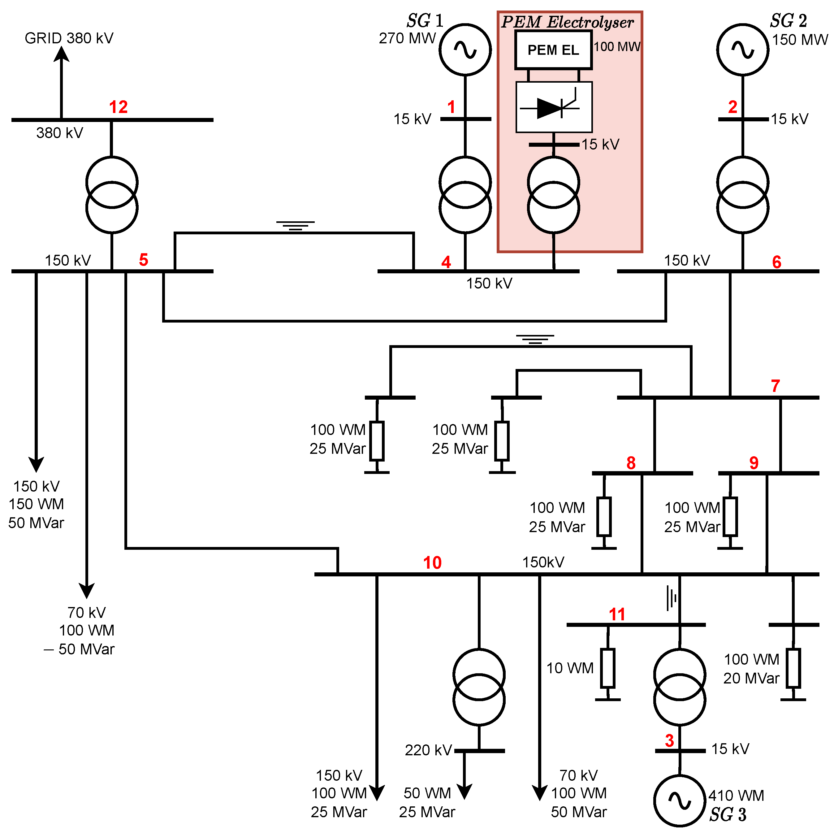
Figure 2.
Dynamic response of the cell voltage of each of the four electrochemical models proposed in the literature as a function of the cell current. The cell input current is set to 5 A.
Figure 2.
Dynamic response of the cell voltage of each of the four electrochemical models proposed in the literature as a function of the cell current. The cell input current is set to 5 A.
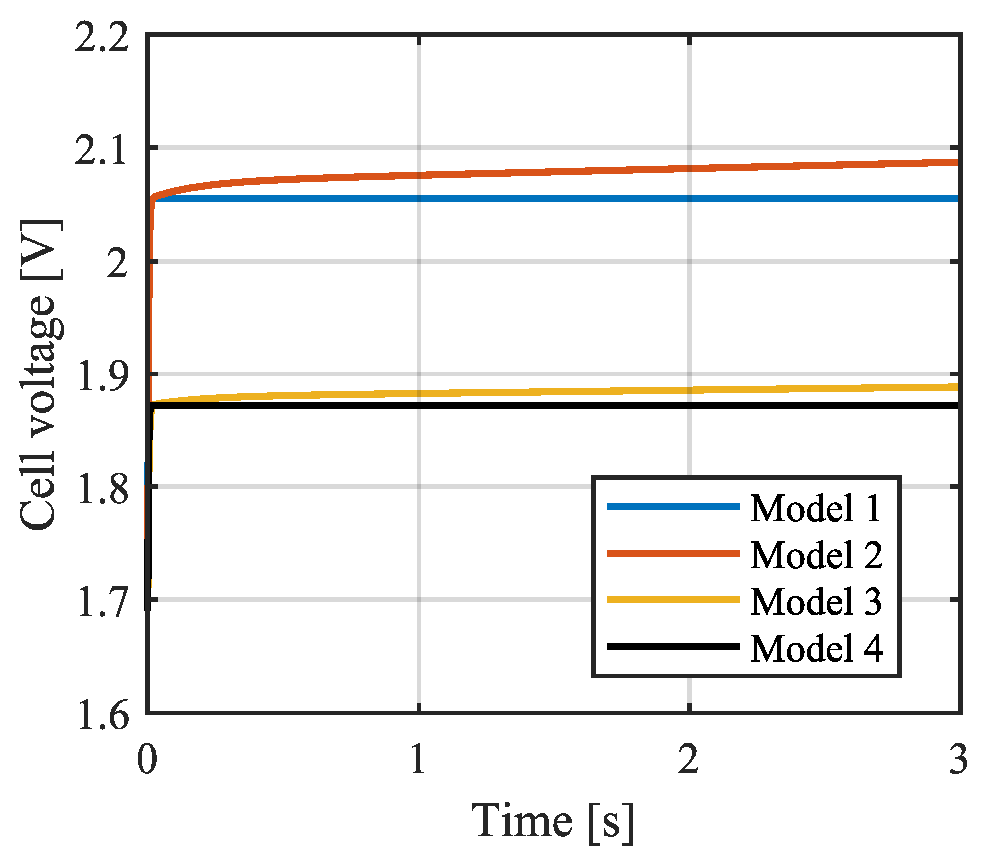
Figure 3.
Transient response of the cell voltage of each of the four electrochemical models proposed in the literature as a function of the cell current. The cell input current is set to 5 A.
Figure 3.
Transient response of the cell voltage of each of the four electrochemical models proposed in the literature as a function of the cell current. The cell input current is set to 5 A.
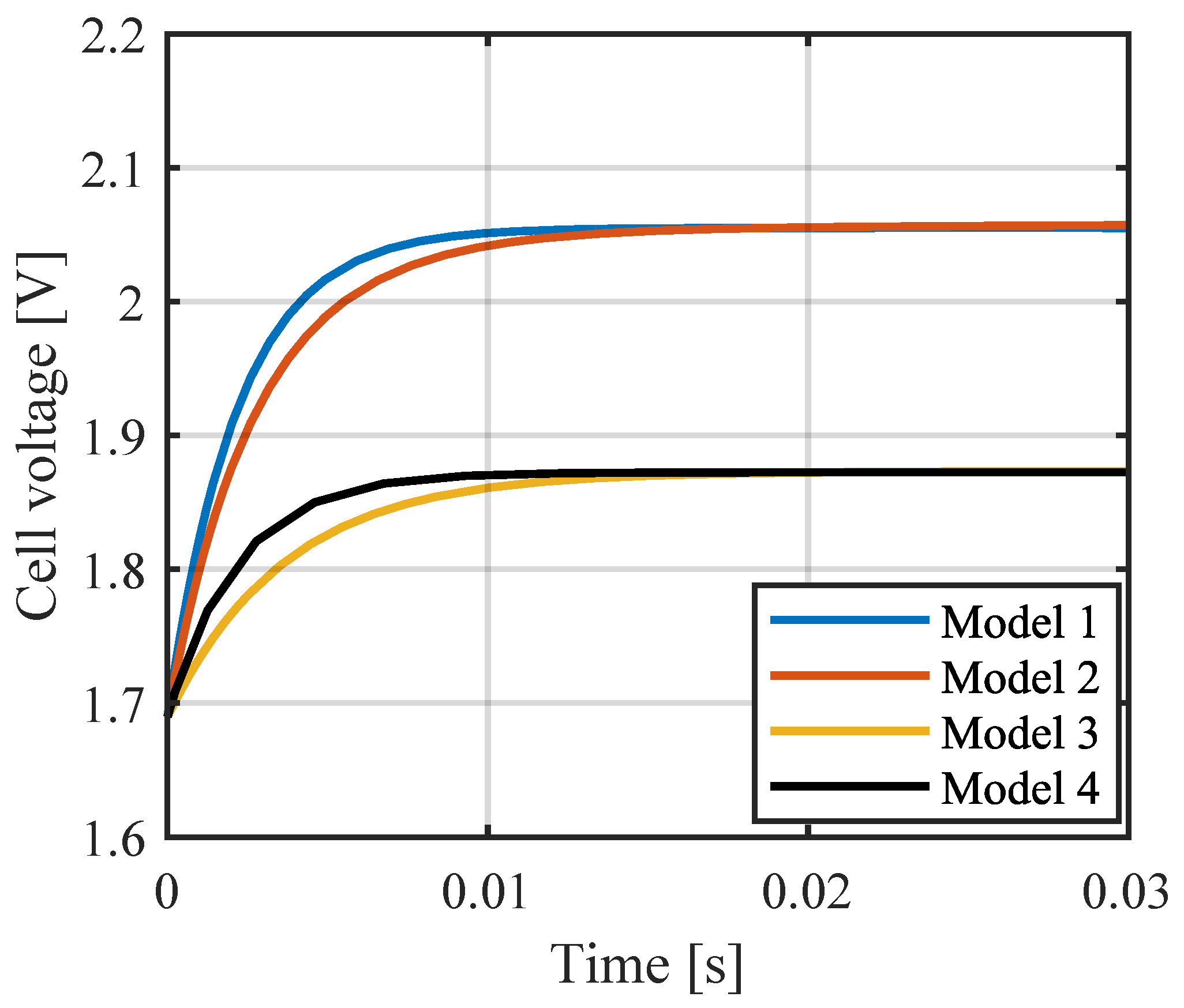
Figure 4.
Hydrogen PEM electrolyser model connected to the grid through a 12-pulse thyristor rectifier.
Figure 4.
Hydrogen PEM electrolyser model connected to the grid through a 12-pulse thyristor rectifier.
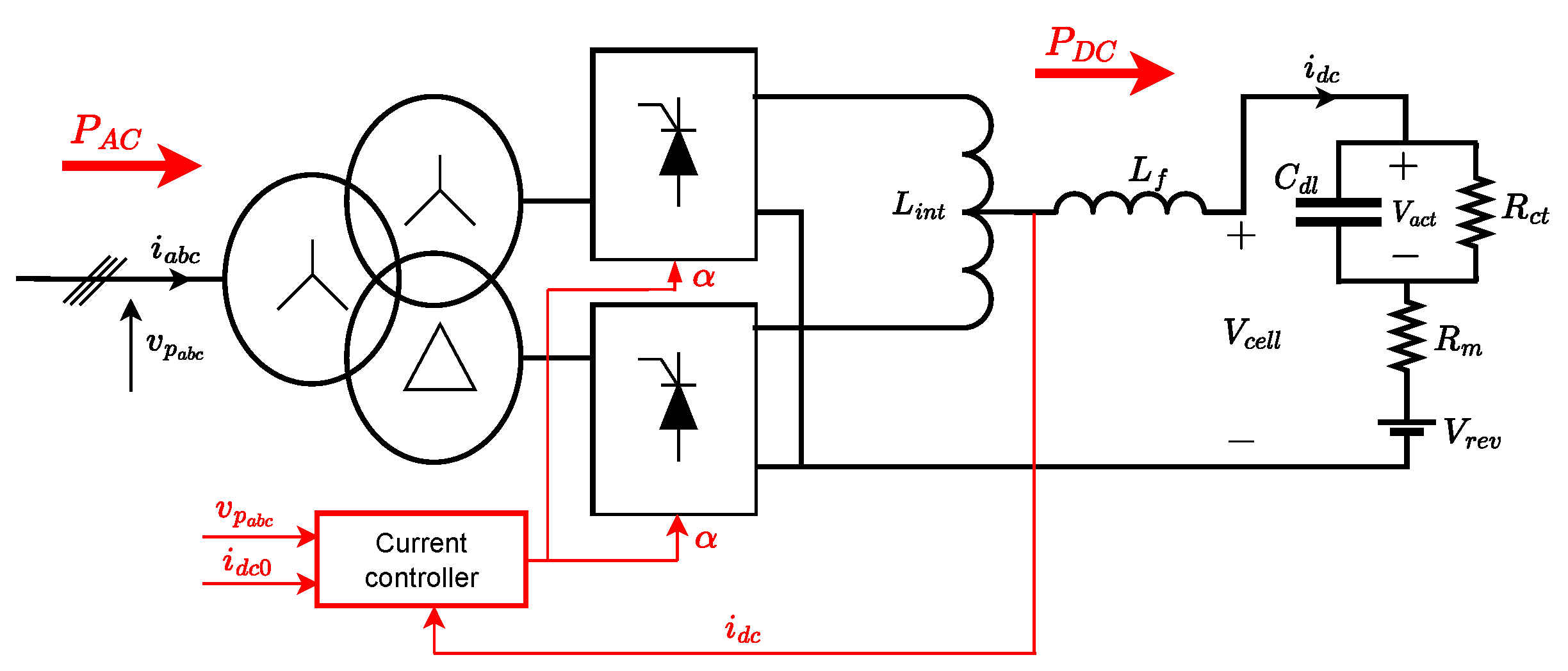
Figure 5.
Electrical model of a PEM electrolyser and 12-pulse thyristor rectifier.

Figure 6.
Physical system of the 12-pulse thyristor rectifier associated with the electrolyser model in the s domain.
Figure 6.
Physical system of the 12-pulse thyristor rectifier associated with the electrolyser model in the s domain.
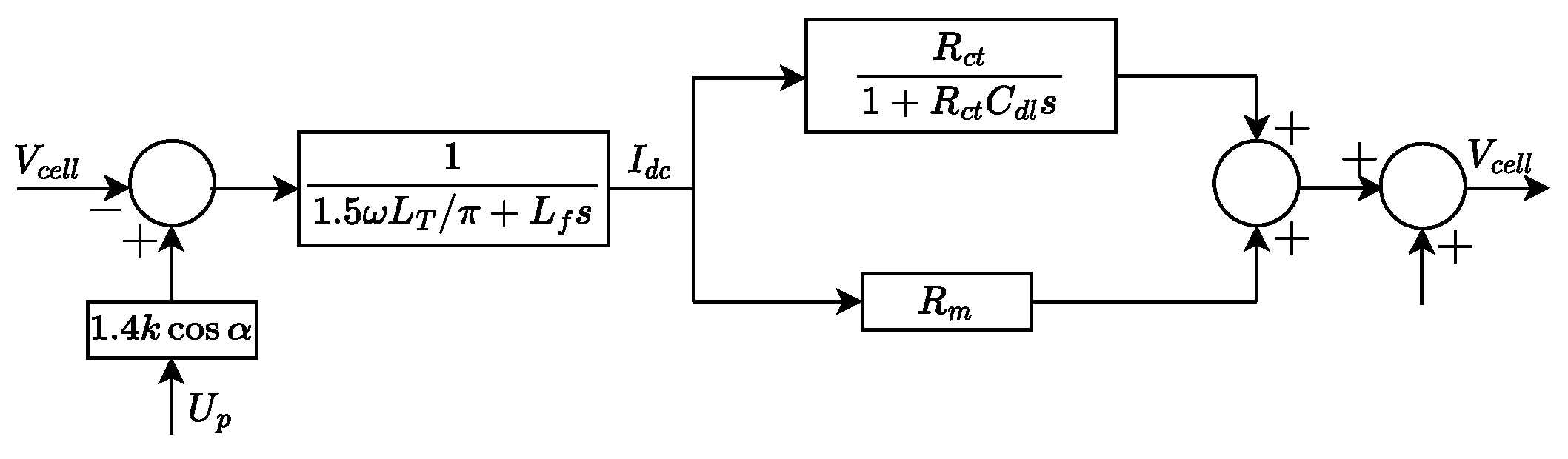
Figure 7.
Complete control structure composed of an internal current control loop and an external voltage control loop.
Figure 7.
Complete control structure composed of an internal current control loop and an external voltage control loop.

Figure 8.
Steady-state conditions of the PEM electrolyser connected to : (a) DC electrolyser current; (b) firing angle; (c) DC voltage.
Figure 8.
Steady-state conditions of the PEM electrolyser connected to : (a) DC electrolyser current; (b) firing angle; (c) DC voltage.
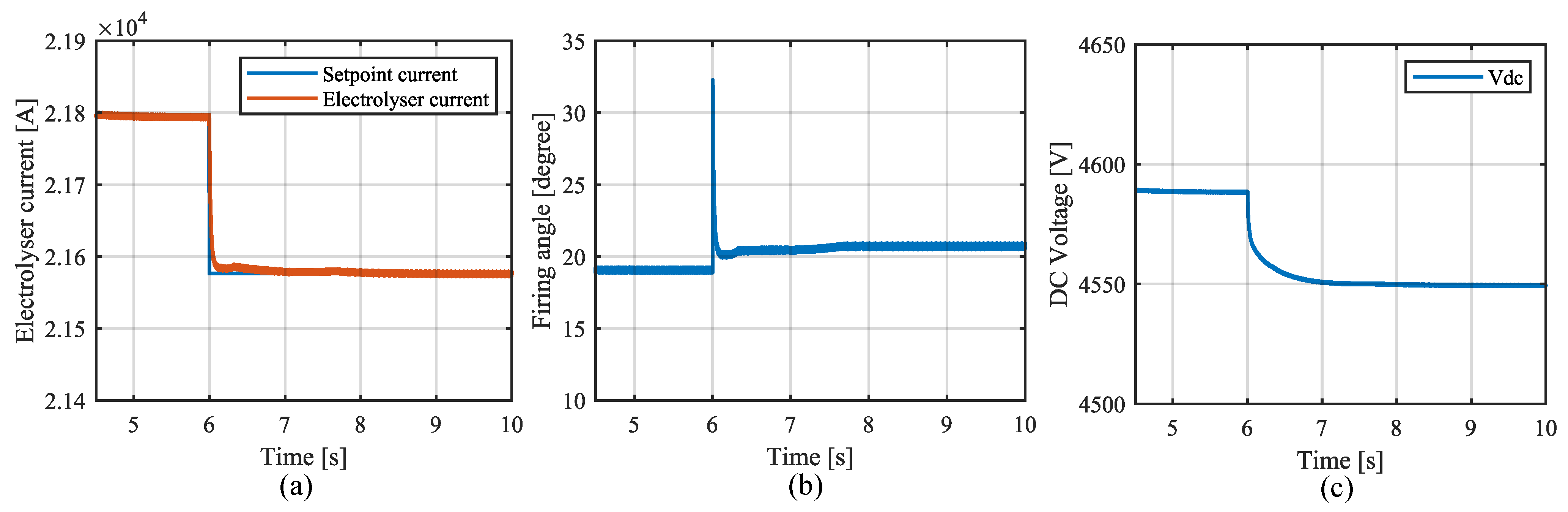
Figure 9.
n PEM electrolyser models connected to the grid through a 12-pulse thyristor rectifier.

Figure 10.
Fractions of constant impedance load and constant current load dependent on the number of electrolysers connected in parallel on the DC rectifier side.
Figure 10.
Fractions of constant impedance load and constant current load dependent on the number of electrolysers connected in parallel on the DC rectifier side.
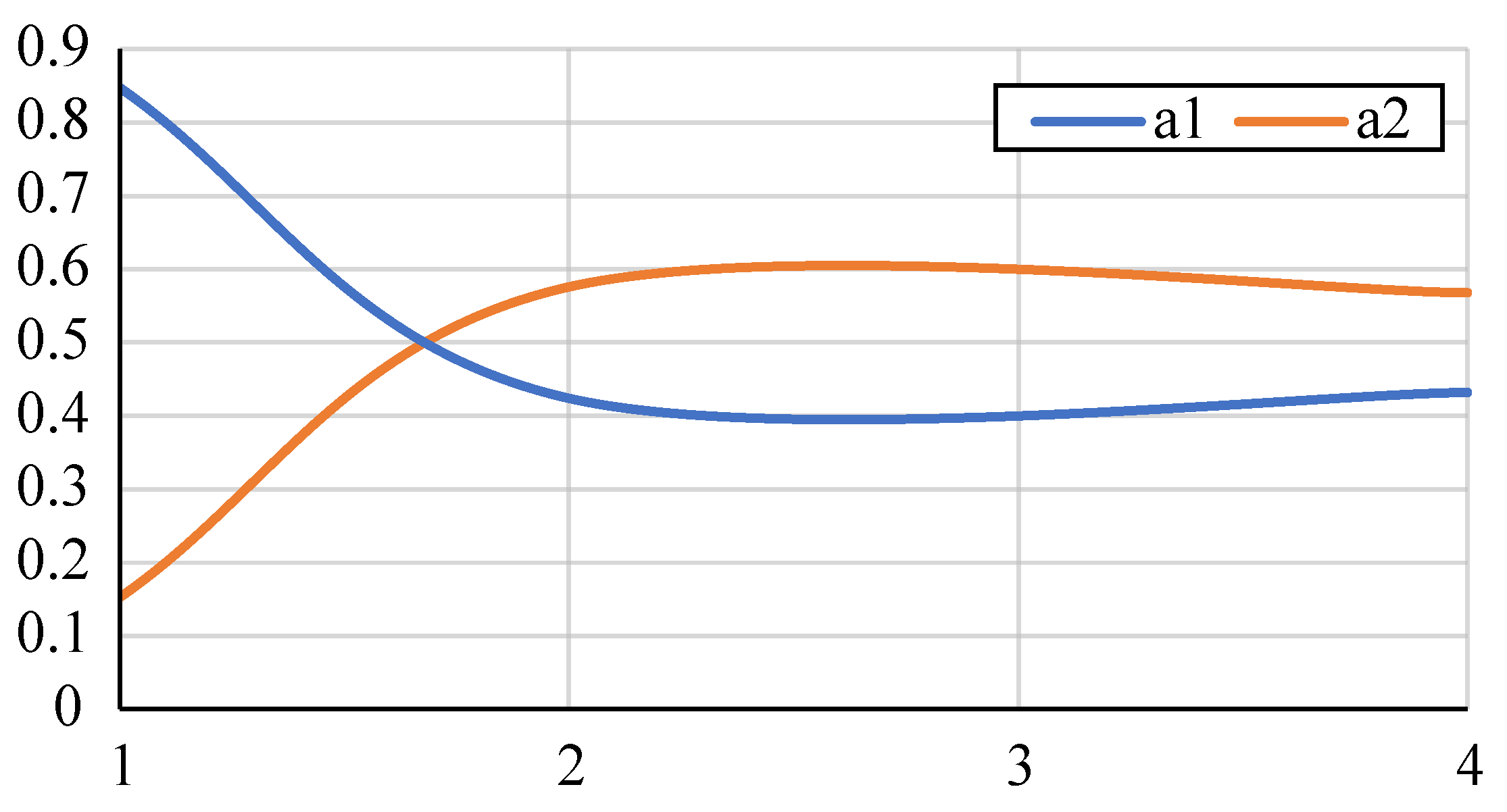
Figure 11.
Firing angle associated with the parameters of the proportional-integral controller.
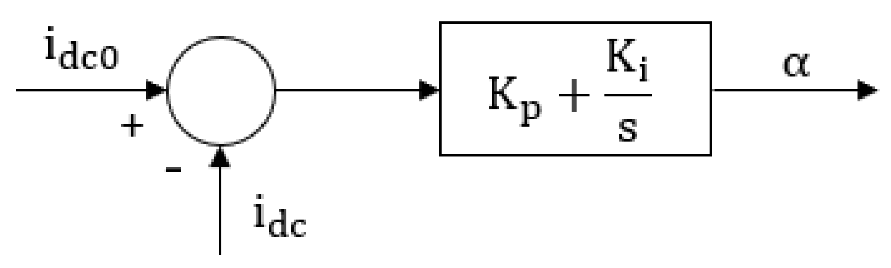
Figure 12.
The modelled system’s modes in the complex plane: (a) without connecting the PEM electrolyser to test system; (b) with 100 MW of PEM electrolysers connected to the grid. The modes in the absence of the electrolyzer are depicted in blue, while those incorporating the electrolyzer are illustrated in red.
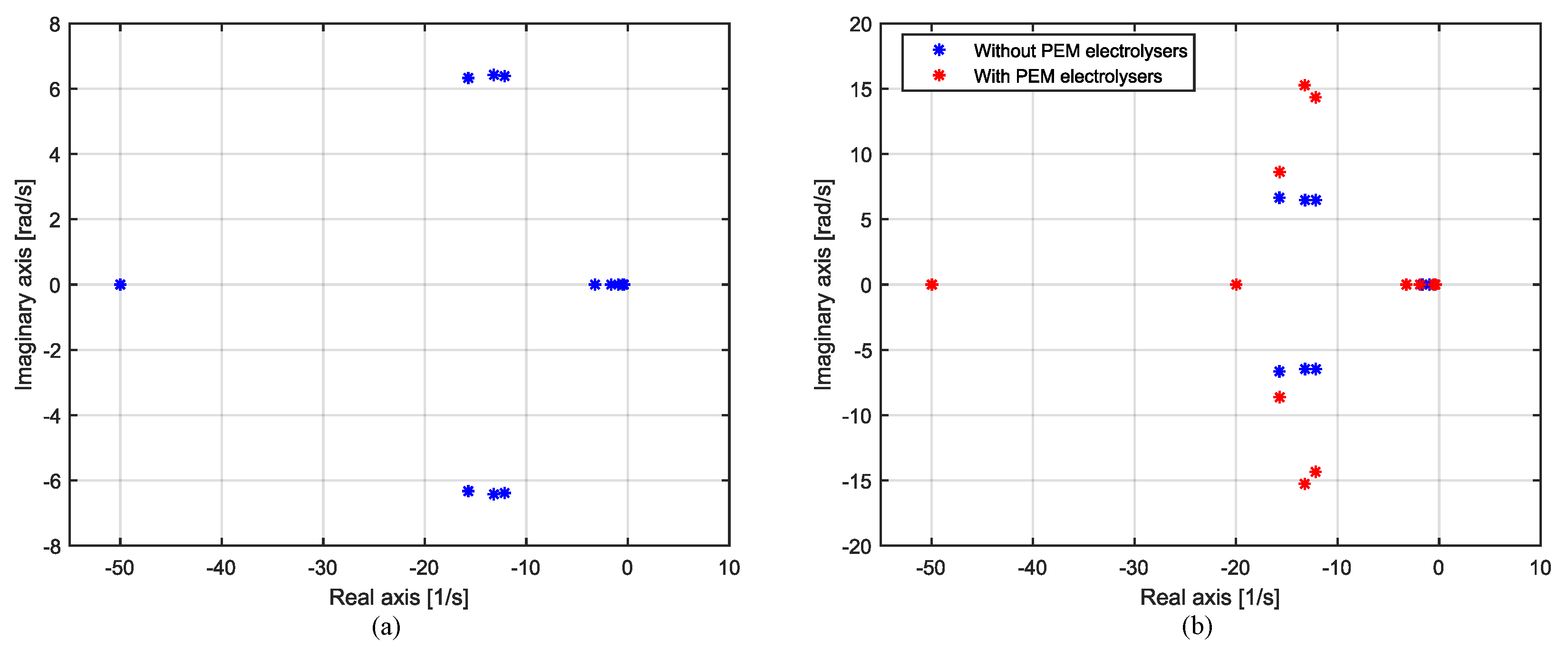
Figure 13.
Movement of modes and caused by changes in the inertial constant value of the synchronous generator connected to : = 3 to 7 s. The modes in the absence of the electrolyzer are depicted in blue, while those incorporating the electrolyzer are illustrated in red.
Figure 13.
Movement of modes and caused by changes in the inertial constant value of the synchronous generator connected to : = 3 to 7 s. The modes in the absence of the electrolyzer are depicted in blue, while those incorporating the electrolyzer are illustrated in red.
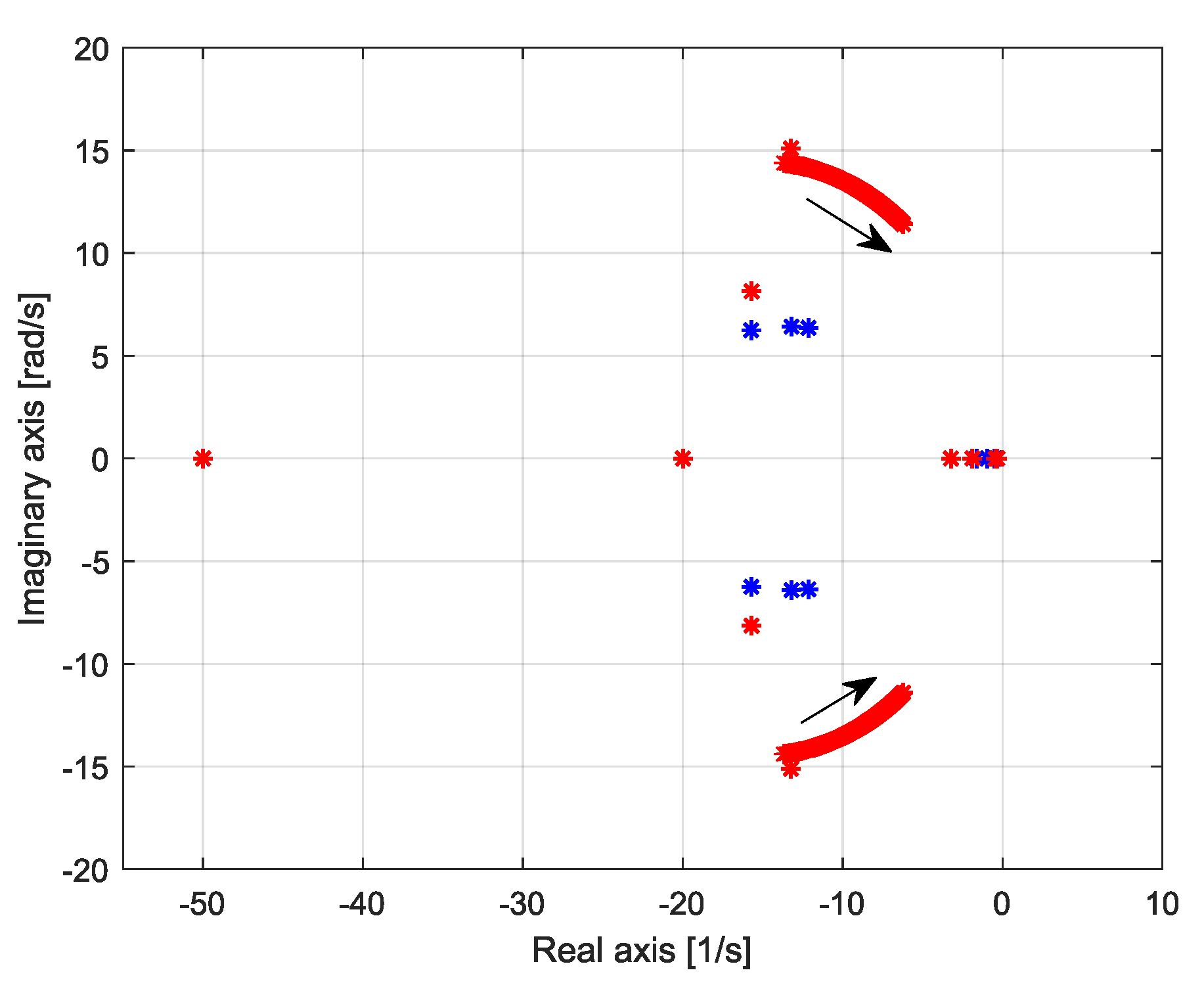
Figure 14.
Movement of- the and modes caused by changes in the inertial constant value of the synchronous generator connected to : = 2.6 to 7 s. The modes in the absence of the electrolyzer are depicted in blue, while those incorporating the electrolyzer are illustrated in red.
Figure 14.
Movement of- the and modes caused by changes in the inertial constant value of the synchronous generator connected to : = 2.6 to 7 s. The modes in the absence of the electrolyzer are depicted in blue, while those incorporating the electrolyzer are illustrated in red.
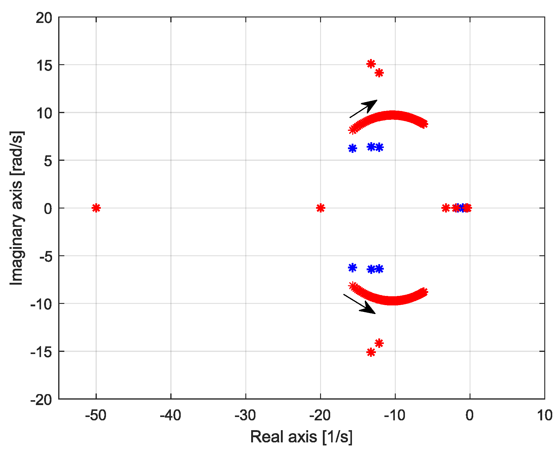
Figure 15.
Movement of the and modes caused by changes in the inertial constant value of the synchronous generator connected to : = 3 to 7 s. The modes in the absence of the electrolyzer are depicted in blue, while those incorporating the electrolyzer are illustrated in red.
Figure 15.
Movement of the and modes caused by changes in the inertial constant value of the synchronous generator connected to : = 3 to 7 s. The modes in the absence of the electrolyzer are depicted in blue, while those incorporating the electrolyzer are illustrated in red.

Figure 16.
Movement of the and modes caused by changes in the damping torque coefficient value of the synchronous generator connected to : = 0.5 to 0.8. The modes in the absence of the electrolyzer are depicted in blue, while those incorporating the electrolyzer are illustrated in red.
Figure 16.
Movement of the and modes caused by changes in the damping torque coefficient value of the synchronous generator connected to : = 0.5 to 0.8. The modes in the absence of the electrolyzer are depicted in blue, while those incorporating the electrolyzer are illustrated in red.

Figure 17.
Movement of the and modes caused by changes in the damping torque coefficient value of the synchronous generator connected to : = 0.5 to 0.8. The modes in the absence of the electrolyzer are depicted in blue, while those incorporating the electrolyzer are illustrated in red.
Figure 17.
Movement of the and modes caused by changes in the damping torque coefficient value of the synchronous generator connected to : = 0.5 to 0.8. The modes in the absence of the electrolyzer are depicted in blue, while those incorporating the electrolyzer are illustrated in red.
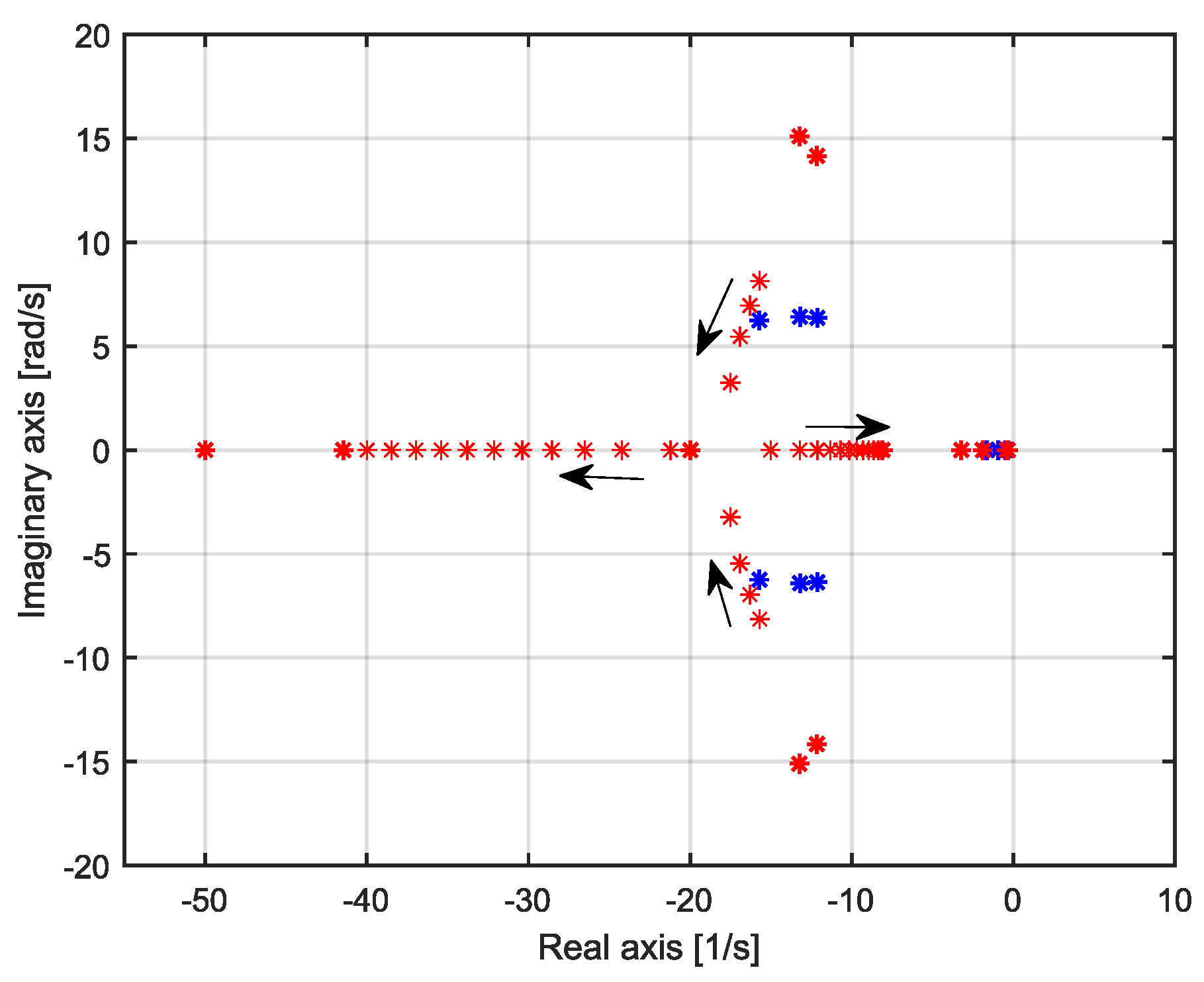
Figure 18.
Movement of the and modes caused by changes in the damping torque coefficient value of a synchronous generator connected to : = 0.5 to 0.8. The modes in the absence of the electrolyzer are depicted in blue, while those incorporating the electrolyzer are illustrated in red.
Figure 18.
Movement of the and modes caused by changes in the damping torque coefficient value of a synchronous generator connected to : = 0.5 to 0.8. The modes in the absence of the electrolyzer are depicted in blue, while those incorporating the electrolyzer are illustrated in red.

Figure 19.
(a) Dynamic response of the rotor speed deviations () and (b) the dynamic response of the rotor angle deviations ().
Figure 19.
(a) Dynamic response of the rotor speed deviations () and (b) the dynamic response of the rotor angle deviations ().
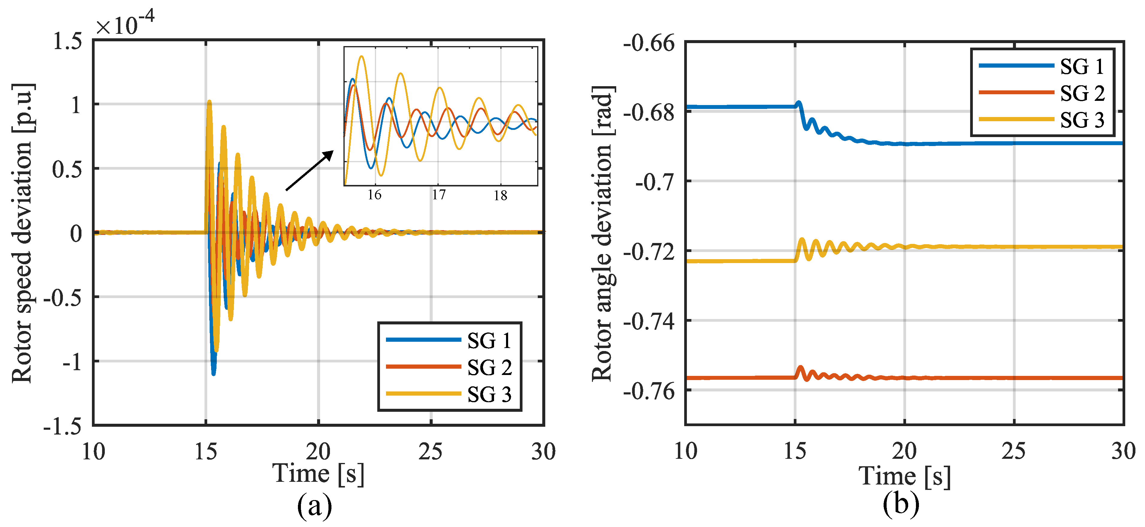
Figure 20.
Dynamic response of electromechanical state variables of when 100 MW of PEM electrolysers are connected to the grid at 15 s: (a) rotor angle deviation and (b) rotor speed deviation with the impact of modelling the electrolyser as a load.
Figure 20.
Dynamic response of electromechanical state variables of when 100 MW of PEM electrolysers are connected to the grid at 15 s: (a) rotor angle deviation and (b) rotor speed deviation with the impact of modelling the electrolyser as a load.

Figure 21.
Dynamic response of electromechanical state variables of when 100 MW of PEM electrolysers are connected to the grid at 15 s: (a) rotor angle deviation and (b) rotor speed deviation with the impact of modelling the electrolyser as a load.
Figure 21.
Dynamic response of electromechanical state variables of when 100 MW of PEM electrolysers are connected to the grid at 15 s: (a) rotor angle deviation and (b) rotor speed deviation with the impact of modelling the electrolyser as a load.
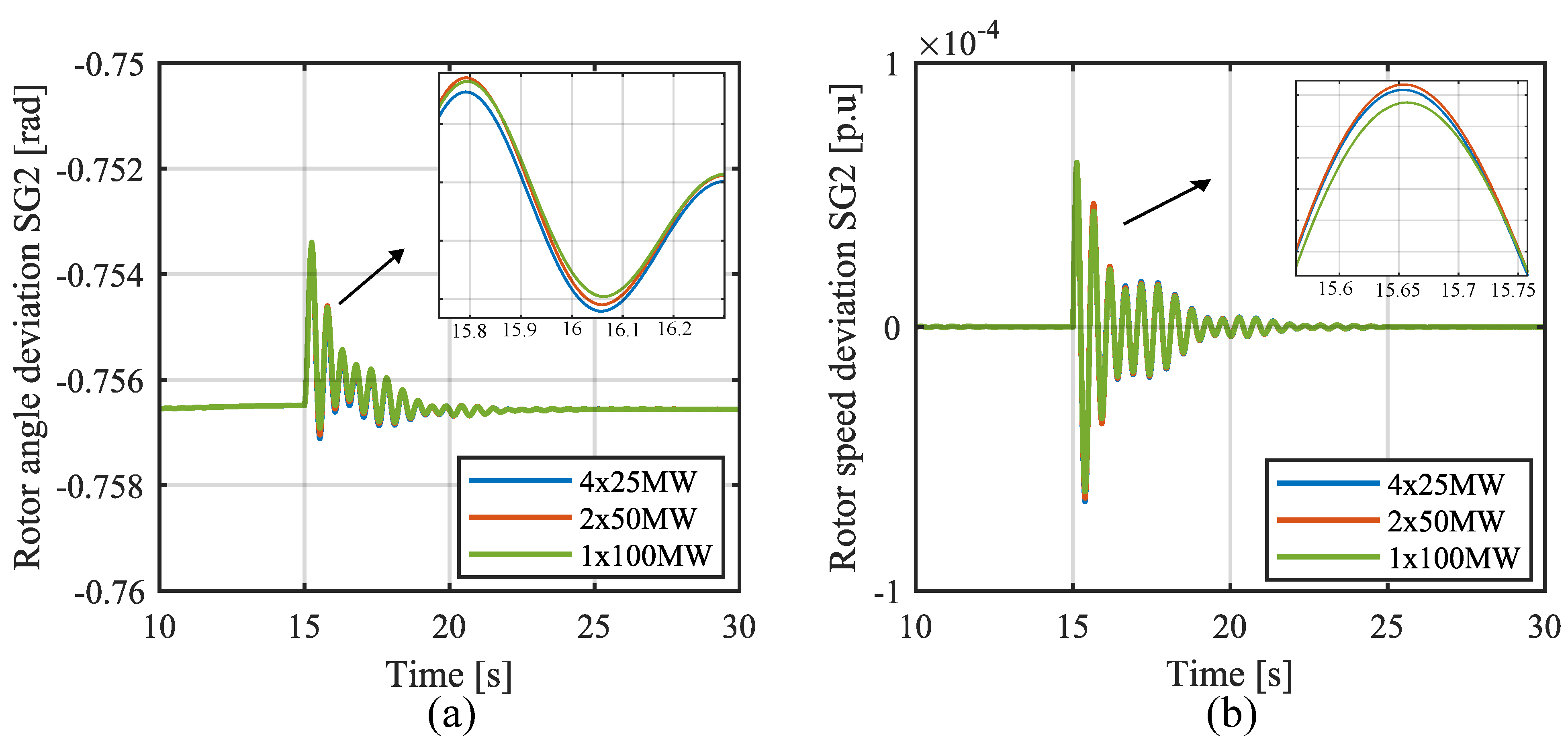
Figure 22.
Dynamic response of electromechanical state variables of when 100 MW of PEM electrolysers are connected to the grid at 15 s: (a) rotor angle deviation and (b) rotor speed deviation with the impact of modelling the electrolyser as a load.
Figure 22.
Dynamic response of electromechanical state variables of when 100 MW of PEM electrolysers are connected to the grid at 15 s: (a) rotor angle deviation and (b) rotor speed deviation with the impact of modelling the electrolyser as a load.
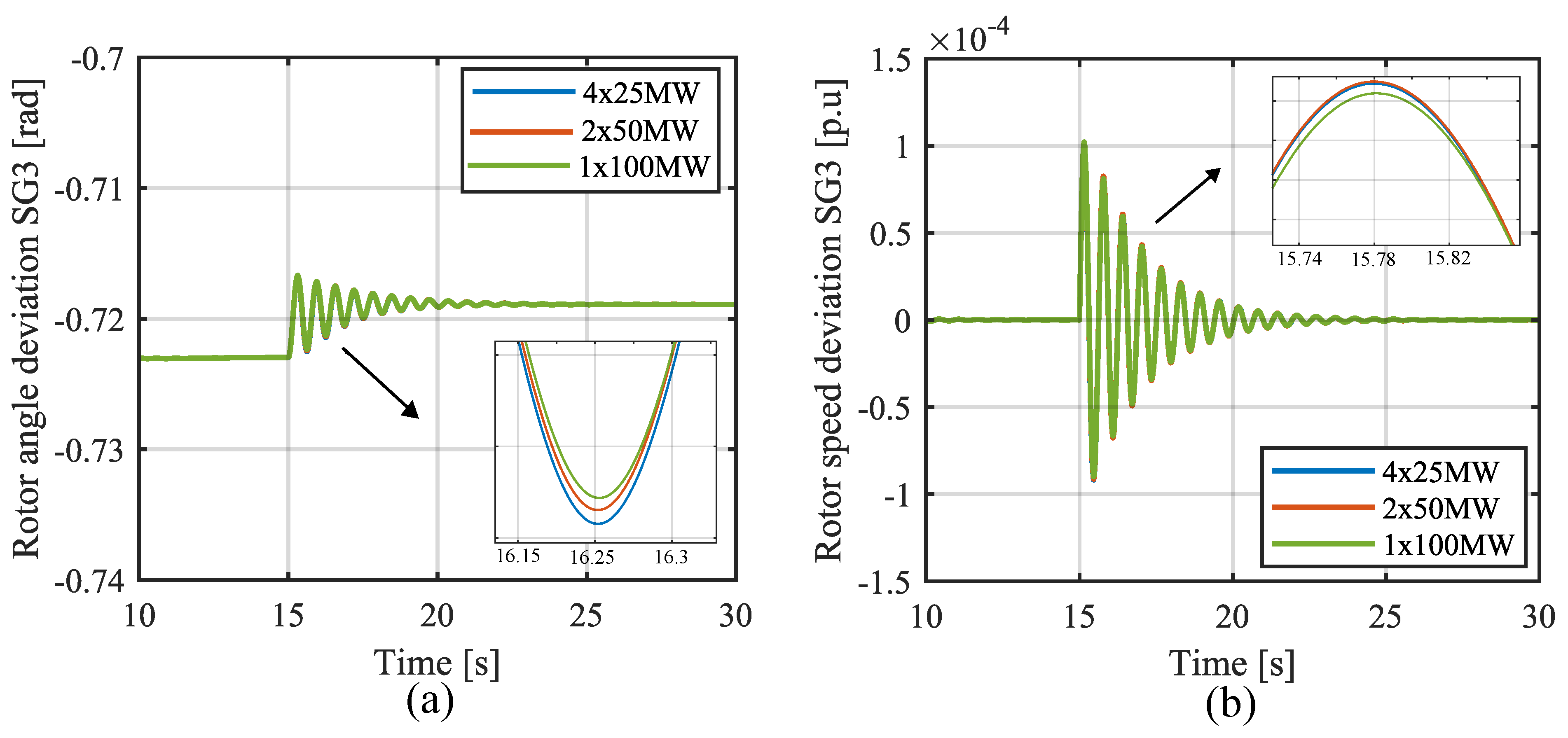
Figure 23.
Dynamic responses of electromechanical state variables of of electrolyser current: (a) DC electrolyser current and (b) rotor speed deviations .
Figure 23.
Dynamic responses of electromechanical state variables of of electrolyser current: (a) DC electrolyser current and (b) rotor speed deviations .


Table 1.
Electrochemical model and PI controller parameters.
| Electrochemical Model | PI Controller |
|---|---|
| R = 0.3818 ; = 0.3318 ; = 0.9091 F; = 700 V; = 48 H | Kp = 0.06; = 0.12; = 40 mH; = 119H; |
Table 2.
Parameter values for test-system components.
| Machine 1 | Machine 2 | Machine 3 |
|---|---|---|
| MW MVar | MW MVar | MW MVar |
| R = 0.089 pu, X = 1.5 pu | R = 0.089 pu, X = 1.5 pu | R = 0.089 pu, X = 1.5 pu |
| X = 0.18 pu, T = 5 s | X = 0.18 pu, T = 5 s | X = 0.18 pu, T = 6 s |
| X = 1.26 pu, T = 0.31 s | X = 1.26 pu, T = 0.31 s | X = 1.26 pu, T = 0.53 s |
| X = 1.26 pu, s | X = 1.26 pu, s | X = 1.26 pu, s |
| Static exciter 1 | Static exciter 2 | Static exciter 3 |
| K = 20, T = 0.02 s | K = 20, T = 0.02 s | K = 20, T = 0.02 s |
| K = 0.063, T = 0.35 s | K = 0.063, T = 0.35 s | K = 0.063, T = 0.35 s |
| K = 1, T = 0.314 s | K = 1, T = 0.314 s | K = 1, T = 0.314 s |
Table 3.
Identification of modes with respect to the state variables of synchronous generators in the case in which the PEM electrolyser is not connected to the test system.
Table 3.
Identification of modes with respect to the state variables of synchronous generators in the case in which the PEM electrolyser is not connected to the test system.
| Mode Values | Identification of Modes |
|---|---|
| , and | |
| , , | |
| , , |
Table 4.
Identification of modes with respect to the state variables of synchronous generators in the case in which 100 MW of PEM electrolysers are connected to the test system ().
Table 4.
Identification of modes with respect to the state variables of synchronous generators in the case in which 100 MW of PEM electrolysers are connected to the test system ().
| Mode Values | Identification of Modes |
|---|---|
| , and | |
| , , | |
| , , | |
Disclaimer/Publisher’s Note: The statements, opinions and data contained in all publications are solely those of the individual author(s) and contributor(s) and not of MDPI and/or the editor(s). MDPI and/or the editor(s) disclaim responsibility for any injury to people or property resulting from any ideas, methods, instructions or products referred to in the content. |
© 2023 by the authors. Licensee MDPI, Basel, Switzerland. This article is an open access article distributed under the terms and conditions of the Creative Commons Attribution (CC BY) license (https://creativecommons.org/licenses/by/4.0/).
Share and Cite
MDPI and ACS Style
Wanlongo Ndiwulu, G.; Vasquez Mayen, E.; De Jaeger, E. Effect of a Large Proton Exchange Membrane Electrolyser on Power System Small-Signal Angular Stability. Electricity 2023, 4, 381-409. https://doi.org/10.3390/electricity4040021
AMA Style
Wanlongo Ndiwulu G, Vasquez Mayen E, De Jaeger E. Effect of a Large Proton Exchange Membrane Electrolyser on Power System Small-Signal Angular Stability. Electricity. 2023; 4(4):381-409. https://doi.org/10.3390/electricity4040021
Chicago/Turabian StyleWanlongo Ndiwulu, Guy, Eduardo Vasquez Mayen, and Emmanuel De Jaeger. 2023. "Effect of a Large Proton Exchange Membrane Electrolyser on Power System Small-Signal Angular Stability" Electricity 4, no. 4: 381-409. https://doi.org/10.3390/electricity4040021