


Stochastic Finite Element Analysis of Root-Reinforcement Effects in Long and Steep Slopes


1
Department of Civil Engineering, Institute of Engineering, Pulchowk Campus, Tribhuvan University, Kathmandu 44601, Nepal
2
Department of Environmental Design, Faculty of CRI, Graduate School of Science and Engineering, Ehime University, Matsuyama 790-8577, Japan
*
Author to whom correspondence should be addressed.
Geotechnics 2023, 3(3), 829-853; https://doi.org/10.3390/geotechnics3030045
Submission received: 8 July 2023
/
Revised: 11 August 2023
/
Accepted: 17 August 2023
/
Published: 23 August 2023
(This article belongs to the Special Issue Recent Advances in Geotechnical Engineering)
Abstract
:This article introduces a novel numerical scheme within the finite element method (FEM) to study soil heterogeneity, specifically focusing on the root–soil matrix in fracture treatments. Material properties, such as Young’s modulus of elasticity, cohesion, and the friction angle, are considered as randomly distributed variables. To address the inherent uncertainty associated with these distributions, a Monte Carlo simulation is employed. By incorporating the uncertainties related to material properties, particularly the root component that contributes to soil heterogeneity, this article provides a reliable estimation of the factor of safety, failure surface, and slope deformation, all of which demonstrate a progressive behavior. The probability distribution curve for the factor of safety (FOS) reveals that an increase in the root area ratio (RAR) results in a narrower range and greater certainty in the population mean, indicating reduced material variation. Moreover, as the slope angle increases, the sample mean falls within a wider range of the probability density curve, indicating an enhanced level of material heterogeneity. This heterogeneity amplifies the level of uncertainty when predicting the factor of safety, highlighting the crucial importance of accurate information regarding heterogeneity to enhancing prediction accuracy.
1. Introduction
Slope stability problems inherently involve uncertainty and variability due to the natural composition of slopes, which exhibit heterogeneity. The soil properties within these slopes exhibit variations in both the vertical and horizontal directions. Deterministic approaches provide straightforward solutions based on known relationships between input parameters, disregarding random variables and the associated uncertainty. However, such approaches fail to capture the inherent uncertainty linked to material properties, often resulting in conservative outcomes. A review of input uncertainty research in stochastic simulations was conducted by Canan et al. [1], covering classification, recent developments, and real-world applications. Likewise, sources of uncertainty in site characterization and their impact on geotechnical reliability-based design are discussed by Aladejare et al. [2]. In slope stability analysis, probabilistic or stochastic methods have emerged as valuable tools for addressing the complexities of uncertain soil behavior. Researchers have explored the stochastic finite element method [3], considered progressive failure [4], and developed new approaches to risk modeling [5,6]. Additionally, they have examined the influence of soil behavior on slope stability using finite element analysis [7,8,9]. These studies collectively demonstrate the value of probabilistic and stochastic methods in understanding slope stability under uncertain conditions, offering insights for future research and practical applications.
To address varying degrees of uncertainty, a simplified approach is typically used, but it may not fully account for material heterogeneity. In cases where material heterogeneity significantly impacts the study, a stochastic approach is preferred. Researchers have extensively investigated the spatial variability of soil parameters in slope stability analysis (e.g., [10,11,12,13,14,15,16]). The stochastic process has proven to be an effective tool for capturing the spatial variability of soil properties in natural soil slopes. Previous studies have employed random theory to generate property distributions within finite elements and examine the influence of soil heterogeneity on slope stability [17,18,19,20]. Finite element analysis has also been utilized to assess the impact of heterogeneity on the stability of clay slopes, particularly in terms of spatially varying undrained shear strength [21]. Additionally, studies have explored the probability of failure in cohesive slopes using both simple and advanced probabilistic methods [13].
The conventional approach to slope instability analysis compares “disruptive forces” to “restorative forces” through the factor of safety (FOS). Deterministic methods such as finite element analysis overlook soil variability and heterogeneity. To address this issue, our study introduces a new numerical scheme using stochastic processes to capture uncertainties in physical quantities. Material properties (e.g., Young’s modulus, cohesion, and the angle of internal friction) are treated as randomly distributed variables. Monte Carlo simulation generates probability distribution functions for the response, allowing for the exploration of material heterogeneity. This comprehensive approach enhances slope stability assessments by considering the probabilistic nature of material properties, enabling more informed decisions in geotechnical engineering.
This study evaluates the applicability of a stochastic process in assessing the impact of root reinforcement on slope stability. The primary objective is to determine the probability of failure in soil slopes, particularly in cases where our understanding of material properties and spatial distribution is limited, making deterministic analysis inadequate. To address this challenge, we employed a Monte Carlo method for stochastic finite element analysis, which was specifically designed to handle the heterogeneous behavior of soil materials in slope stability problems.
Additionally, we utilized a novel numerical scheme in fracture treatment for stochastic finite element computation. This approach enabled us to accurately determine the progressive failure surface and corresponding factor of safety. The Monte Carlo method efficiently solved the stochastic problem by utilizing a computer program with a pseudo-random number generator, generating diverse attribute values within the system. The resulting statistical measures were then visualized using appropriate tools, providing a comprehensive understanding of the outcomes.
Moreover, this research facilitates the clear interpretation of the findings through probability density functions (pdf) and cumulative distribution functions (cdf). These analytical tools significantly enhance our understanding of the statistical characteristics exhibited by the system. By employing a rigorous stochastic analysis framework, this study contributes to a more comprehensive assessment of slope stability and assists in making informed decisions in geotechnical engineering projects.
2. Materials and Methods
2.1. Mathematical Formulation
In this study, a novel formulation is employed to investigate the complex behavior of soil–root interactions. This innovative approach combines the fundamental principles of the Finite Element Method (FEM) with a robust formulation capable of accurately handling the abrupt transition from a continuous displacement function to a discontinuous displacement function. The resulting finite element equation is expressed as follows [22]:
where:
and:
This formulation incorporates the mass matrix , stiffness matrix , and force matrix , which are integral components of the analysis. The symbols are used for the index notations. The system under consideration is in a dynamic state, subject to body forces in the traction and displacements on . The formulation follows indicial notation and the summation convention, where indices such as and range run from 1 to 2 in a two-dimensional case. The comma (,) denotes partial derivatives of variables with respect to the corresponding index.
The boundary of the domain evolves over time as fractures propagate. This dynamic boundary can be either traction-free or subject to specified traction conditions. To account for the influence of root reinforcement, we introduce an average elasticity tensor for linearly elastic isotropic materials and an average mass density into the mathematical formulation. These additions enable a comprehensive analysis of the root-reinforcement effect:
where and are known, respectively, as the weight function of the roots, the weight function of the soil, the density of the roots, the density of the soils, and the root area ratio (RAR). In order to thoroughly explore the impact of vegetation on slope stability, we conducted an extensive review of the relevant literature [23,24,25,26,27,28]. To provide a visual representation of the computational process employed in this study, we present Figure 1, which illustrates the key aspects of the FEM. The Lagrange interpolation function is utilized as the interpolation scheme, while the integration of the domain’s response, encompassing the displacement and stress fields, is performed using the Gauss–Legendre (GL) method. The integration of stochastic methods within FEM introduces randomness into the analysis, leading to probabilistic outcomes. This allows us to assess the probability of slope failure and estimate the uncertainties associated with the computed results. By combining FEM with the stochastic method, we gain valuable insights into the potential range of slope stability outcomes and obtain more robust and realistic estimations of the system’s behavior under uncertain conditions. This combined approach enables a comprehensive analysis of the domain and facilitates a deeper understanding of the influence of vegetation on the stability of slopes. While Figure 1 illustrates the general FEM used in this study, we later present a separate figure for the stochastic FEM.
We suppose that denotes the probability density distribution of certain characteristic data, expressed as follows:
Density functions can be interpreted as probabilities. If we denote the probability density function as , we have the following expression:
If we consider a density function, denoted by , representing a specific quantity, the cumulative distribution function for this quantity can be defined as follows:
The probability density function represents a smoothed version of a histogram, providing a compact form that facilitates integration for probability calculations. Among the various probability distributions, the normal distribution is widely adopted due to its suitability for approximating a large number of independent random variables. This distribution exhibits symmetry around the mean value. The probability of a given range can be determined by evaluating the area under the bell-shaped curve, as depicted in Figure 2. Notably, the total area under the curve ( to ), spanning from negative infinity to positive infinity, is equal to unity. In a normal distribution, the probability density function is characterized by a mean value (μ) and a standard deviation (σ). It describes the likelihood of obtaining a particular value within the distribution. The reveals that the highest probability is concentrated around the mean, while the probabilities decrease towards the tails of the distribution. The mathematical expression for the probability density function of a normal distribution with mean and standard deviation is as follows:
Cumulative probability is the total probability in the range to , as shown in Figure 2, and it can be represented by the normal distribution curve as follows (Equation (7)):
Monte Carlo simulation is one of the most commonly employed numerical methods. This approach utilizes pseudo-random numbers, , that are uniformly distributed over a given interval . It is essential that the generated random numbers are independent and do not exhibit any correlation with each other. The Monte Carlo simulation involves introducing a stochastic equation to carry out the simulation process:
In this equation, the stochastic variable, the mean of the stochastic variable, and the random number with the desired distribution characteristics (having an average of zero) are denoted as and , respectively. This study focuses on a random trial process aimed at establishing a probability distribution function. The Monte Carlo method involves first identifying all variables and then determining the probability distributions for each independent variable. During each trial, a random value is selected from the distribution function and used in the computation. The ultimate outcome of a Monte Carlo simulation is a probability distribution of the parameter.
Past researchers have extensively investigated stochastic soil modeling. Discussions have included the utilization of the stochastic FEM with a first-order approximation. It has been observed that soil heterogeneity not only introduces variability in the computed response but also affects the failure mechanism [29]. The Monte Carlo method has been employed to address soil variability in the limit equilibrium method (LEM) [30]. Additionally, extending the traditional LEM of slices to a probabilistic approach enables the assessment of spatial variation in soil strength parameters [31]. Random FEM has also been employed to capture soil variability [32]. The literature provides an overview of soil heterogeneity [33], with a specific focus on spatial variability in soil stiffness and strength [34]. The significance of soil variability in factor of safety calculations has been emphasized [35], highlighting the influence of soil hydraulic properties on soil heterogeneity [36]. In the context of landslide hazard mapping, researchers have used Monte Carlo simulation to study the case of Taiwan [37]. Furthermore, a Monte Carlo simulation approach has been proposed for the spatial probabilistic modeling of slope failure [38]. In this specific formulation, the strength reduction technique has been implemented to initiate and propagate failure [39,40,41,42]. At the end of the research work, the validation process entails conducting a thorough examination and comparing the simulation results with those obtained using other established techniques and tools. This crucial step aims to ensure the accuracy and reliability of the model, confirming its ability to faithfully represent the actual behavior of the system under study.
2.2. Modelling Domain and Progressive Fracture
The FEM is a computational technique used for analyzing the stress–strain behavior of structures. In FEM, the domain is divided into smaller elements, often represented by Delaunay tessellations, as depicted in Figure 3a. This discretization allows us to study the progressive nature of the failure surface. In FEM, the domain is discretized into smaller elements using Delaunay tessellations, enabling the study of the progressive nature of the failure surface because each element’s behavior can be individually analyzed and tracked as the load is applied, allowing for a detailed understanding of failure mechanisms and deformation patterns. By implementing a variable rate of shear strength mobilization at each point on the failure surface, as shown in Figure 3b, we can simulate the phenomenon of progressive failure. This enables the computation of the progressive FOS at every point (A, B, C…) on the failure surface. A stress–strain diagram for progressive failure is presented in Figure 3c. To account for material heterogeneity, variations in soil properties are introduced, as shown in Figure 3d. It provides heterogeneous soil material properties with upper and lower bounds, represented by a color legend. A clear visual representation of the variations in soil properties will be helpful for understanding the level of uncertainty in the material model and how it impacts the analysis or simulation results. This numerical scheme enables the prediction of potential failure zones and the determination of deformation and stress levels within the analyzed domain. However, accurately calculating the precise failure path or surface is a complex task that requires further analysis and computation.
To establish a reliable numerical model capable of capturing the progressive failure behavior in heterogeneous soil slopes, it is crucial to integrate a robust analytical approach for fracture treatment. Through adaptations to the conventional FEM, we can effectively evaluate critical factors such as the FOS, the influence of heterogeneity and variability on slope behavior, deformation patterns, and the implications of uncertain material properties.
Figure 4a presents a diagrammatic representation of the evolution of the domain boundary in this modeling approach. The fracture path is assumed to pass along the element edges, eliminating the need for re-meshing. This maintains the same level of discretization as FEM and ensures ease of use in terms of the discretization function (Figure 4b). To address the computational challenges associated with the interpolation and integration points located at different positions, we implemented three distinct fracture treatment cases in our method for modeling progressive slope failure. In the first case, when failure is initiated at the boundary element of the domain, we introduce an additional node and an extra element. Similarly, in the second case, when failure originates within the domain, we introduce two extra nodes and two additional elements. This adjustment ensures equilibrium within the system while considering the progressive failure phenomenon. Lastly, in the third case, when failure occurs near the domain boundary, we introduce one extra node and two additional elements to accurately capture the behavior of the failure process. These modifications enhance the robustness of our numerical model for heterogeneous soil slopes, allowing us to simulate progressive failure with greater accuracy and efficiency. Further details and discussions regarding this technique can be found in the existing literature [22].
In this study, we successfully adopted the same methodology used in the deterministic approach to incorporate a stochastic approach. This innovative technique, utilizing the Mohr–Coulomb failure criteria and the fundamental principles of fracture mechanics, allows us to assess the influence of root reinforcement on the stability of soil slopes within the framework of the FEM. In this article, we presented a modeling approach that combines FEM with fracture mechanics principles to accurately simulate progressive slope failure. This method considers failure initiation, propagation, and boundary effects using additional nodes and elements for improved accuracy.
To assess the impact of vegetation on slope stability, we developed a comprehensive technique that incorporates various vegetation-related parameters. This approach involves discretizing the domain into both coarser and finer meshes, allowing us to distinguish the root zone effectively. The finer meshes specifically represent the areas where roots are present, and their properties are defined using a homogenization approach. This enables us to accurately account for above-surface and below-surface vegetation-related parameters within the problem domain. The above-surface portion of the vegetation is treated as a traction boundary, encompassing factors such as the wind load, vegetation weight, and structural load. On the other hand, the below-surface part of the vegetation is directly integrated into each finite element as material properties. This inclusive approach enables us to consider the specific characteristics of the vegetation in our analysis. To simulate real-world scenarios of slope instability in two-dimensional cases, we applied fixed boundaries at the bottom and vertical movable boundaries on the left and right sides of the domain. This boundary configuration effectively reflects the practical conditions observed in the field.
2.3. Model Material Properties
In this study, we employed a soil material model that aligns with the Unified Soil Classification System (USCS) [43,44] and has the basic properties shown in Table 1.
In this analysis, we incorporated various elasto-plastic parameters to characterize the soil behavior. The soil-related parameters include an elastic modulus, a Poisson’s ratio of 0.30, and a dilation angle of 0 degrees [11,12,13,14]. These values align with commonly accepted practices in soil bio-engineering modeling. For root-related parameters, we consider the elastic modulus of the roots and the mean tensile strength of the roots. In our model, we assume an elastic modulus within a specified range, and a mean tensile strength of 40 kN/m². It is important to note that the actual tensile strength of roots depends on their diameter, which can range between 5 and 40 kN/m² for different vegetation species. While we have not included the enhanced effective soil cohesion due to evapo-transpiration or the friction of roots in this analysis, we acknowledge their potential influence on slope stability [27,28]. Our program, however, allows for the incorporation of these parameters in future studies. Additionally, we consider a root area ratio ranging from 0.1 to 1.0% and a root zone depth of 2.0 m, representing mature vegetation. While our analysis does not account for the effects of the vegetation load, wind load, soil arching, and buttressing, our program has the capability to incorporate these factors. The focus of this paper primarily centers on root-related parameters, which play a dominant role in evaluating the effectiveness of vegetation in reinforcing slope stability.
To determine Young’s modulus of elasticity and Poisson’s ratio, we can refer to several published works [45,46,47,48,49,50]. As a general guideline, we suggest using an average value of Young’s modulus ranging from X to Y for different soil types within the USCS. For example, ‘clean gravel’ with a well-graded composition (GW) can have a suggested value of of , while clayey gravel with a high content of fine plastics (GC-CH) can have a suggested value of . The values and can vary for the remaining soil types, ranging from silty sand with many fine grains (SM-ML) to inorganic silt with high-compressibility elastic silt (MH). Similarly, the Poisson’s ratio can be employed based on the soil type. For the first and second categories of soil, a suggested value of 0.25 can be used, while, for the third category, a value of 0.3 is recommended. The fourth category can have a Poisson’s ratio of 0.325. These values provide a theoretical framework for modeling and offer insights into the potential slope instability associated with different slope geometries and material models utilizing USCS soils. They also facilitate a preliminary estimation of slope geometry and material properties. However, it is important to note that this method is applicable only to shallow-seated failures. Deep-seated failures require detailed information on soil stratifications and groundwater profiles, which necessitate a separate slope instability analysis.
In our numerical analysis of slope stability, we employed a widely used pseudo-random number generator to introduce variability into the parameters. The generator produces random values that are uniformly distributed between 0 and 1. We varied cohesion (kN/m2) and friction (degrees) within ±10 and ±4, respectively, at an interval of 1, the slope angle from 20 to 50 degrees at an interval of 5, and the root area ratio from 0.6% to 0.9% at an interval of 0.1. The seed value was set to 12,345, ensuring consistency in the subsequent simulations. This approach allows us to accurately and efficiently explore the impact of different parameter combinations on slope stability.
2.4. Numerical Techniques
Figure 5 showcases a simplified flow chart depicting the calculation process for assessing the fracture response in heterogeneous soil slope conditions. We utilized our in-house-developed FEM program to implement the proposed model and perform the calculations illustrated in Figure 5. This program was specifically designed to handle the stochastic analysis and incorporate the root–soil fracture mechanics. The stochastic approach is employed across seven distinct soil slope models, encompassing a range of incline angles. The slope angles considered in this study include 20, 25, 30, 35, 40, 45, and 50 degrees, spanning from mild to steep slopes. These models utilize a common soil material model based on the USCS soil classification system shown in Table 1, along with specific root-related parameters. It is widely recognized that natural soil deposits exhibit inherent variability even within a single soil layer, and even in cases where the deposit appears relatively homogeneous. This variability is attributed to the complex geological formation process and the history of the soil. In probabilistic analysis, standard deviation values are used to account for soil variability. The standard deviation provides a straightforward measure of the uncertainty related to multiple factors, such as soil sampling, soil testing, and measurement errors. A small standard deviation suggests that the dataset is closely grouped around the mean, whereas a large standard deviation indicates a notable dispersion or variability from the mean.
3. Theoretical Verification of the Model
To validate our stochastic findings, we conducted a comparative analysis using the open-source program Specfem3d-Geotech, which is based on the spectral element method [51]. Specifically, we compared the computational results obtained from our stochastic approach to those obtained using Specfem3d-Geotech for a 30-degree slope with a slope length of 200 m and a soil depth of 10 m. In our analysis, we utilized the USCS clay soil (CH) as the material model. Although Specfem3d-Geotech is a 3D spectral element method program, we appropriately configured the boundary conditions to create a plain strain problem, effectively equivalent to 2D modeling. The result obtained using this numerical scheme in one of the computations indicates a FOS of 1.4 with a 75% probability. This value aligns reasonably well (FOS: 1.35) with the spectral element computation, which employed a spectral element budget of 10,000, a spectral degree of 3 orders, a nonlinear iteration of 5000, and a nonlinear tolerance of 0.0005. It is worth noting that some discrepancies may exist in the results, which can be attributed to the stochastic interpretation method employed in our findings.
Tool verification is crucial to ensuring the accuracy and reliability of our program based on the FEM. By conducting a comparative analysis with a higher-order FEM tool such as Specfem3d-Geotech, which employs the spectral element method (SEM), we validated our program’s results against a more sophisticated and advanced tool. This verification process helps to establish the credibility of our methodology and provides confidence in the computational findings. We included validation with the existing literature but not with in situ measurements. The validation of our program with reference to the literature, along with the comparison with another open-source program, demonstrated the effectiveness and reliability of our proposed stochastic modeling approach [12].
Our research outputs are unique, and we focused on the development and validation of tools and techniques rather than replicating existing results. The comparison highlights the novelty and contributions of our proposed stochastic finite element method, which allows for a more comprehensive assessment of slope stability, accounting for the effects of root reinforcement and uncertainties. In addition, the results we produced align well with the general understanding of slope stability with root reinforcement. Our findings provide valuable insights into the influence of the root area ratio and other soil-related parameters on slope stability, corroborating and enhancing the existing knowledge in the field.
4. Results and Discussion
The focus of this study primarily revolves around two key aspects, progressive failure and the progressive factor of safety, while also considering the impact of material variability on the factor of safety. Progressive failure refers to the gradual development and propagation of failure mechanisms within the slope, leading to potential instability. This phenomenon is of significant interest in slope stability analysis as it allows for a more comprehensive understanding of the failure process.
The progressive factor of safety is a measure used to assess the stability of the slope at different stages of failure. It takes into account the changing conditions and the evolving failure mechanisms, providing insights into the safety margin throughout the progression of failure. Additionally, this study examines the influence of material variability on the factor of safety. Soil properties, such as strength and stiffness, are known to exhibit inherent variability due to factors such as geological processes and soil history. By considering this material variability, a more realistic assessment of slope stability can be achieved. Overall, this research aims to provide valuable insights into the progressive failure behavior of slopes and its relationship with the factor of safety, taking into account the influence of material variability.
4.1. Progressive Failure and the Progressive Factor of Safety
Figure 6 shows the representative slope model that was utilized to investigate the progressive failure phenomenon and the associated progressive factor of safety. This illustration serves as a visual representation of the slope under investigation, providing a context for discussing the progressive failure behavior and the associated factor of safety.
In this study, we present a meshing scheme for the soil–root matrix, incorporating a finer mesh in the uphill slope portion, slope portion, and downhill slope portion along the entire length of the slope. Throughout the slope length, we implemented a root zone with a depth of 2.0 m, which is separated by coarser and finer meshing elements. The Delaunay tessellation method was employed to create an effective triangulation network for the FEM analysis. This meshing scheme serves as a typical model used in stochastic FEM to predict the failure surface. It is particularly interesting when determining the position of the failure surface, especially when the slope length significantly exceeds the slope depth, as the failure surface is known to pass parallel to the bedrock. For infinitely long slopes, we conducted separate studies and found that the “slope length/slope depth” ratio plays a crucial role in determining the propagation of the failure surface. The effective length available for the propagation of the failure surface in this problem corresponds to the slope length. Both numerical and analytical investigations have shown that failure initiation can occur in the middle part of the domain if sufficient length is available for the propagation of failure surfaces. However, for steep slopes, failure can manifest as toe failure or local failure, depending on the slope geometry and material properties. Our method effectively simulates various failure initiation scenarios, as we incorporated all three possible scenarios of failure initiation and failure line propagation. By propagating the failure along the edges of the elements, we ensure the accuracy of the computational procedures and eliminate any potential errors. The key aspect that enables us to capture progressive failure phenomena using the strength reduction technique lies in implementing the variable rate of shear strength mobilization. This allows us to accurately track the progressive failure process.
Figure 7 illustrates the progressive failure surfaces represented by the black region within the domain. The figure shows four distinct stages of failure for the slope model under consideration. In the first stage (Figure 7a), there are five different failure modes identified, each characterized by varying strength reduction factors (SRF). The first two failure modes exhibit an SRF of 1.43, while the subsequent three failure modes have an SRF of 1.50. Moving on to the second stage (Figure 7b), the figure presents the cumulative response of the failure modes from the first stage, along with an additional 17 failure modes. All these failure modes demonstrate a progressive factor of safety (FOS) of 1.50. Lastly, the final stage (Figure 7c) displays the cumulative response of the remaining failure modes. It consists of 53 failure modes with a progressive FOS of 1.59, 14 failure modes with a progressive FOS of 1.68, 9 failure modes with a progressive FOS of 1.78, and the remaining 3 failure modes with a FOS of 1.89.
In summary, our analysis identified six distinct progressive factor of safety (FOS) values, namely, 1.43, 1.50, 1.59, 1.68, 1.78, and 1.89, among the 250 failure modes analyzed. It is important to note that this progressive failure analysis requires a computational effort that increases in a geometric order, growing by 10-fold compared to deterministic finite element computations involving similar geometric and material models.
The progressive failure phenomenon of a 30-degree slope with a 0.6% RAR is depicted in Figure 8. The material model utilized in this analysis corresponds to the Unified Soil Classification System (USCS) soil type classified as silt to clay silt (CL-ML). Figure 8a illustrates a typical stage of failure in the progressive failure process, represented by the black region. To provide a clearer view of the failure surface, Figure 8b shows a zoomed-out portion of the domain, highlighting the extent of the failure. Furthermore, Figure 8b provides a detailed examination of the failed elements and nodes, offering a closer insight into the propagation of fractures along the edges of the Delaunay tessellations. This visualization effectively displays the pattern of fracture propagation within the analyzed system.
It is important to note that the progression of failure does not necessarily follow a specific path from one element or node to another. Failure can be initiated at or originate from different areas within the domain. However, in this modeling approach, the weakest path or path of least resistance for failure propagation is considered. This concept is also applied in the implementation of the strength reduction technique, where the shear strength is reduced accordingly along the failure path.
Figure 9 illustrates the progressive displacement fields along the x-axis (in meters) for a 30-degree slope with a 0.6% RAR. The displacement fields are presented for three distinct failure stages, denoted as (a), (b), and (c). In the displacement contour plots, the regions highlighted in red indicate significant displacements, which are observed across the entire surface of the top slope. These results provide valuable insights into the progressive displacement behavior of the slope, highlighting the areas experiencing substantial displacements throughout the analyzed failure stages.
The displacement contours along the uphill and downhill portions of the slope were found to be insignificant, indicating that the failure surface passes through the sloped region of the model. This observation suggests the absence of localized failure or toe failure; this is to be expected, given the mild slope angle of 30 degrees and the exclusion of factors such as soil saturation and stratifications. It is important to note that this scenario represents a simplified study of slope instability that is specifically focused on investigating progressive failure phenomena. The behavior may differ when considering steeper slopes or dry soil conditions.
Figure 10a–c illustrates the typical progressive displacement fields (second displacement component in meters) for the three stages of a 30-degree slope with a 0.6% RAR. We adopted a positive sign convention for the upward displacement component. However, due to the specific slope geometry and boundary conditions in this case, the displacement inherently occurs downward. As a result, the convention follows a negative sign convention, as depicted in Figure 10a–c. In the figures, the top portion of the slope corresponding to the failure surface exhibits higher displacement compared to the remaining slope region. Moreover, the uphill and downhill domains demonstrate negligible vertical displacement, indicating that the failure surface runs parallel to the underlying bedrock layer. The progressive changes in the displacement field serve as indicators of slope failure, with both horizontal and vertical movements providing valuable insights into the progressive nature of slopes. Consequently, the numerical estimation of these displacement fields plays a critical role in the analysis of slope instability.
Figure 11 illustrates the typical progressive stress fields (in kN/m2) for a 30-degree slope with a 0.6% RAR across three stages, labeled as (a), (b), and (c). These contour plots depict the stress componentsin kN/m2, with the largest values typically associated with the normal component of the principal stresses, referred to as (kN/m2), (kN/m2), and (kN/m2). The shear stress component, referred to as , acts on the finite elements. It is important to note that the normal component of the principal stresses, (kN/m2) and (kN/m2), may not always be positive. These stresses are defined as the stresses acting on the principal plane, which is oriented in a specific manner to minimize shear stress and initiate failure.
The stress fields depicted in Figure 11a–c reveal both positive and negative stress components (kN/m2). Positive stress is concentrated in the uphill slope portion, while negative stress is observed in the slope section. As the depth of the slope layer increases, the negative stress becomes more pronounced, particularly at the bottom where higher stress levels are anticipated in the failure zone. Notably, elements within the failure zone experience elevated stress compared to the rest of the domain. Conversely, the stress component (kN/m2) remains negative throughout the entire domain.
Figure 12 and Figure 13 illustrate the progressive stress fields and (kN/m2), respectively, from Failure Stage 1 to Failure Stage 3 of the 30-degree slope with 0.6% RAR. These stress components provide valuable insights into the variations in shear stress along the slope. The uphill portion exhibits a notably high shear stress, while the bottom of the slope layer, where the failure surface propagates, experiences relatively low shear stress. The shear stress decreases progressively from Failure Stages 1 to 3 in each finite element, serving as a significant indicator of the failure phenomena. By analyzing the contour plots of displacement (i.e., (m) and (m)) and stress components (i.e., and ), the progressive failure phenomena and the shear stresses acting on each finite element can be clearly observed. Additionally, the Monte Carlo method and stochastic interpretation of the probability density function and cumulative distribution function can be employed to study the progressive FOS. These analyses contribute to a comprehensive understanding of slope behavior and stability.
We utilized the strength reduction technique to analyze the soil shear strength reduction that leads to failure. The analysis was conducted with various strength reduction factors (SRF) ranging from 0.1 to 2.5. The probability of failure occurring was assessed for each SRF, with higher probabilities expected at lower SRF values. The SRF corresponding to the highest probability can be considered as the FOS. The FOS is inversely related to the standard deviation (SD), where higher SD values indicate lower FOS values. Additionally, the FOS is directly proportional to the RAR up to a certain threshold. Beyond this threshold, the soil–root matrix becomes saturated, and further increases in RAR may lead to instability conditions, as discussed by Tiwari et al. (2013) [22]. For our stochastic interpretations, we limited the RAR to a maximum of 1%. The measurement of RAR can easily be performed in the field. The RAR tends to increase with an increase in the root zone but decreases with larger root diameters, as roots with larger diameters typically exhibit lower tensile strength.
4.2. Impact of Material Variability on the Factor of Safety
To assess the influence of material variability on slope stability, we conducted stochastic evaluations considering different RAR values ranging from 0.1% to 1.0%. The evaluations incorporated various root-related and soil-related parameters based on the USCS soil classification system, as outlined in Table 1. In Figure 14, we present a typical example of the progressive factor of safety for a 30-degree dry slope composed of the USCS soil type CL-ML and a root area ratio of 0.6%. The horizontal axis in Figure 14 represents the “Number of Computations” (Nos.), indicating the number of computations performed at each stage to obtain the factor of safety. Further stochastic interpretations are necessary to establish a reliable range of factor of safety with a certain probability of occurrence.
To evaluate the effect of root reinforcement on slope stability, we analyzed the results for different root area ratios (0.6%, 0.7% and 0.8%) as shown in Figure 15, Figure 16 and Figure 17. These results are presented using probability density functions and cumulative distribution functions. The analysis employed the basic soil parameters corresponding to USCS soil type of silt to clay silt soil (CL-ML) from Table 1. The evaluations were performed for slopes ranging from mild to steep (20 to 50 degrees in 5-degree intervals).
In addition, we examined the response of material variability by introducing different SDs. Figure 15, Figure 16 and Figure 17 display the results for SD values of 0, 1, 5, and 10, respectively. The smoothness of the curves in Figure 15, Figure 16 and Figure 17 was achieved using spline curve functions. However, in some instances, the curves may appear irregular, indicating a limitation of the spline curve function. Our observations from the stochastic interpretation of probability density functions revealed that, as material heterogeneity increases, the curve becomes flatter, indicating a wider range of uncertainty and higher material variability. Conversely, when the sample mean data falls within a narrower range, it signifies a decrease in material heterogeneity, resulting in a less flat probability density curve and higher certainty.
Figure 18, Figure 19, Figure 20 and Figure 21 provide the results of our stochastic analysis, focusing on the root-reinforcement effect with varying RAR of 0.1% to 0.5% on different slope geometries. Specifically, we considered slope angles of 20 and 25 degrees, along with standard deviations of 1 and 5. These combinations allowed us to observe the influence of RAR, standard deviation, and slope angle on the FOS. Our analysis revealed significant changes in the FOS as the RAR increased and the standard deviation and slope angle decreased. The probability distribution function of the FOS indicated that higher RAR values corresponded to increased FOS, while higher standard deviations and slope angles resulted in decreased FOS. Moreover, the FOS demonstrated a clear relationship with material heterogeneity, decreasing as heterogeneity increased and vice versa. To achieve sharper predictions, it is essential to consider material heterogeneity and obtain reliable information on its distribution. Therefore, the implementation of Monte Carlo simulations using input parameter distributions such as young’s modulus of elasticity, cohesion, unit weight of soil, and frictional angle is crucial in this numerical approach. Our findings showed a probability of occurrence of FOS exceeding 70% in most cases, indicating a high level of confidence in the results. These probabilities varied with the increasing standard deviation, highlighting the importance of accurately quantifying material variability.
Through our analysis, we have noticed a displacement of the probability distribution curve towards the origin, indicating the potential for inaccuracies in estimating the FOS. It is crucial to consider this shift when estimating the probability of failure based on the FOS. This approach can be applied to estimate the probability of failure in various slope geometries, similar to the examples shown in Figure 18, Figure 19, Figure 20 and Figure 21.
The estimation of the factor of safety from the probability distribution curve provides valuable insights into the response of different soil input parameters. In this study, we employed USCS soils to analyze the individual slope models. The results revealed unique correlations between the slope geometry and the computed deviations, as depicted in Figure 22, Figure 23 and Figure 24. By conducting a sensitivity analysis, we identified the significance of each parameter in slope failure. The unit weight of the soil was found to be the least influential input parameter, while cohesion and the angle of internal friction had the greatest impact. This finding highlights the importance of accurately determining cohesion and the frictional angle for reliable stochastic analysis.
In order to determine the probability of a random variable (e.g., FOS), the following procedure is followed. First, a random number between 0 and 1 is generated. This random number is then plotted on the vertical axis of the curve. A horizontal line is drawn from the plotted point towards the curve. The intersection point between the horizontal line and the curve corresponds to a specific value on the horizontal axis, which represents the probability of occurrence for that random value.
5. Conclusions
Analysis of soil slope stability involves uncertainties due to progressive failure and soil heterogeneity, often leading to conservative estimates. In this article, we proposed a novel numerical approach based on modified FEM and stochastic techniques, providing a comprehensive assessment of slope stability. The results highlight the influence of material variability and root reinforcement on slope behavior, offering insights that are of value to geotechnical engineering. From this work, we draw the following conclusions:
- Our solution strategy efficiently incorporates soil variability and uncertainty into the analysis.
- Material properties, including Young’s modulus, cohesion, and the internal friction angle, are assigned random distributions using Monte Carlo simulations to account for inherent uncertainty.
- This approach enables a probabilistic estimation of the factor of safety, failure surface, and slope deformation by considering the effects of material heterogeneity.
- An increasing root area ratio (RAR) leads to a narrower range of population data and higher certainty, while a higher slope angle results in a wider range of sample data and increased material heterogeneity.
- Accurate predictions of the factor of safety require reliable information about material heterogeneity to account for associated uncertainty.
- We analyze the root reinforcement effects on slope stability with different root area ratios (0.6–0.8%) and slope angles (20–50°), while also considering material variability (SD: 0–10).
- Higher heterogeneity increases uncertainty, while lower heterogeneity improves certainty; this is particularly evident in stable domains with lower slope angles (20°) and higher root area ratios (0.8%).
Despite the apparent complexity of our proposed model, we aim to provide simplified versions that are suitable for practitioners. By focusing on key factors and offering clear guidelines for their application, we aim to enable users to effectively assess slope stability with ease. This approach ensures practicality while considering material variability and soil heterogeneity, making the model valuable for real-world applications. We thoroughly investigated the crucial parameters related to root reinforcement and their impact on slope stability. By addressing material heterogeneity, considering various root area ratios and slope angles, and incorporating uncertainty through stochastic analysis, our research provides a comprehensive understanding of the behavior of slopes with root reinforcement. This in-depth exploration allows for the development of practical and simplified models that can be easily used by practitioners to assess the stability of real-world slopes.
Author Contributions
R.C.T., numerical applications and computations; N.P.B., conceptualization and materials and methods. All authors have read and agreed to the published version of the manuscript.
Funding
This research received no external funding.
Data Availability Statement
Not applicable.
Acknowledgments
The authors would like to extend our sincere gratitude to Hom Nath Gharti from Queen’s University, Canada, for his valuable guidance and support throughout the course of this research.
Conflicts of Interest
The authors declare no conflict of interest.
References
- Corlu, C.G.; Akcay, A.; Xie, W. Stochastic simulation under input uncertainty: A Review. Oper. Res. Perspect. 2020, 7, 100162. [Google Scholar] [CrossRef]
- Aladejare, A.E.; Wang, Y. Sources of Uncertainty in Site Characterization and Their Impact on Geotechnical Reliability-Based Design. ASCE-ASME J. Risk Uncertain. Eng. Syst. Part A Civ. Eng. 2017, 3, 04017024. [Google Scholar] [CrossRef]
- Ishii, K.; Suzuki, M. Stochastic finite element method for slope stability analysis. Struct. Saf. 1986, 4, 111–129. [Google Scholar] [CrossRef]
- Bishop, A. The influence of progressive failure on the choice of the method of stability analysis. Géotechnique 1971, 21, 168–172. [Google Scholar] [CrossRef]
- Bjerrum, L. Progressive failure in slopes of overconsolidated plastic clay and clay shales. J. Soil. Mech. Found Div. 1967, 93, 1–49. [Google Scholar] [CrossRef]
- Chowdhury, R.; Zhang, S. Modelling the risk of progressive slope failure: A new approach. Reliab. Eng. Syst. Saf. 1993, 40, 17–30. [Google Scholar] [CrossRef]
- Lechman, J.; Griffiths, D. Analysis of the Progression of Failure of Earth Slopes by Finite Elements; Geo-Institut: Porta Westfalica, Germany, 2000; pp. 250–265. [Google Scholar]
- Zhang, K.; Cao, P.; Bao, R. Progressive failure analysis of slope with strain-softening behaviour based on strength reduction method. J. Zhejiang Univ. Sci. A 2013, 14, 101–109. [Google Scholar] [CrossRef]
- Deliveris, A.V.; Zevgolis, I.E.; Koukouzas, N.C. Progressive Failure of Slopes: Stochastic Simulation Based on Transition Probabilities and Markov Chains. Geotech. Geol. Eng. 2021, 39, 4491–4510. [Google Scholar] [CrossRef]
- Griffiths, D.V.; Fenton, G.A. Seepage beneath water retaining structures founded on spatially random soil. Geotechnique 1993, 43, 577–587. [Google Scholar] [CrossRef]
- Griffiths, D.V.; Fenton, G.A. Influence of soil strength spatial variability on the stability of an undrained clay slope by finite elements. In Slope Stability 2000, Proceedings of Sessions of Geo-Denver 2000, Denver, Colorado, 5–8 August 2000; ASCE: Reston, VA, USA, 2000; pp. 184–193. [Google Scholar]
- Griffiths, D.V.; Fenton, G.A. Probabilistic slope stability analysis by finite elements. J. Geoenviron. Eng. ASCE 2004, 130, 507–518. [Google Scholar] [CrossRef]
- Fenton, G.A.; Griffiths, D.V. Statistics of free surface flow through stochastic earth dam. J. Geotech. Eng. 1996, 122, 427–436. [Google Scholar] [CrossRef]
- Fenton, G.A.; Griffiths, D.V. A Slope Stability Reliability Model. In Proceedings of the K.Y. Lo Symposium, London, ON, Canada, 7–8 July 2005. [Google Scholar]
- Tonon, F.; Bernardini, A.; Mammino, A. Reliability analysis of rock mass response by means of random set theory. Reliab. Eng. Sys. Saf. 2000, 70, 263–282. [Google Scholar] [CrossRef]
- Laowattanabandit, P.; Griffiths, D.V. An Application of Probabilistic Analysis on the Stability of Simple Slope and Surface Excavation. In Proceedings of the 2nd Thailand Symposium on Rock Mechanics, Chonburi, Thailand, 12–13 March 2009; Fuenkajorn, K., Phien-Wej, N., Eds.; Pub.GMR. Institute of Engineering, Suranaree University of Technology: Nakhon Ratchasima, Thailand, 2009; pp. 235–248. [Google Scholar]
- Hicks, M.A.; Boughrarou, R. Finite element analysis of the Nerlerk underwater berm failures. Géotechnique 1998, 48, 169–185. [Google Scholar] [CrossRef]
- Hicks, M.A. Editorial, Risk and variability in geotechnical engineering. Géotechnique 2005, 55, 1–2. [Google Scholar] [CrossRef]
- Hicks, M.A.; Onisiphorou, C. Stochastic Analysis of Saturated Soils Using Finite Elements. Final Report to EPSRC; Grant No. GR/LR34662; Engineering and Physical Sciences Research Council (EPSRC), UK Research and Innovation: Swindon, UK, 2000. [Google Scholar]
- Hicks, M.A.; Onisiphorou, C. Stochastic evaluation of static liquefaction in a predominantly dilative sand fill. Géotechnique 2005, 55, 123–133. [Google Scholar] [CrossRef]
- Hicks, M.A.; Samy, K. Influence of heterogeneity on undrained clay slope stability. Q. J. Eng. Geol. Hydrogeol. 2005, 35, 41–49. [Google Scholar] [CrossRef]
- Tiwari, R.C.; Bhandary, N.P.; Yatabe, R.; Bhat, D.R. New numerical scheme in the finite element method for evaluating root-reinforcement effect on soil slope stability. Geotechnique 2013, 63, 129–139. [Google Scholar] [CrossRef]
- Waldron, L.J. The shear resistance of root-permeated homogenous and stratified soil. Soil. Sci. Am. J. 1977, 41, 843–849. [Google Scholar] [CrossRef]
- Gray, D.H.; Oshashi, H. Mechanics of fiber reinforcement in sand. J. Geotech. Eng. ASCE 1983, 109, 335–353. [Google Scholar] [CrossRef]
- Lee, I.W.Y. A review of vegetative slope stabilization. J. HongKong Inst. Eng. 1985, 3, 9–21. [Google Scholar]
- Wu, T.H.; Beal, P.E.; Lan, C. In-situ shear test of soil-root systems. J. Geotech. Eng. 1988, 114, 1377–1393. [Google Scholar] [CrossRef]
- Gray, D.H.; Sotir, R.D. Biotechnical Soil Bioengineering Slope Stabilization: A Practical Guide for Erosion Control; Wiley: New York, NY, USA, 1996. [Google Scholar]
- Coppin, N.J.; Richards, I.G. Use of Vegetation in Civil Engineering; Cambridge University Press: Cambridge, UK, 2003. [Google Scholar]
- Popescu, R.; Deodatis, G.; Nobahar, A. Effects of random heterogeneity of soil properties on bearing capacity. Probabilistic Eng. Mech. 2005, 20, 324–342. [Google Scholar] [CrossRef]
- Cho, S.E. Effects of spatial variability of soil properties on slope stability. Eng. Geol. 2007, 92, 97–109. [Google Scholar] [CrossRef]
- Chu, S.E. Probabilistic Assessment of Slope Stability That Considers the Spatial Variability of Soil Properties. J. Geotech. Geoenviron. Eng. 2010, 136, 975–984. [Google Scholar] [CrossRef]
- Huber, M.; Moellmann, A.; Bardossy, A.; Vermeer, P.A. Contributions to probabilistic soil modeling. In Proceeding of the 7th International Probabilistic Workshop, Delft, The Netherlands, 25–26 November 2009. [Google Scholar]
- Elkateb, T.; Chalaturnyk, R.; Robertson, P.K. An overview of soil heterogeneity: Quantification and implications on geotechnical field problems. Can. Geotech. J. 2003, 40, 1–15. [Google Scholar] [CrossRef]
- Hyunki, K. Spatial Variability in Soils: Stiffness and Strength. Ph.D. Thesis, Georgia Institute of Technology, Atlanta, GA, USA, 2005; pp. 15–16. [Google Scholar]
- Yu, W.; Zijun, C.; Siu-Kui, A. Practical reliability analysis of slope stability by advanced Monte Carlo simulations in a spreadsheet. Can. Geotech. J. 2011, 48, 162–172. [Google Scholar]
- Nezhad, M.M.; Javadi, A.A.; Abbasi, F. Stochastic finite element modelling of water flow in variably saturated heterogeneous soils. Int. J. Numer. Anal. Methods Geomech. 2010, 35, 1389–1408. [Google Scholar] [CrossRef]
- Liu, C.N. Landslide hazard mapping using Monte Carlo simulation a case study in Tiwan. In Geotechnical Engineering for Disaster Mitigation and Rehabilitation Part 3; Springer: Berlin/Heidelberg, Germany, 2008; pp. 189–194. [Google Scholar]
- Zhou, G.; Esaki, T.; Mitani, Y.; Xie, M.; Mori, J. Spatial probabilistic modeling of slope failure using an integrated GIS Monte Carlo simulation approach. Eng. Geol. 2003, 68, 373–386. [Google Scholar] [CrossRef]
- Matsui, T.; San, K.C. Finite element slope stability analysis by strength reduction technique. Soils Found. 1992, 32, 59–70. [Google Scholar] [CrossRef]
- Dawson, E.M.; Roth, W.H.; Drescher, A. Slope stability analysis by strength reduction. Geotechnique 1999, 49, 835–840. [Google Scholar] [CrossRef]
- Chen, J.X.; Ke, P.Z.; Zhang, G. Slope stability analysis by strength reduction elasto-plastic FEM. Key Eng. Mater. 2007, 345–346, 625–628. [Google Scholar]
- Huang, M.S.; Jia, C.Q. Strength reduction FEM in stability analysis of soil slope subjected to transient unsaturated seepage. Comput. Geotech. 2009, 36, 93–101. [Google Scholar] [CrossRef]
- Dhital, M.R.; Deoja, B.; Thapa, B.; Wagner, A. (Eds.) Mountain Risk Engineering Handbook: Vol I, Chapter 9: Soil Mechanics; ICIMOD Publications: Patan, Nepal, 1991; p. 132. Available online: https://lib.icimod.org/record/21322 (accessed on 14 August 2023).
- Krahenbuhl, J.; Wagner, A. Survey, Design, and Construction of Trail Suspension Bridges for Remote Areas; SKAT. Swiss Center for Appropriate Technology: St. Gallen, Switzerland, 1983. [Google Scholar]
- Kulhawy, F.H. Manual on Estimating Soil Properties for Foundation Design; EPRI: Palo Alto, CA, USA, 1990. [Google Scholar]
- Zaman, M.; Gopalasingam, A.; Laguros, J.G. Consolidation settlement of bridge approach foundation. J. Geotech. Eng. 1991, 117, 219–239. [Google Scholar] [CrossRef]
- Monley, G.J.; Wu, J.T.H. Tensile reinforcement effects on bridge approach settlement. J. Geotech. Eng. ASCE 1993, 119, 749–762. [Google Scholar] [CrossRef]
- Budhu, M. Soil Mechanics and Foundation; John Wiley and Sons: Hoboken, NJ, USA, 1999. [Google Scholar]
- Chung, A.K. On the boundary conditions in slope stability analysis. Int. J. Numer. Anal. Methods Geomech. 2003, 27, 905–926. [Google Scholar]
- Das, B.M. Geotechnical Earthquake Engineering; Pearson Education: Delhi, India, 2003. [Google Scholar]
- Gharti, H.N.; Komatitsch, D.; Oye, V.; Martin, R.; Tromp, J. Application of an elasto-plastic spectral-element method to 3D slope stability analysis. Int. J. Numer. Meth. Eng. 2012, 91, 1–26. [Google Scholar] [CrossRef]
Figure 1.
Schematic diagram of the mathematical foundation of FEM computation. (Note: The symbol ‘*’ in the mass matrix indicates computed numerical value of the mass matrix).
Figure 1.
Schematic diagram of the mathematical foundation of FEM computation. (Note: The symbol ‘*’ in the mass matrix indicates computed numerical value of the mass matrix).

Figure 2.
A schematic diagram showcasing probability functions with respect to SRFs: (a) the probability density function ; (b) the cumulative distribution function
Figure 2.
A schematic diagram showcasing probability functions with respect to SRFs: (a) the probability density function ; (b) the cumulative distribution function

Figure 3.
Stochastic FEM with the following elements: (a) discretization of the domain into regular Delaunay tessellations; (b) progressive failure surface; (c) variable rate of shear strength mobilization; (d) heterogeneous soil material properties in the material model. (Note: Points A, B, and C in the figure indicate different rates of shear strength mobilization. For example, when at point A, the shear strength reaches the peak value, it is still far below the peak value at points B and C, and later with the failure propagation, the shear strength at point B and point C also reaches the peak value).
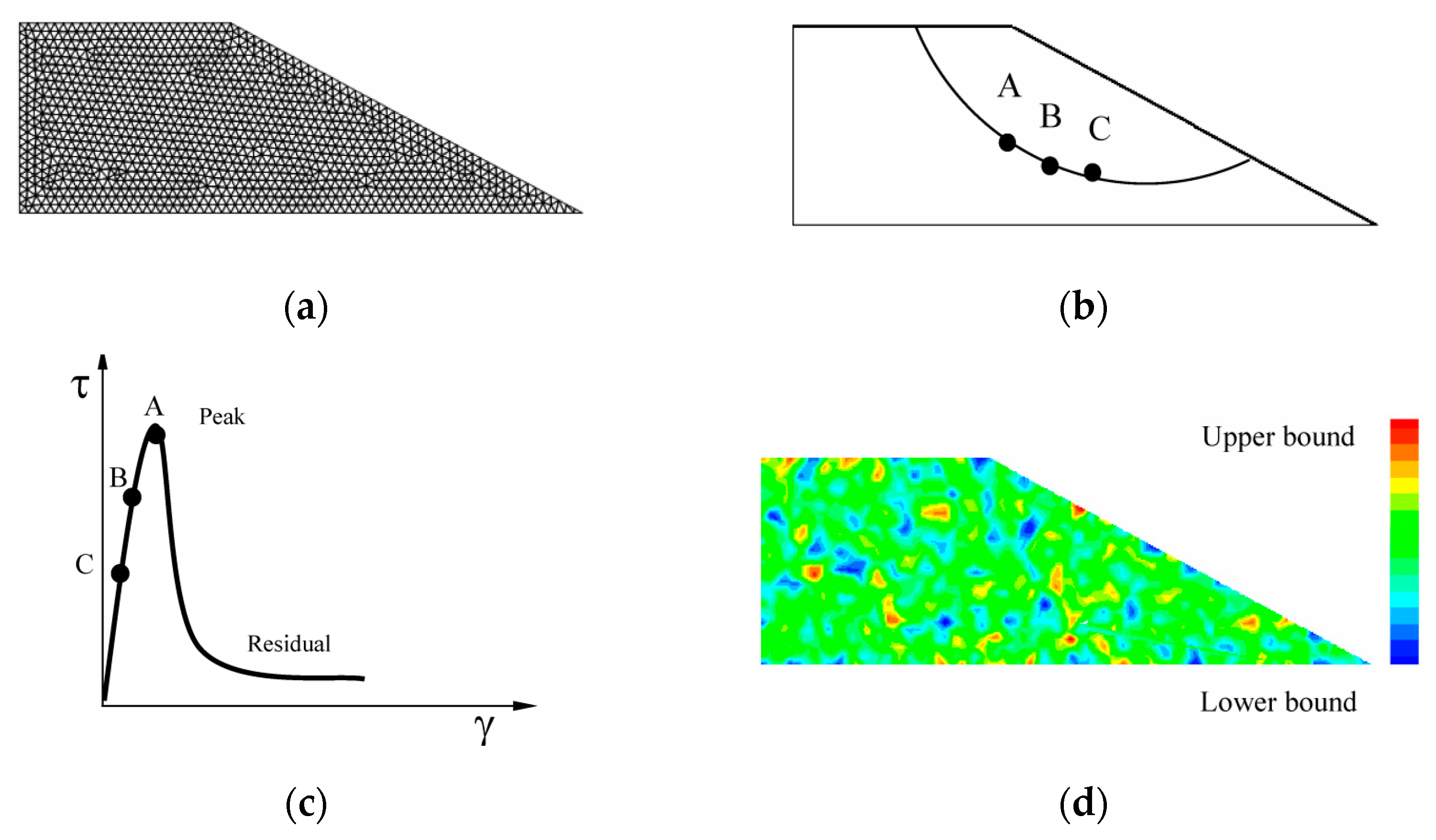
Figure 4.
Progressive fracture phenomena through a series of components: (a) evolution of the domain boundary, (b) implementation of a new scheme within the FEM, and (c) discretization scheme applied. (Note: The red lines indicate fracture paths).
Figure 4.
Progressive fracture phenomena through a series of components: (a) evolution of the domain boundary, (b) implementation of a new scheme within the FEM, and (c) discretization scheme applied. (Note: The red lines indicate fracture paths).

Figure 5.
Computation of the fracture response in heterogenous soil slope conditions.
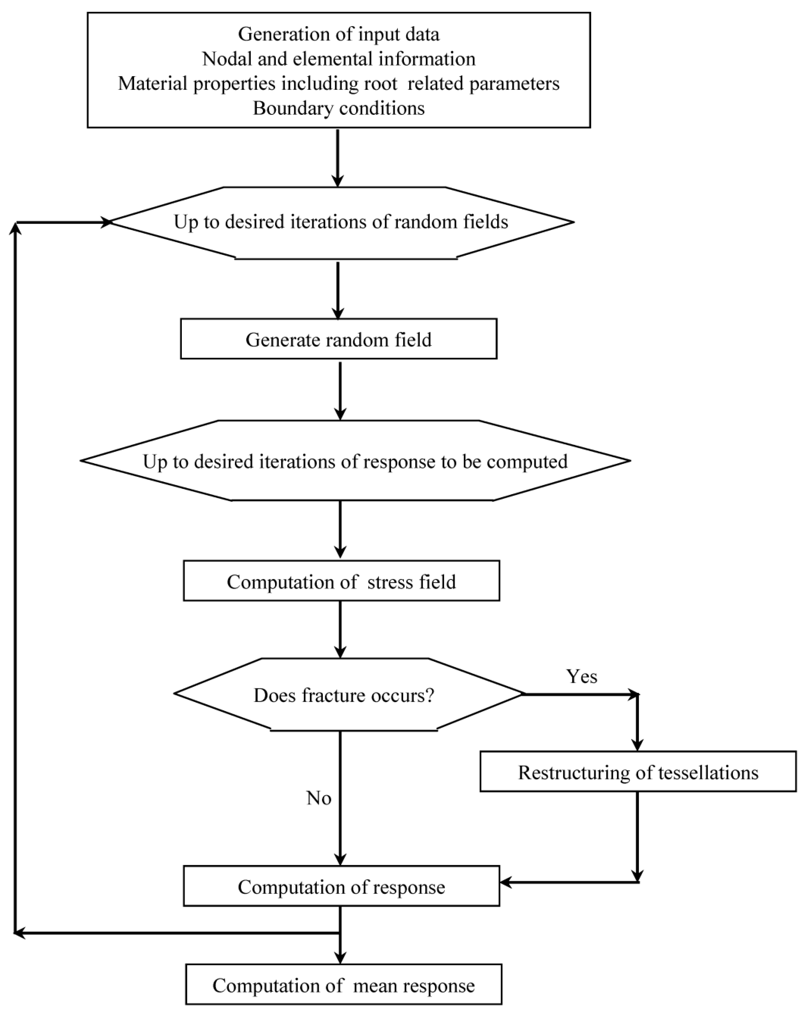
Figure 6.
The soil slope model incorporates a meshing scheme that includes a designated zone for root reinforcement. This meshing scheme allows for the accurate representation and analysis of the impact of root reinforcement on slope stability.
Figure 6.
The soil slope model incorporates a meshing scheme that includes a designated zone for root reinforcement. This meshing scheme allows for the accurate representation and analysis of the impact of root reinforcement on slope stability.
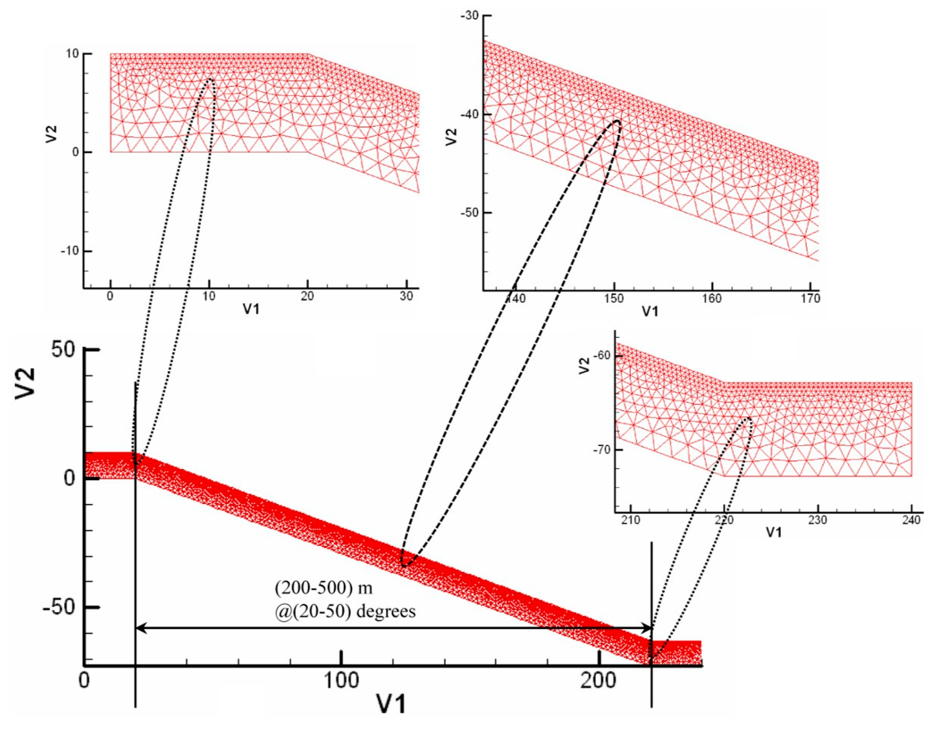
Figure 7.
The progressive failure surface of a slope with a 0.6% RAR and an inclination angle of 30 degrees. The failure process is visualized in four distinct stages: (a) Failure Stage 1: the initial stage of failure; (b) Failure Stage 2: the progression of failure beyond the initial stage; (c) Failure Stage 3: the final stage of failure.

Figure 8.
The progressive failure phenomena observed in a stochastic FEM analysis of a 30-degree slope with a 0.6% RAR. The key stages of failure are highlighted as follows: (a) Typical Failure Stage: this stage showcases the characteristic black region, representing the failure zone within the domain; (b) Failure Portion: this view provides a wider perspective, highlighting the extent of the failure portion within the analyzed domain and clearly illustrating the distinct failed elements and nodes, with the propagation of fractures along the edges of the Delaunay tessellations.
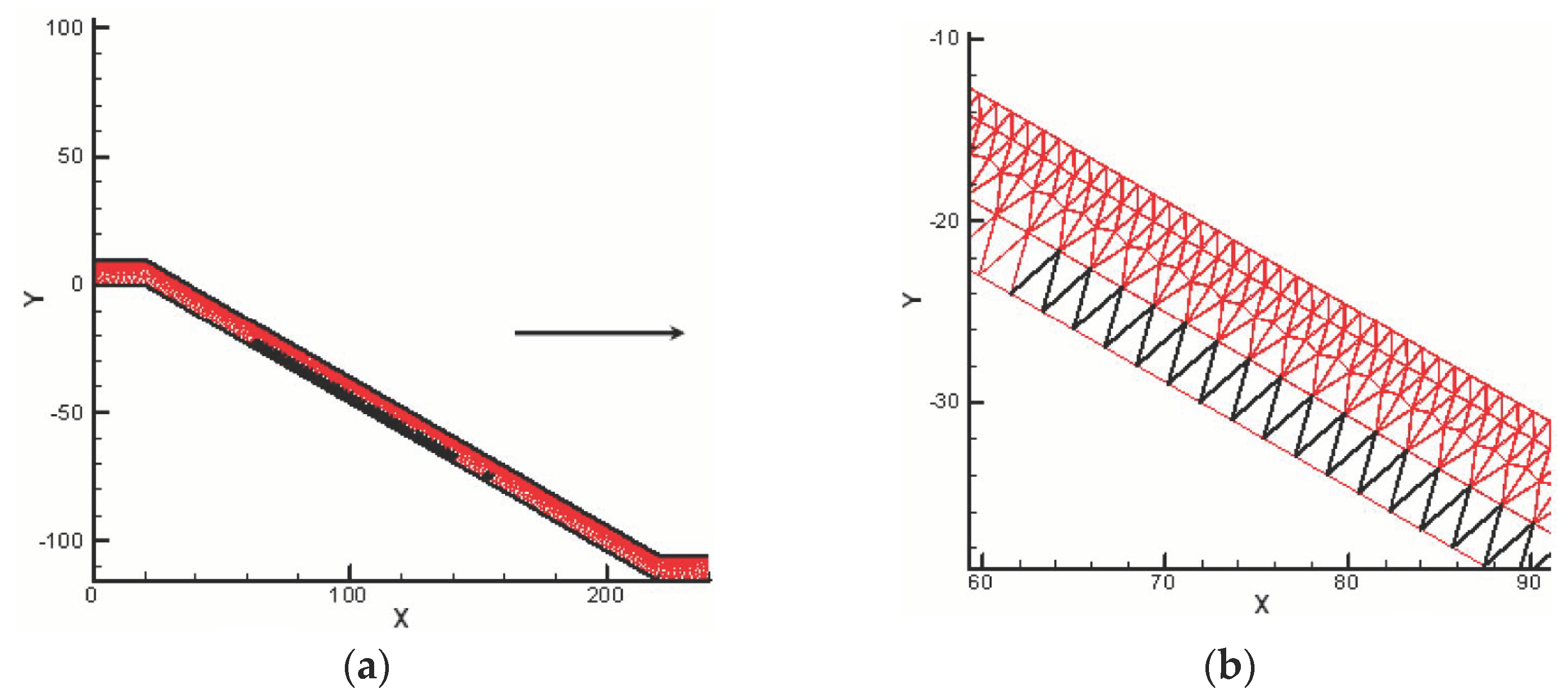
Figure 9.
The typical progressive displacement fields (the first displacement component u1 in meters) along the x-axis (in meters) for a 30-degree slope with a 0.6% RAR using stochastic FEM are presented. The displacement fields are shown for three distinct failure stages, namely: (a) Failure Stage 1; (b) Failure Stage 2; and (c) Final Failure Stage 3.

Figure 10.
Progressive displacement fields (the second displacement component u2 in meters) of a 30-degree slope with 0.6% RAR by stochastic FEM: (a) Failure Stage 1: initial phase of failure; (b) Failure Stage 2: subsequent phase of failure; (c) Failure Stage 3: final stage of failure.
Figure 10.
Progressive displacement fields (the second displacement component u2 in meters) of a 30-degree slope with 0.6% RAR by stochastic FEM: (a) Failure Stage 1: initial phase of failure; (b) Failure Stage 2: subsequent phase of failure; (c) Failure Stage 3: final stage of failure.
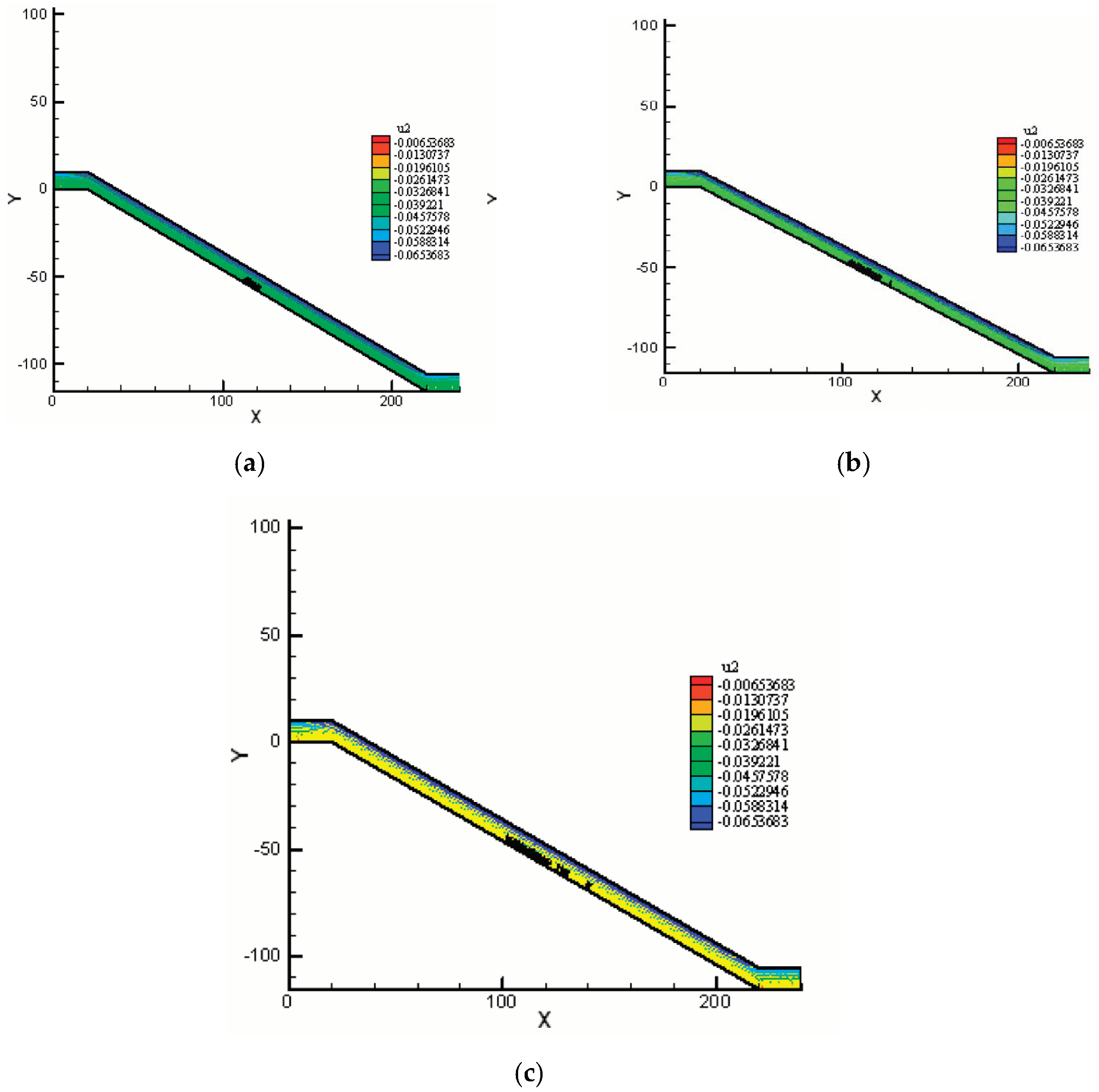
Figure 11.
Progressive stress field (kN/m2) of a 30-degree slope with 0.6% RAR by stochastic FEM: (a) Failure Stage 1: initial phase of failure; (b) Failure Stage 2: progression of failure; (c) Failure Stage 3: final stage of failure.
Figure 11.
Progressive stress field (kN/m2) of a 30-degree slope with 0.6% RAR by stochastic FEM: (a) Failure Stage 1: initial phase of failure; (b) Failure Stage 2: progression of failure; (c) Failure Stage 3: final stage of failure.
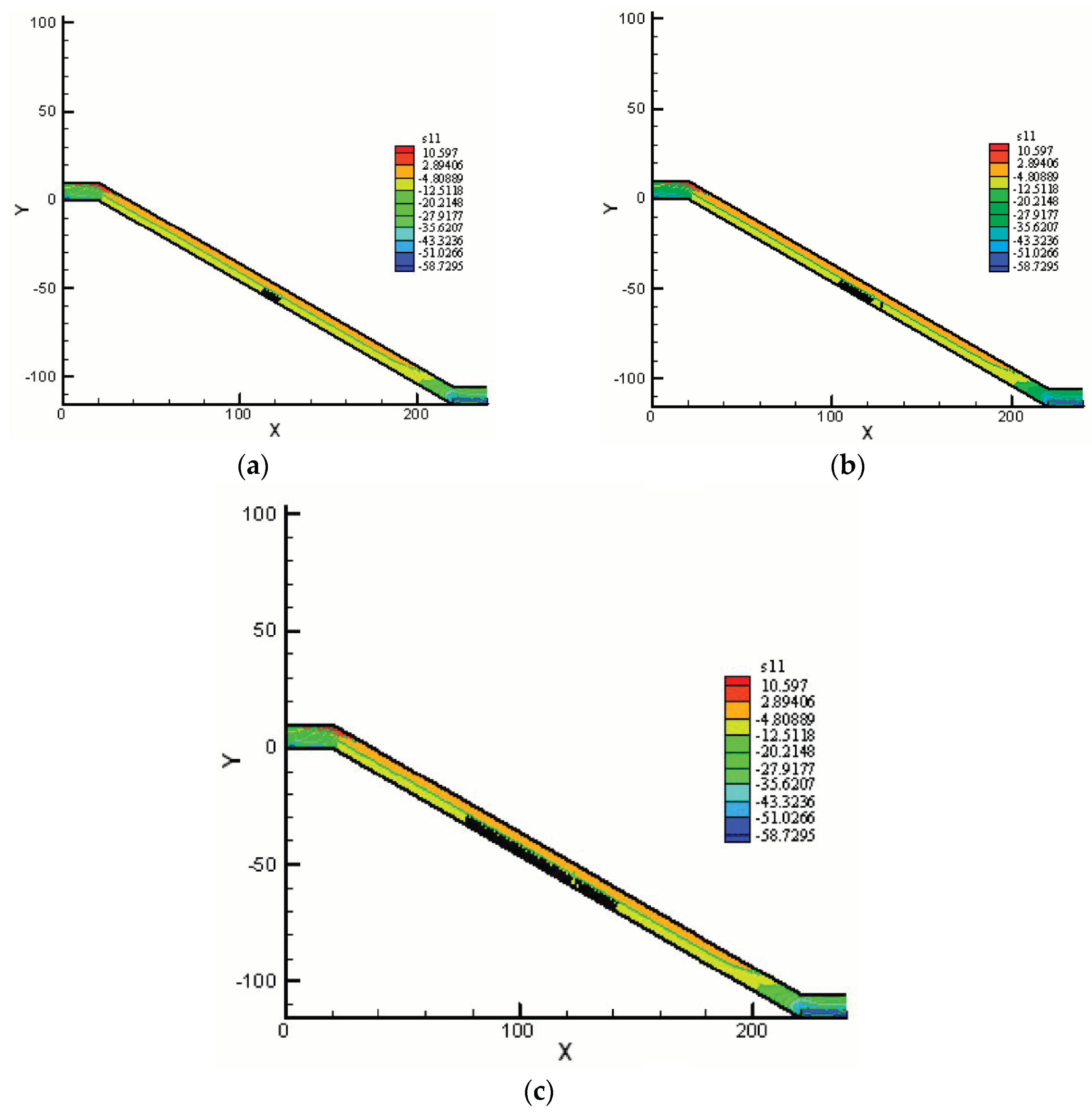
Figure 12.
Progressive stress field (kN/m2) of a 30-degree slope with 0.6% RAR by stochastic FEM: (a) Failure Stage 1: stress distribution at the initial stage of failure; (b) Failure Stage 2: evolving stress distribution as failure progresses; (c) Final Failure Stage 3: ultimate stress distribution within the slope.
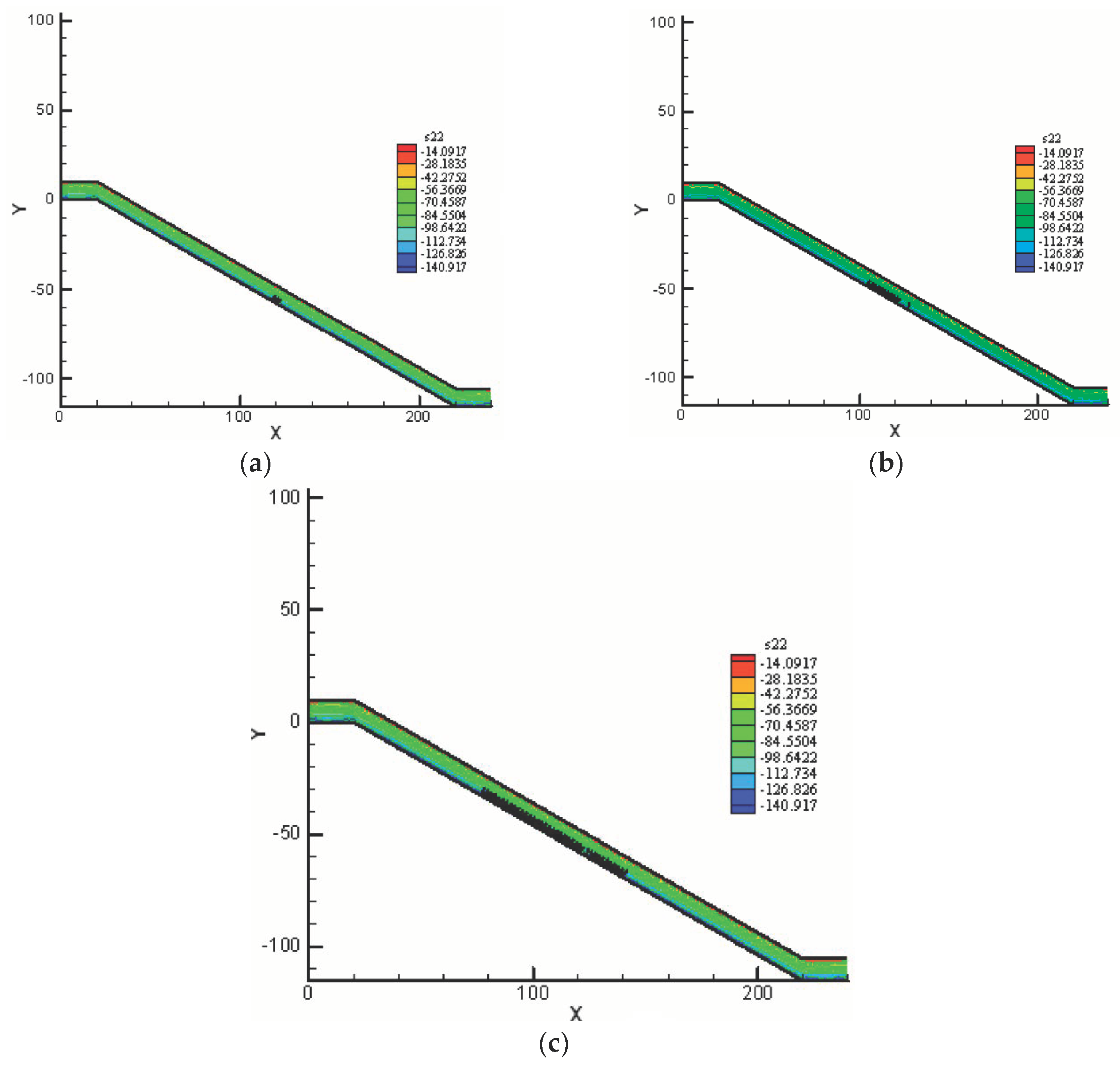
Figure 13.
Progressive stress field (kN/m2) of a 30-degree slope with 0.6% RAR by stochastic FEM: (a) Failure Stage 1: initial stress distribution within the slope; (b) Failure Stage 2: evolving stress distribution as failure progresses; (c) Failure Stage 3: final stress distribution within the slope.
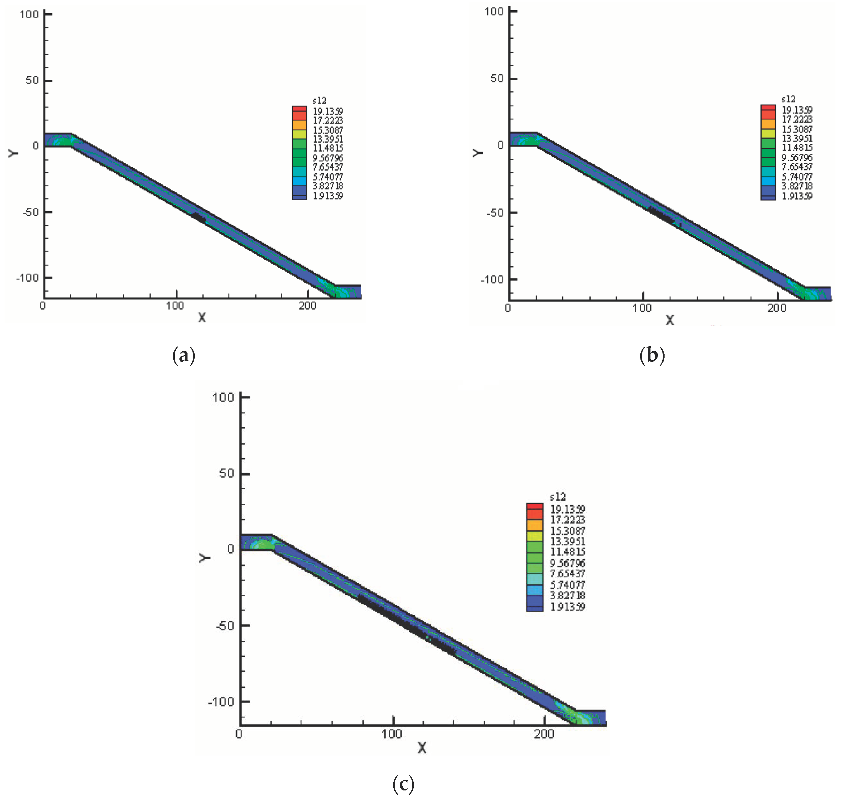
Figure 14.
The typical progressive factor of safety for a 30-degree dry slope composed of USCS soil type CL-ML, with a RAR of 0.6%.
Figure 14.
The typical progressive factor of safety for a 30-degree dry slope composed of USCS soil type CL-ML, with a RAR of 0.6%.
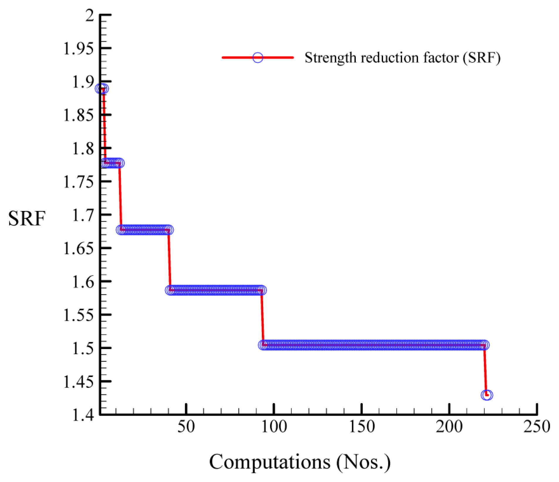
Figure 15.
Stochastic interpretations of the root-reinforcement effect using a 0.6% RAR in a 30-degree dry slope composed of USCS soil type CL-ML: (a) pdf diagram; (b) cdf diagram.
Figure 15.
Stochastic interpretations of the root-reinforcement effect using a 0.6% RAR in a 30-degree dry slope composed of USCS soil type CL-ML: (a) pdf diagram; (b) cdf diagram.
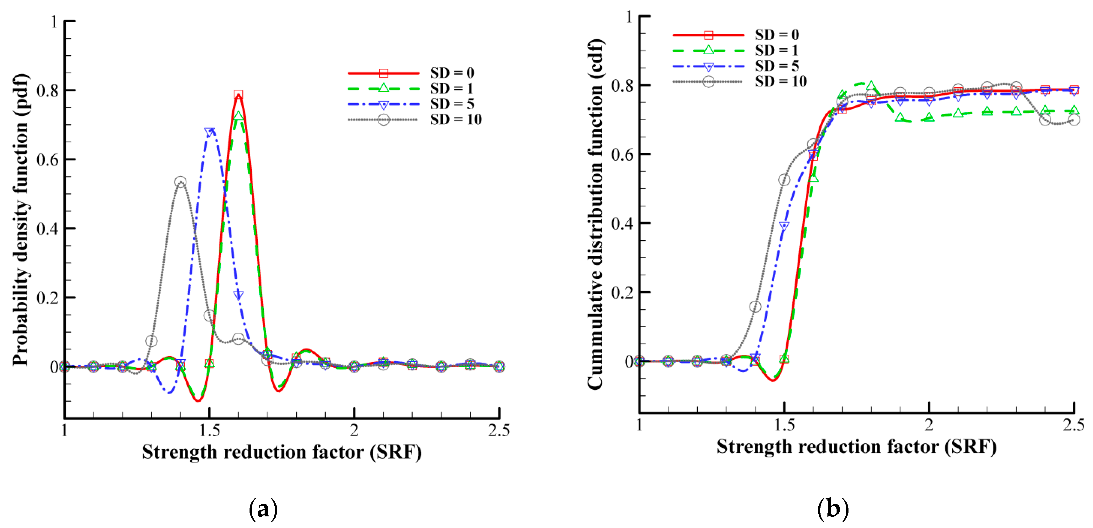
Figure 16.
Stochastic interpretations of the root-reinforcement effect using a 0.7% RAR in a 30-degree dry slope composed of USCS soil type CL-ML: (a) pdf diagram, (b) cdf diagram.
Figure 16.
Stochastic interpretations of the root-reinforcement effect using a 0.7% RAR in a 30-degree dry slope composed of USCS soil type CL-ML: (a) pdf diagram, (b) cdf diagram.

Figure 17.
Stochastic interpretations of the root-reinforcement effect using a 0.8% RAR in a 30-degree dry slope composed of USCS soil type CL-ML: (a) pdf diagram; (b) cdf diagram.
Figure 17.
Stochastic interpretations of the root-reinforcement effect using a 0.8% RAR in a 30-degree dry slope composed of USCS soil type CL-ML: (a) pdf diagram; (b) cdf diagram.

Figure 18.
Stochastic interpretations of root-reinforcement effect with RAR ranging from 0.1% to 0.5% on a 20 degrees slope at a standard deviation of 1: (a) The pdf diagram: (b) The cdf diagram.
Figure 18.
Stochastic interpretations of root-reinforcement effect with RAR ranging from 0.1% to 0.5% on a 20 degrees slope at a standard deviation of 1: (a) The pdf diagram: (b) The cdf diagram.
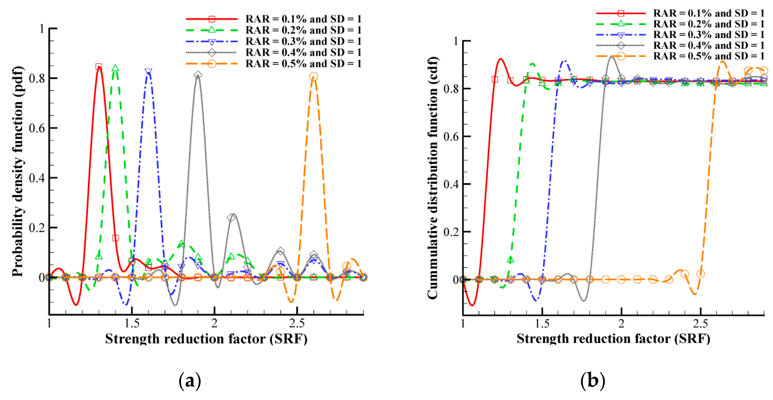
Figure 19.
Stochastic interpretations of root-reinforcement effect with RAR ranging from 0.1% to 0.5% on a 20-degree slope with a standard deviation of 5: (a) The pdf diagram: (b) The cdf diagram.
Figure 19.
Stochastic interpretations of root-reinforcement effect with RAR ranging from 0.1% to 0.5% on a 20-degree slope with a standard deviation of 5: (a) The pdf diagram: (b) The cdf diagram.
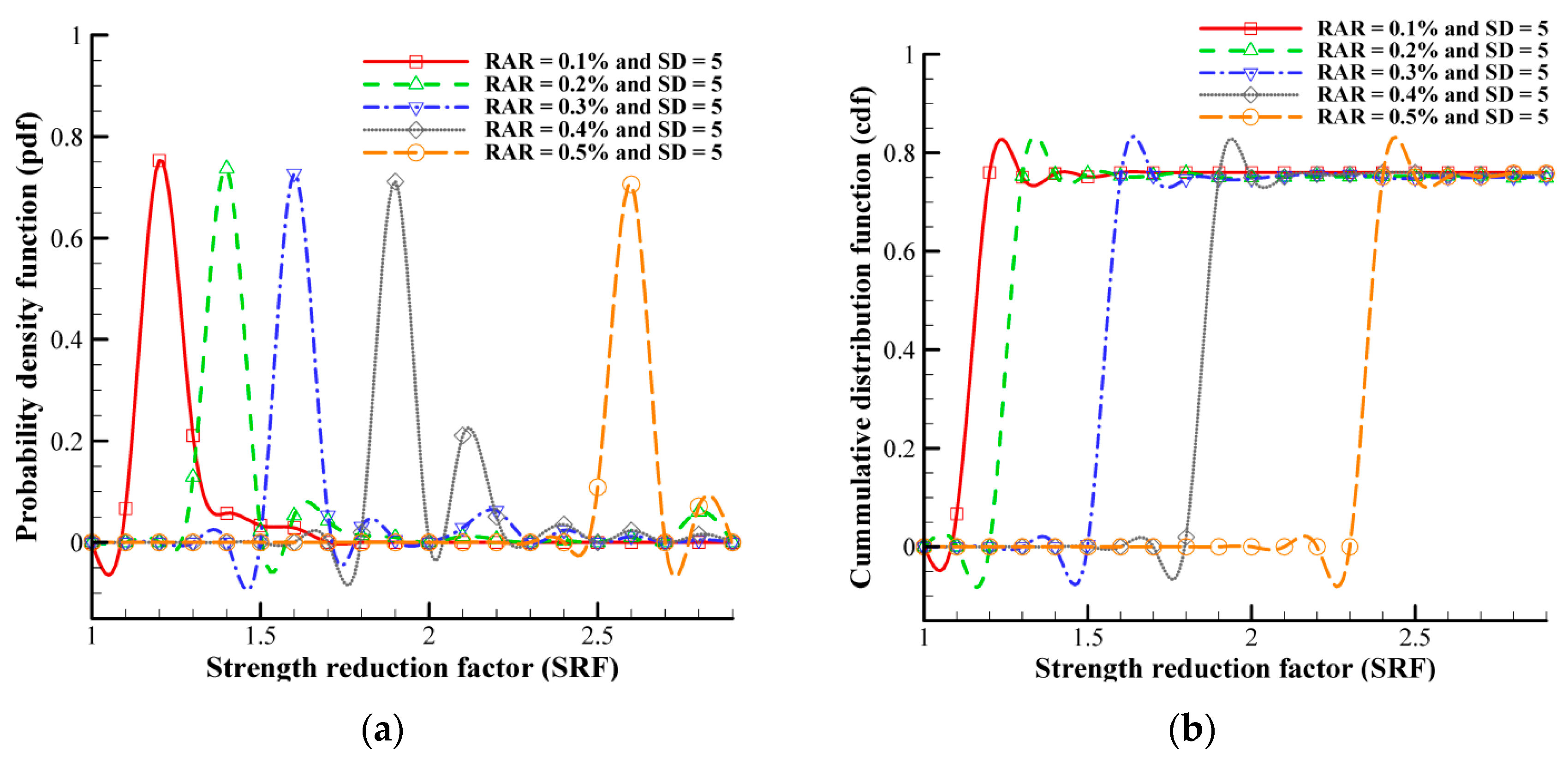
Figure 20.
Stochastic interpretations of root-reinforcement effect with RAR ranging from 0.1% to 0.5% on a 25-degree slope with a standard deviation of 1: (a) The pdf diagram: (b) The cdf diagram.
Figure 20.
Stochastic interpretations of root-reinforcement effect with RAR ranging from 0.1% to 0.5% on a 25-degree slope with a standard deviation of 1: (a) The pdf diagram: (b) The cdf diagram.
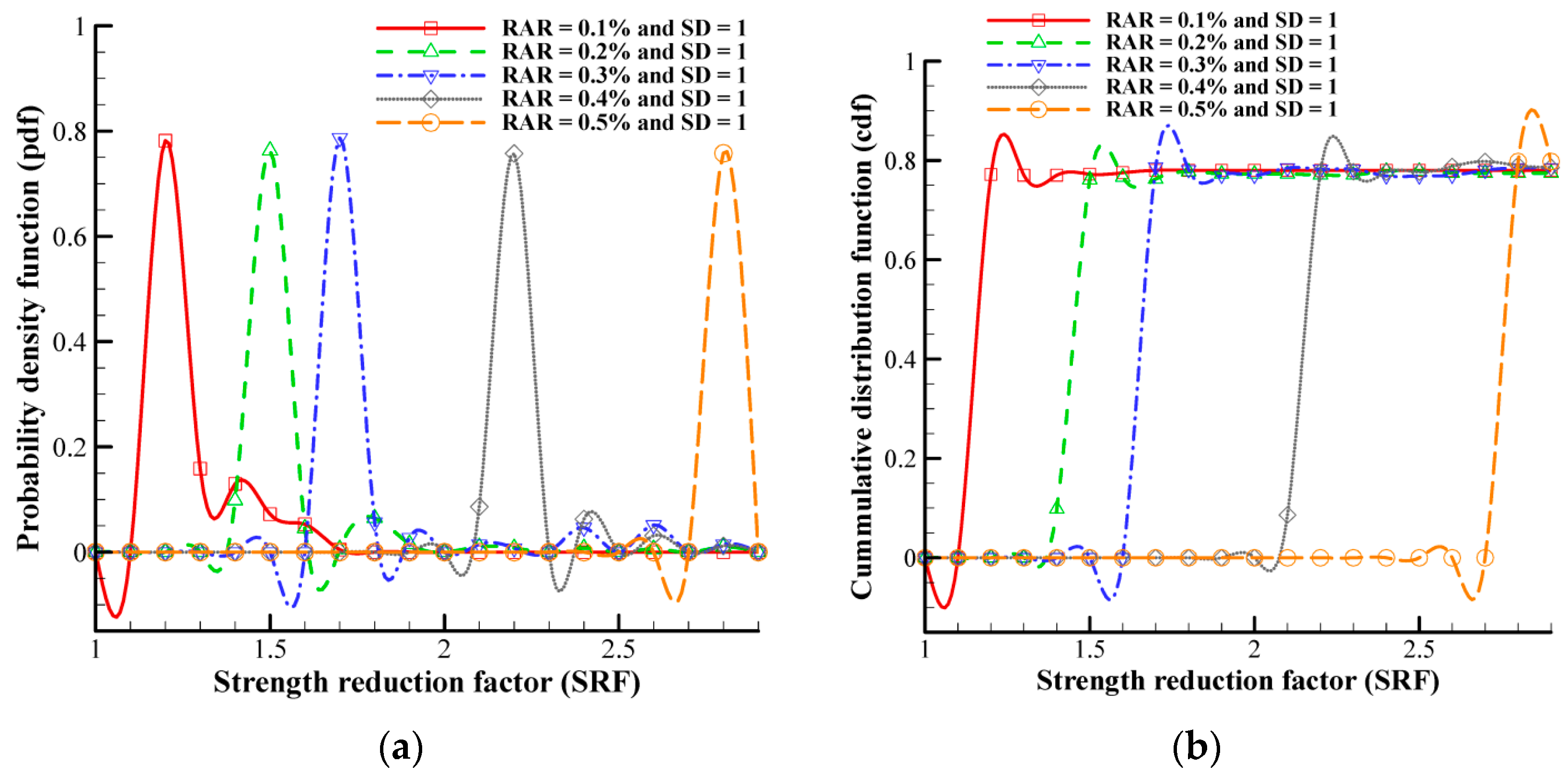
Figure 21.
Stochastic interpretations of root-reinforcement effect with RAR ranging from 0.1% to 0.5% on a 25-degree slope with a standard deviation of 5: (a) The pdf diagram: (b) The cdf diagram.
Figure 21.
Stochastic interpretations of root-reinforcement effect with RAR ranging from 0.1% to 0.5% on a 25-degree slope with a standard deviation of 5: (a) The pdf diagram: (b) The cdf diagram.
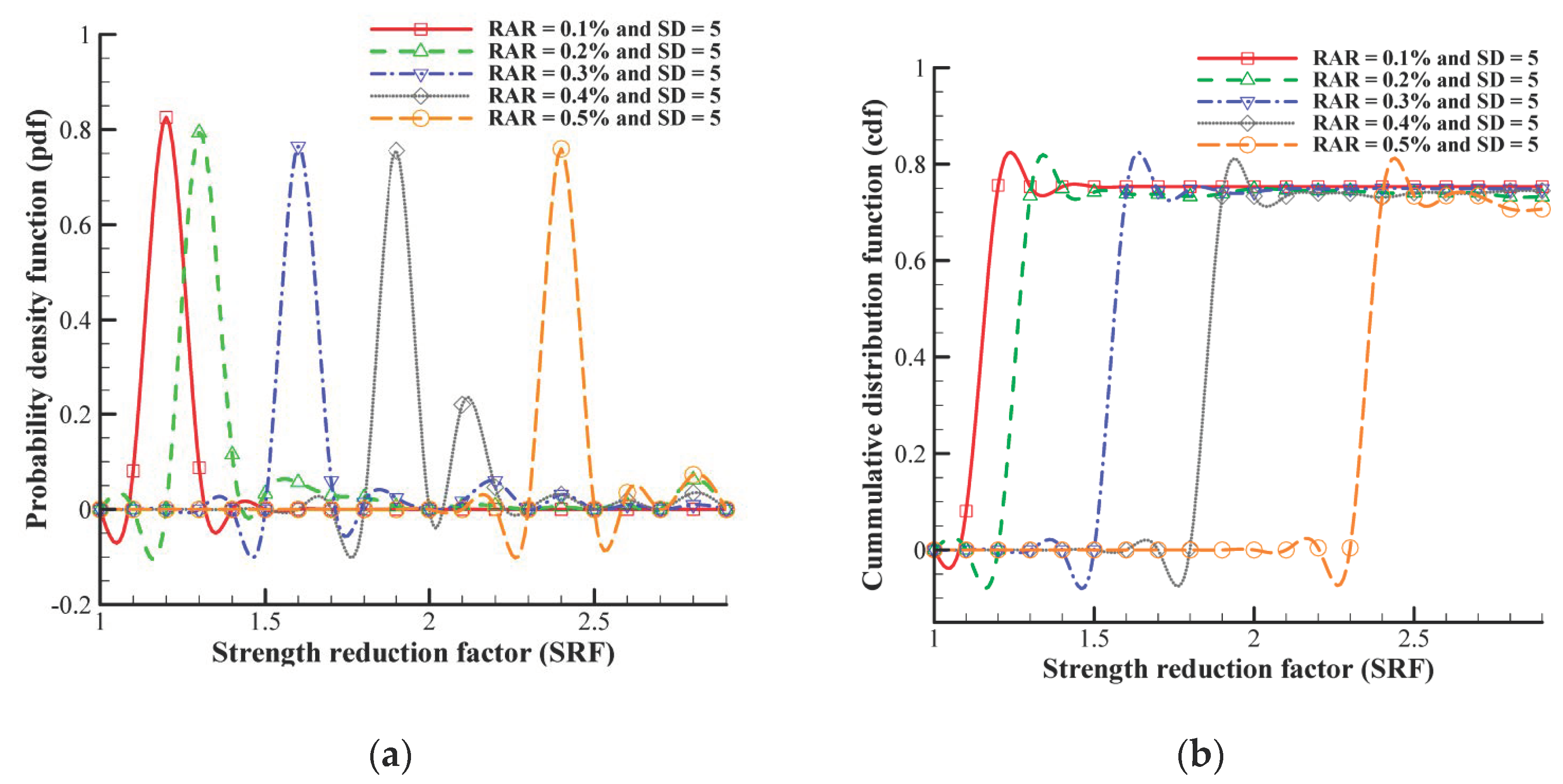
Figure 22.
Stochastic interpretations of a 30-degree slope with a material model of USCS clayey silt (CL) at standard deviation values ranging from 1 to 20: (a) pdf diagram: (b) cdf diagram.
Figure 22.
Stochastic interpretations of a 30-degree slope with a material model of USCS clayey silt (CL) at standard deviation values ranging from 1 to 20: (a) pdf diagram: (b) cdf diagram.
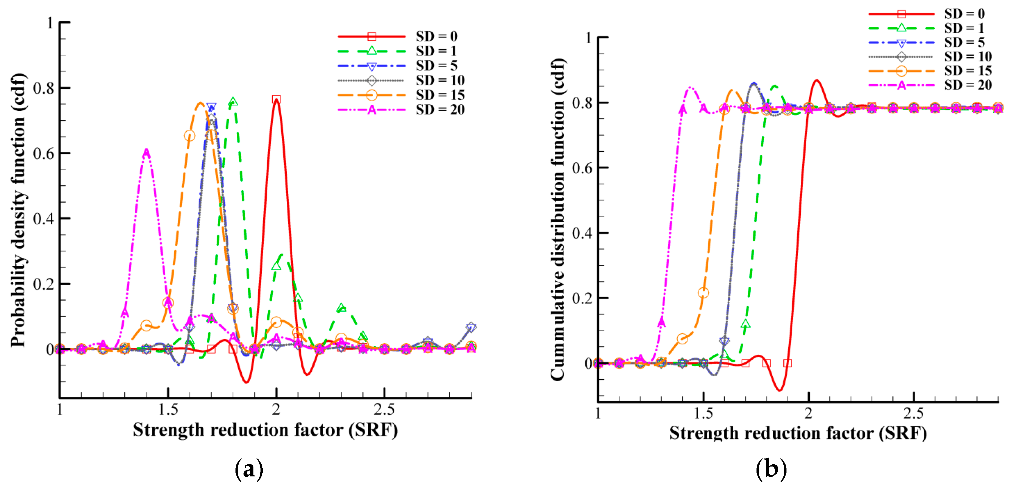
Figure 23.
Stochastic interpretations of a 30-degree slope with a material model of USCS clay soil (CH) at standard deviations ranging from 1 to 10: (a) pdf diagram: (b) cdf diagram.
Figure 23.
Stochastic interpretations of a 30-degree slope with a material model of USCS clay soil (CH) at standard deviations ranging from 1 to 10: (a) pdf diagram: (b) cdf diagram.
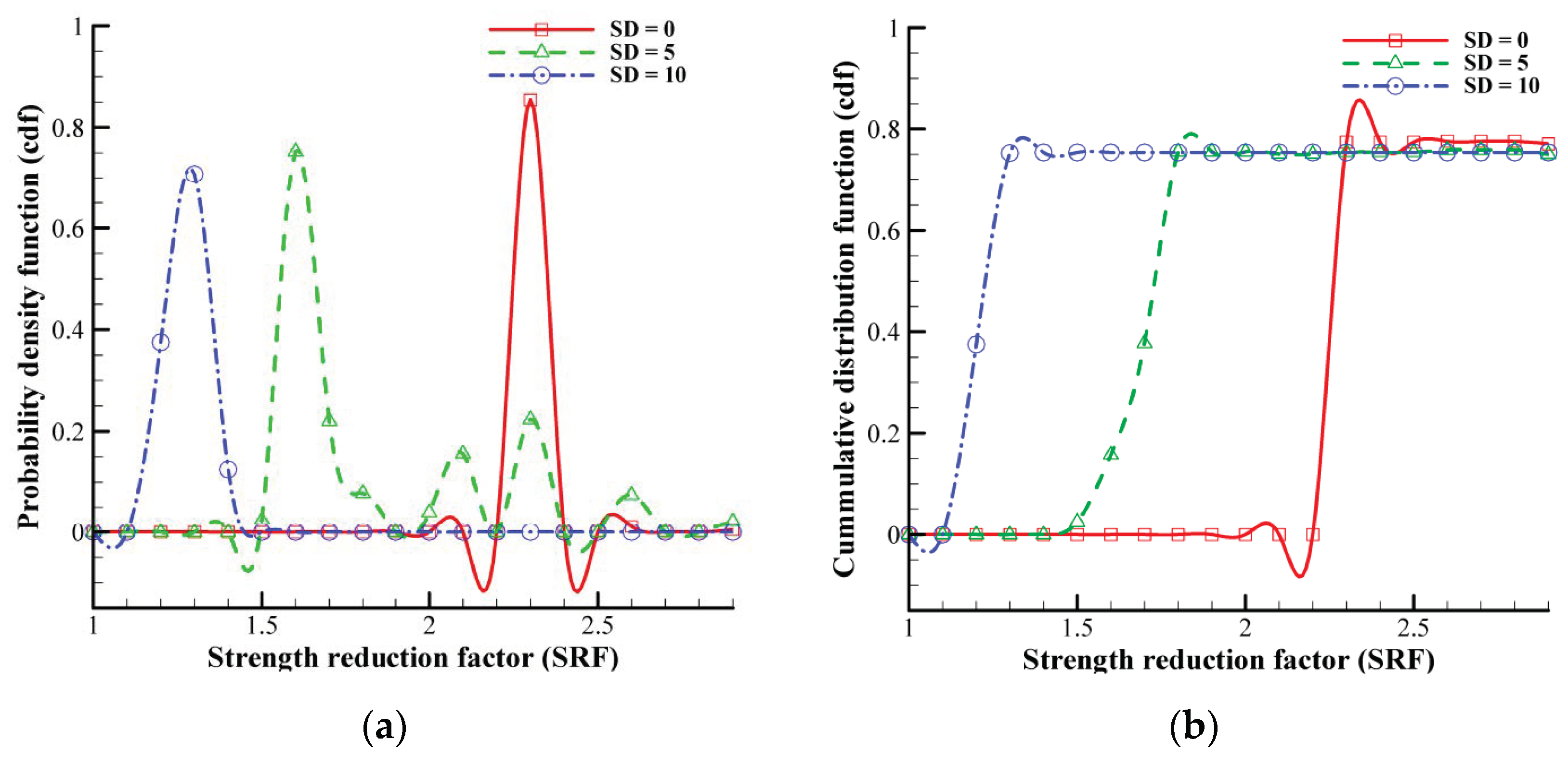
Figure 24.
Stochastic interpretations of 25-degree and 30-degree slopes with a material model of USCS clay soil (CH) at standard deviations ranging from 1 to 10: (a) pdf diagram: (b) cdf diagram.
Figure 24.
Stochastic interpretations of 25-degree and 30-degree slopes with a material model of USCS clay soil (CH) at standard deviations ranging from 1 to 10: (a) pdf diagram: (b) cdf diagram.


Disclaimer/Publisher’s Note: The statements, opinions and data contained in all publications are solely those of the individual author(s) and contributor(s) and not of MDPI and/or the editor(s). MDPI and/or the editor(s) disclaim responsibility for any injury to people or property resulting from any ideas, methods, instructions or products referred to in the content. |
© 2023 by the authors. Licensee MDPI, Basel, Switzerland. This article is an open access article distributed under the terms and conditions of the Creative Commons Attribution (CC BY) license (https://creativecommons.org/licenses/by/4.0/).
Share and Cite
MDPI and ACS Style
Tiwari, R.C.; Bhandary, N.P. Stochastic Finite Element Analysis of Root-Reinforcement Effects in Long and Steep Slopes. Geotechnics 2023, 3, 829-853. https://doi.org/10.3390/geotechnics3030045
AMA Style
Tiwari RC, Bhandary NP. Stochastic Finite Element Analysis of Root-Reinforcement Effects in Long and Steep Slopes. Geotechnics. 2023; 3(3):829-853. https://doi.org/10.3390/geotechnics3030045
Chicago/Turabian StyleTiwari, Ram Chandra, and Netra Prakash Bhandary. 2023. "Stochastic Finite Element Analysis of Root-Reinforcement Effects in Long and Steep Slopes" Geotechnics 3, no. 3: 829-853. https://doi.org/10.3390/geotechnics3030045