Exchangeable Quantities and Power Laws: Τhe Case of Pores in Solids

Abstract

In this work we suggest that the common cause for the development of various power laws is the existence of a suitable exchangeable quantity between the agents of a set. Examples of such exchangeable quantities, leading to eponymous power laws, include money (Pareto’s Law), scientific knowledge (Lotka’s Law), people (Auerbach’s Law), and written or verbal information (Zipf’s Law), as well as less common cases like bullets during deadly conflicts, recognition in social networks, heat between the atmosphere and sea-ice floes, and, finally, mass of water vapors between pores in solids. This last case is examined closely in the present article based on extensive experimental data. It is shown that the transferred mass between pores, which eventually grow towards a power law distribution, may be expressed using different parameters, either transferred surface area, or transferred volume, or transferred pore length or transferred pore anisotropy. These distinctions lead to different power laws of variable strength as reflected by the corresponding exponent. The exponents depend quantitatively on the spread of frequency distribution of the examined parameter and tend to zero as the spread of distribution tends to a single order of magnitude. A comparison between the energy and the entropy of different kinds of pore distributions reveals that these two statistical parameters are linearly related, implying that the system poise at a critical state and the exchangeable quantities are the most convenient operations helping to keep this balance.

1. Introduction

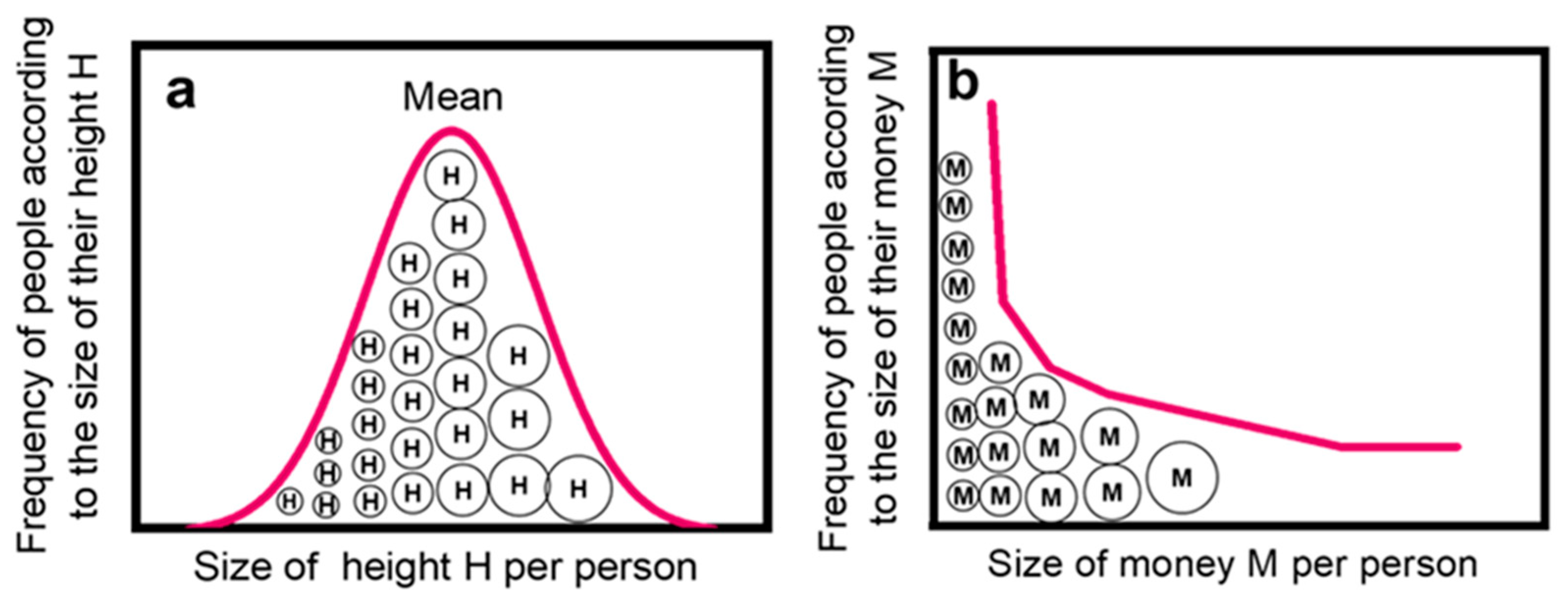
Power laws are observed in many datasets of objects, phenomena, or i events whose number, N_i, appear inversely to their size, S_i, and therefore do not accumulate randomly around a central value as highlighted by Newman [1]. In this last case, the random build-up of S_i values symmetrically around a mean value S_mean usually yields an approximately normal distribution, as shown schematically in Figure 1a. This outcome suggests that the sizes of the i elements develop separately and do not depend on, or interact with, their neighbors for resources of mass, energy, space, information, money, social recognition, etc. Relevant examples are people’s heights, student’s grades, and speeds of cars: people do not exchange heights, students should not share information during exams, and cars do not swap speeds. So, if we plot the number of people vs. their heights, or the number of students vs. the corresponding grades, or the numbers of cars vs. their speeds, we obtain a more or less Gaussian distributions N_i = [1/σ·(2π)^0.5]·exp[−(S_i − S_mean)/2σ²], where symbols have their usual meaning; people’s heights are commonly accumulated around a central value 170–180 ± 20 cm, student’s grades in 0–10 scale usually lay within 5–6 ± 3, and the speed of cars usually ranges in the vicinity 80–100 ± 50 km/h.

Another common case is that the i elements of the dataset may interact with each other and exchange some quantity X in a gradual procedure. Such exchangeable quantities, which as mentioned may be people, money, energy, food, bullets, bytes, or a handful of other cases, result to power or quasi-power law distributions of the affected set. Such laws exhibit the general form given by relationship (1) and shown graphically in Figure 1b.

N_i ≈ a/S_i·^q

(1)

where q is a small number, usually 1 < q < 3. Typical cases, initially established by the beginning of 20th century, are the distribution of financial wealth according to Pareto’s Law [2] and the list size of scientific publications by various authors in accordance to Lotka’s Law [3]. The first case is the result of many economic transactions, while the second is the outcome of exchanging scientific information between researchers. Such power law distributions are commonly expressed in logarithmic form according to relation (2).

logN_i ≈ loga − q·logS_i

(2)

Figure 1. Diagram depicting the transformation of a normal distribution (a) of i elements into a power law (b) by introducing an exchangeable quantity. Both dispersals refer to the same dataset of agents (i—people) designated as circles ◯ but describe frequency–size distributions N_i = f(S_i) of different properties. Let the normal distribution in (a) reflect the height H of people Ⓗ, which spreads randomly on either side of a mean value S_mean. This property cannot be exchanged between the members of the group. If an exchangeable quantity, like money Ⓜ, is introduced into the group, the distribution of its members in this novel environment will eventually turn into a power law as seen in (b). The above figures were inspired by the first two figures in the article of Newman [1], as well as by a similar figure in ref. [4] by Barabási.

Figure 1. Diagram depicting the transformation of a normal distribution (a) of i elements into a power law (b) by introducing an exchangeable quantity. Both dispersals refer to the same dataset of agents (i—people) designated as circles ◯ but describe frequency–size distributions N_i = f(S_i) of different properties. Let the normal distribution in (a) reflect the height H of people Ⓗ, which spreads randomly on either side of a mean value S_mean. This property cannot be exchanged between the members of the group. If an exchangeable quantity, like money Ⓜ, is introduced into the group, the distribution of its members in this novel environment will eventually turn into a power law as seen in (b). The above figures were inspired by the first two figures in the article of Newman [1], as well as by a similar figure in ref. [4] by Barabási.

The above proposition implies that if a group N of i agents, for example, people, is characterized by a property X, like height H, which is not exchangeable between them, then the frequency N_i of values of that specific property (height per person) is randomly scattered around a central value S_mean yielding roughly a normal distribution. However, if the same group of people is furnished with a novel exchangeable quantity, like money M, and start exchanging it, not quite randomly but to gain some kind of advantage, then the size S_i of economic health per person, after extensive financial transactions between the group’s members, is eventually developed into a power or quasi-power law. This transformation is depicted in Figure 1.

On the same token, if a group of students is examined as to their sole knowledge (exam markings) without any interaction, the result shall be a more or less a normal distribution. However, if exchange and accumulation of knowledge is allowed via interaction with peers, books, or the Internet, then the gained and accumulated knowledge (scientific publications) of students (or at least some of them) will eventually develop towards a power law or a quasi-power law. In the case of cars, if their fleet is evaluated not according to their speeds, but according to their prices, we shall obtain some kind of power law distribution: there are few Porches and Lamborghinis and many humble cars in the streets, but clearly this case leads back to the exchangeable property of money.

It is emphasized that it is not necessary for the distribution in Figure 1a to be of normal type; it may actually exhibit any irregular arrangement, even a flat one. Nevertheless, the normal distribution paradigm is usually put forward since it reflects many “neat” scientifically quantified statistics. On the contrary, data spread randomly in an irregular fashion and not following a standard mathematical description (i.e., Gauss, Poisson, etc.) are often disregarded as nuisances although they may lead to power laws like that in Figure 1b. For a relevant discussion see [5].

2. Exchangeable Properties

The concept of “Exchangeable Quantities” leading to power laws is a general expression engulfing many different cases. It is understood that some alternative definitions, like “Transferable Quantities” or “Commutable Properties” might express equally well some real-world instances, but for reasons of brevity and simplicity we shall stick to the first definition. To the best of our knowledge, the only suggestion relevant to the present proposal, namely that exchangeable quantities lead to power laws, has been put forward by Chatterjee et al. in [6]. These authors suggested that wealth distribution in various societies resembles the Maxwell–Boltzmann distribution of energy in an ideal gas. They consider economy as an exchange game of different commodities and treat the corresponding money trading as a scattering event between gas molecules which exchange energy, that is, money (this concept is sometimes called econophysics). Under specific conditions, this model leads to a power law.

Exchangeable advantageous quantities, apart from money (leading to Pareto’s Law) and knowledge (leading to Lotka’s Law) mentioned above, may be people themselves in the case of human settlements according to the original Auerbach suggestion [7]; written or verbal information in the case of language leading to the celebrated Zipf Law [8,9]; geological stress and friction (e.g., energy) between tectonic plates in the case of earthquakes leading to the Richter scale [10]; resources in breeding populations leading to genetic drift in biological taxa, known as the Yule process [11,12]; bytes of information in IT technologies like Internet networks, web pages, links to them, and hits in web sites, termed collectively as Complex Networks [13]; flares in forest fires [1,12]; bullets and other deadly projectiles during wars [14,15]; common beliefs in religious denominations, bodies, and sects [1,14]; social recognition (likes) of individuals like actors, personas, and politicians in social networks via modern electronic applications like FB, Twitter, etc. [16]; musical notes, colors, and shapes in music and painting [16,17]; food along the trophic chain of pelagic species (phytoplankton, zooplankton, and fishes) [18,19]; athletic equipment, tools, or objects (balls, disks, javelins, etc.) used in competitive sports in respect to the resulting power law medal ranking [20], as well as to the achieved human endurance [21]; and, last but not least, energy and heat between the atmosphere and ocean, which drives the power law distribution of sea-ice floes in Arctic seas [22,23].

The latest addition to this litany of power laws is the Zipfian relationship N_i ≈ 1/V_i observed between the differential numbers N_i and the volumes V_i (≡sizes S_i) of pores in solids, which is the main subject of this work. In this case, the exchangeable quantity is the fluid content (usually water vapor but sometimes also CO₂) of evolving pores that coalesce step by step towards larger ones as encountered, for example, in volcanic magma, drying soils, or lab made sol-gels [24,25,26,27,28]. The gain in this case is the relaxation of surface tension, which decreases inversely to the pore radius according to the Young–Laplace equation.

Cases of above power laws, where the exchangeable quantity is energy or mass, are reminiscent of the so-called constructal law of design and evolution in nature, suggested in a number of publications by Bejan and Lorente [29,30,31]. According to these authors, many diverse animate, inanimate, or engineered designs, described by Zipf’s distributions (e.g., power laws), are a manifestation of the constructal law in the generation of those designs that facilitate, among other things, the flow of water in nature, including rivers, trees, and the human body, as well as the distribution of city sizes (S_i) and numbers (N_i) in various geographical areas like continents and states.

The proposition of exchangeable quantities can be only ensured via some kind of interaction between at least two participating agents. Therefore, it is closely related to the creation of efficient interactive networks which, as discussed thoroughly by Barabasi in [4], result in scale-free structures. For example, in [4], the author summarizes the well-known paradigm of www connecting various computer hubs around the globe, as an efficient network for exchanging various information quantities. Without efficient networks, the exchangeable quantities are null and void. Nevertheless, it is the various human pursuits (for example efficient exchange of information via www) or/and different physical necessities (for example efficient flow of fluids in the labyrinth of pores) that drive the creation of such efficient networks.

Towards this end, a humorous and self-ironic, but nevertheless penetrating, comment by Fabrikant et al. [32] makes sense: “Power laws…have been termed ‘the signature of human activity’…They are certainly the product of one particular kind of human activity: looking for power laws…” (cited by Mitzenmacher in [33]). Paraphrasing the above, it could be said that power laws are the product of human pursuits, but also of various natural phenomena, that are optimized towards such patterns via exchangeable human activities or transferable natural quantities, or properties, via suitable paths.

There are not many distinct groups of possible quantities suitable for exchangeable operations between living, azoic, or engineered systems. About a dozen such properties have been mentioned above, but their total number cannot be much larger. To this extent, if we categorize the very many cases of power laws encountered in the relevant literature, according to the exchangeable quantity that led to their development, we shall obtain fewer than two dozen archetypal power laws, recognizable through their repeated occurrence and collected into groups that share the same prominent features. Typical examples may be considered the economic sizes of states or the financial health of individuals (exchangeable quantity, money); the population of cities and towns in various areas or states (exchangeable quantity, people); the word’s ranking in texts of human languages (exchangeable quantity, common information); and aspects related to scientific knowledge, like publications, citations, impact factors, and rankings of journals or institutions (exchangeable quantity, specific technical knowledge and data). In ref. [34] an indicative list of about fifteen such archetypal power laws has been put forward.

The purpose of this work is to look into some power laws’ inter-relating properties of porous materials by taking into account the aforementioned ideas of exchangeable quantities controlling their development. The typical pore properties to be considered are pore diameters D_i (cm), specific pore volumes V_i (cm³·g⁻¹), specific surface areas S_i (m²·g⁻¹), specific pore lengths L_i (cm·g⁻¹), and specific pore numbers N_i (g⁻¹). That last property for isotropic pores (e.g., spherical) corresponds to specific pore anisotropies B_i = L_i/D_i (g⁻¹), in other words N_i ≡ B_i. The term “specific” reflects the fact that the relevant property is estimated per unit mass of porous substance and the subscript (i) means that the property is differential with respect each segment of pore sizes.

The structure of the following text is as follows. In Section 3, we present the porous materials and their experimental properties to be employed in the ensuing sections. In Section 4, we show that a practically perfect Zipf’s law N ≈ 1/V between pore density N_i (pores/g) and pore volume V_i (nm³/pore) holds over 17 orders of magnitude for 297 experimental points from twelve (12) porous materials belonging to five (5) different categories of porous samples. In Section 5, we examine the meaning of cumulative and differential power laws and show that these expressions lead to the realization that the exchangeable quantity, that is the mass of pore content in our case, when expressed in different ways, (i.e., pore surface area, pore length, or pore number), leads to different power laws. Finally, in Section 6, we scrutinize the relation between the hidden variables with the exchanged quantities, as well as the energies E_i and entropies S_i of the examined pore property distributions and the relation between them.

3. Experimental Data

The experimental data to be used in the present study are taken from some recent investigations referring to power laws of pores in solids [24,25,26,27,28,34]. They represent twelve (12) kinds of porous materials that belong to five (5) different classes, and are shown in Table 1. Briefly they are the following.

(i)

Three (3) microporous spinels CoAl₂O₄ code named S-500, S-700, and S-900. They were prepared in the lab as reported previously [24,25,26,27,28] and possess pore diameters in the nm sale. The differential surface areas S_i (m²/g) and pore volumes V_i (cm³/g) were determined via standard nitrogen porosimetry using the BET methodology and the BJH algorithm at various partial pressures 0 < (P/Po) = P_i < 1, as described in various standard textbooks [35,36]. From those original parameters, we estimated the differential values of pore diameters D_i = [V_i/S_i] (cm) of pore lengths L_i = [S_i²]/[V_i] (cm/g) and the pore numbers N_i (pores/g), which for isotropic (e.g., spherical) pores tally with the pore anisotropies B_i = [S_i³]/[V_i²] (g⁻¹). The values of D_i and B_i ≡ N_i to be employed in the next graphs and discussion are cited in Table S1. The corresponding values of S_i, V_i, and L_i are too many and are not shown for the sake of space.

(ii)

One (1) mesoporous soil sample with pore diameters in the mm scale. The data were read from Figure 5 in a paper by Wang et al. [37] and estimated as explained in ref [34]. The determination of differential pore diameters D_i and pore numbers N_i encountered in this porous soil took place using Mercury Intrusion Porosimetry (MIP) and the Pressure Plate Test (PPT) [37]. It is mentioned that the porosity of the soil was developed by very slowly decompressing a water-saturated sample at different pressures (P_i = 10, 30, 50, 100, 300, 500, and 1200 kPa), and every pressure step lasted for 12 h in order to achieve equilibrium. The pore sizes D_i were determined via the Washburn equation D_i = (4·σ_s·cosα)/P_i, where σ_s is the surface tension. The values of D_i and N_i are cited in Table S2 and discussed next.

(iii)

Two (2) macroporous volcanic rock mimics, made in the lab with pore openings in the mm–cm scale. The data with code names ET 8 and ET 9 were read out from Figure 4 in a publication by Simakin et al. [38]. These authors employed a gas bomb to study the degassing of water-saturated granite melts at slow rates using a pressure drop from 100 to 40 MPa over 168 h. The purpose was to determine the water exsolution and the vesicle formation. Bubble sizes D_i and numbers N_i were measured in the formed granite glasses using SEM images. The corresponding results D_i and N_i are cited in Table S2 and will be used in the next discussion.

(iv)

Two (2) macroporous magmatic rocks, a Scoria sample from Isola Volcano and a Pumice sample from Etna Volcano, both in Italy. Their pore diameters were in the mm–cm scale. The relevant data D_i and N_i, for Scoria and Pumice samples, which are cited in Table S2 and discussed next, were read from relevant publications by Gaonac’h et al. [39,40,41].

(v)

Four (4) macroporous volcanic magmas from Tarawera Volcano, New Zealand. The data were read from the publication by Sable et al. [42]. The code names of the samples are T28-G4-24, T43-07-67, T47-12-56, and T47-23-35, and their pore diameters are in the mm–cm scale. The relevant data D_i and N_i are cited in Table S2.

It is mentioned that volcanic eruptions, such as those mentioned above for the Etna, Isola, and Tarawera events, are quite violent episodes and the formed magmatic rocks are formed under fast decompression of lava at high temperatures. These conditions affect the cascade of events controlling the pore formation, as will be shown next.

Table 1. The twelve (12) porous materials employed in the present study.

Sample Code Name	Short Description	Ref.
S-500	Lab-made spinel CoAl2O4 heated at 500 °C	[24,25,26,27,28]
S-700	Lab-made spinel CoAl2O4 heated at 700 °C	[24,25,26,27,28]
S-900	Lab-made spinel CoAl2O4 heated at 900 °C	[24,25,26,27,28]
Soil sample	Typical soil from Nanning, Guangxi, China	[37]
ET 8	Lab-made volcanic rock mimic	[38]
ET 9	Lab-made volcanic rock mimic	[38]
Scoria	Magmatic rock from Isola Volcano, Italy	[39,40,41]
Pumice	Magmatic rock from Etna Volcano, Italy	[39,40,41]
T28-G4-24	Magmatic rock from Tarawera Volcano, New Zealand	[42]
T43-07-67	Magmatic rock from Tarawera Volcano, New Zealand	[42]
T47-12-56	Magmatic rock from Tarawera Volcano, New Zealand	[42]
T47-23-35	Magmatic rock from Tarawera Volcano, New Zealand	[42]

Table 1. The twelve (12) porous materials employed in the present study.

Sample Code Name	Short Description	Ref.
S-500	Lab-made spinel CoAl2O4 heated at 500 °C	[24,25,26,27,28]
S-700	Lab-made spinel CoAl2O4 heated at 700 °C	[24,25,26,27,28]
S-900	Lab-made spinel CoAl2O4 heated at 900 °C	[24,25,26,27,28]
Soil sample	Typical soil from Nanning, Guangxi, China	[37]
ET 8	Lab-made volcanic rock mimic	[38]
ET 9	Lab-made volcanic rock mimic	[38]
Scoria	Magmatic rock from Isola Volcano, Italy	[39,40,41]
Pumice	Magmatic rock from Etna Volcano, Italy	[39,40,41]
T28-G4-24	Magmatic rock from Tarawera Volcano, New Zealand	[42]
T43-07-67	Magmatic rock from Tarawera Volcano, New Zealand	[42]
T47-12-56	Magmatic rock from Tarawera Volcano, New Zealand	[42]
T47-23-35	Magmatic rock from Tarawera Volcano, New Zealand	[42]

4. The Power Law Limit

All values of differential pore diameters D_i (mm) and the corresponding pore numbers N_i (pores/g) of the samples in Table 1 (cited in Tables S1 and S2) are plotted in Figure 2 in the form logN_i = f(logD_i). This figure contains two parts: the left-hand part is a collective plot containing the 297 pairs of data for the five (5) sub-sets of porous solids in Table 1 (Figure 1, left-hand big plot). The right-hand part contains five separate partial plots for each of these five different materials (Figure 2, right-hand small plots). The purpose is to compare the collective power law, extended over 17 orders of magnitude for logN_i and about 7 orders of magnitude for logD_i, with the separate plots of its five components, each covering about one-third of the total x and y scales. All power laws of the form logN_i = A − q·logD_i are mentioned in Figure 2 and collected in

Table 2. Equations of linear regression for the plots in Figure 2. Correlation coefficients R² and number of points in each plot are shown.

Samples	Equation	R2 (Number of Points)
S-500	logN = (17.09 ± 0.09) − (2.61 ± 0.09) · logD	0.889 (87 points)
S-700
S-900
Soil sample	logN = (18.39 ± 0.06) − (3.40 ± 0.02) · logD	0.999 (23 points)
Pumice	logN = (15.51 ± 1.77) − (2.77 ± 0.26) · logD	0.606 (73 points)
Scoria
ET 8	logN = (19.59 ± 0.43) − (3.23 ± 0.08) · logD	0.981 (33 points)
ET 9
T28-G4-24	logN = (14.63 ± 0.71) − (2.47 ± 0.12) · logD	0.843 (81 points)
T43-07-67
T47-12-56
T47-23-35
Total 12 samples	logN = (17.41 ± 0.09) − (2.98 ± 0.02) · logD	0.989 (297 points)

.

In Figure 2 and Table 2, we observe that the collective power law reads logN_i = 17.41 − 2.98·logD_i with R² = 0.989 for the total 297 pairs of data. Considering V_i ≈ D_i^2.98 ≈ D_i³, it corresponds to a practically perfect Zipfian Law.

logN_i = 17.41 − logV_i ↔ N_i = 10^17.41/V_i (R² = 0.989)

(3)

Nevertheless, this law does not refer to a single porous solid with pore distribution extending from nm to cm, and it is doubtful if such a single porous species exists somewhere in nature or can be prepared in the lab. In reality, this ideal situation is the result of bringing together five (5) imperfect power laws observed in restricted ranges of logN_i–logD_i, as seen in Figure 2, right. Those five quasi-power laws, referring to five different classes of solids (spinels, soil, magmatic mimics ET 8 and ET 9, and volcanic Scoria, plus Pumice and volcanic rocks from Tarawera volcano) are shown in Table 2. The corresponding correlation coefficients R² are much smaller, compared to the collective power law, except for soil and ET 8 plus ET 9 samples.

The results in Figure 2 are reminiscent of the central limit theorem, according to which the sum of independent random variables tends toward an almost perfect normal distribution even if the original variables are not normally distributed. Indeed, it has been shown statistically by Gut [43] that Zipfian power laws are directly related to the central limit theorem. Nevertheless, as far as we know, there are few experimental verifications of this suggestion. In line with such theoretical predictions, the evolution of a nearly perfect power law in the present case is the outcome of accumulation, of either many non-perfect components amassed within a short range of observations or many non-perfect components spread along a long range of observation. We shall call this effect the Power Law Limit.

Similar cases of perfect Power Law Limits extended over 16–18 orders of magnitude and made up of 5–6 successive, but distinct, components appear in the biomass size spectrum of pelagic species. Such an example has been presented by Yurista et al. [18] in relation to the spectra along the trophic chain of pelagic species (algae → zooplankton, → large predatory zooplankton → prey fish → predatory fish) in Lake Superior, North America. Another similar case has been documented by Evans et al. [19] concerning the abundance–weight distribution of about a dozen pelagic organisms (chironomids, oligochaetes, amphipods, dreissenids, etc.) in the Great Lakes (Superior, Michigan, Huron, Erie, and Ontario). In those cases, referring to the biomass spectra, as well in the present case of pores (Figure 2), the extended Power Law Limit distributions are compartmentalized into sub-components which are developed and coextended across a similar general law.

The five partial power law components for pores depicted in Figure 2, right, can be categorized in two groups: first, the two plots for soil plus the plot for ET 8 + ET 9 samples, which show an almost perfect power law behavior with correlation coefficients R² = 0.999 and 0.981 respectively (see

Table 3. The relationships logj_i ≈ loga − q·logD_i shown n Figure 3, left, the corresponding correlation coefficient R_i² and the differences Max (log of Magnitude of j)-Min (log of Magnitude of j) = Δlog(FW) indicated by the horizontal lines in the sub-Figure 3, right.

Power Laws logji = loga − q·logDi	Correlation Coefficients Ri2	Δlog(FW)	|−q| = q	Shannon Entropy S (Ei) (Equation (11))
logBi = −0.86 − 3.11·logDi	Ri2 = 0.896	4.9	3.11	1.514
logLi = −0.86 − 2.11·logDi	Ri2 = 0.799	2.9	2.11	1.360
logSi = −0.36 − 1.11·logDi	Ri2 = 0.522	1.9	1.11	1.173
logVi = −0.96 − 0.11·logDi	Ri2 = 0.005	1.6	0.11	1.037

). Second, the three plots for spinels, Scoria + Pumice, and the Tarawera samples that exhibit poor, or very poor, power law behavior with R² = 0.889, R² = 0.606, and R² = 0.843 respectively.

A careful consideration of these results leads to the conclusion that the fundamental reason for the development of an ideal power law is the transfer rate of the exchanged quantity between pores during their coalescence. This quantity is usually water vapors or carbon dioxide. The rate of mass transfer in turn is affected by the rate of heating or the rate of sample decompression. If the rate of heating is small (as is the case during the lab preparation of ET 8 and ET 9 samples; see Section 2. Porous materials), or the rate of decompression is slow (as the case for the preparation of the soil sample; also see Section 2. Porous materials), then the rate of mass exchange is slow. As a result, the successive steps of mass transfer between the vesicles (small → large → larger, etc.) are in equilibrium and this in turn leads to ideal power law behavior. On the other hand, if heating is fast, (as is the case of lab-made spinels fired quickly at 500, 700, and 900 °C, as well as in the case of volcanic rocks from the violent explosions in Etna, Isola, and Tarawera Volcanos, then the system is continuously out of equilibrium. In that case, the cascade steps of mass transfer between vesicle are interrupted before equilibration and this leads to deviation from the power law.

5. Cumulative and Differential Power Laws

Power laws commonly expressed in the form N_i ≈ a/S_i^q (relation 1) represent the non-cumulative or differential distribution; in other words, they express the number N_i of i agents of size between S_i and S_i + dS. The corresponding cumulative or integral distribution is given by N_i ≈ a’/S_i^q+1, e.g., a power law with exponent one greater than that of the non-cumulative distribution and represents the number N_i of i agents larger than S_i. The second relationship (cumulative) can be easily produced by integration of the first (non-cumulative) and vice versa. In strict mathematical terms, if the non-cumulative power law distribution is given by f(x) = cx^−α, then the corresponding cumulative relation is F(x) = C·x^−α+1, and C = c/(α−1). The two forms are related by f(x) = –dF/dx and for large dx → Δx, then f(x) = −dF/Δx [22].

The four typical differential pore properties, namely specific pore volumes V_i (cm³·g⁻¹), specific surface areas S_i (cm²·g⁻¹), specific pore lengths L_i (cm·g⁻¹), and specific pore numbers N_i, that correspond to specific pore anisotropies B_i = L_i/D_i (g⁻¹) (e.g., N_i ≡ B_i), because the method of their estimation for cylindrical pores (for details please see either of refs [24,25,26,34]), are actually each the differential of the previous property in relation to pore diameter D_i ≈ V_i/S_i (cm), as shown next.

B_i = S_i³/V_i² = (S_i²/V_i)/(V_i/S_i) = L_i/D_i

(4a)

L_i = S_i²/V_i = S_i/(V_i/S_i) = S_i/D_i

(4b)

S_i = S_i¹/V_i⁰ = V_i/D_i

(4c)

V_i = S_i⁰/V_i⁻¹ = V_i

(4d)

In ref. [34], we estimated the values of those four typical pore properties, namely j= V_i, S_i, L_i, and B_i, for 206 different porous materials belonging to 17 dissimilar groups, namely mixed oxides, spinels, various silicas, and aluminophosphates; metalo-alumino-phoshates, pillared clays, beta zeolites, and MSU, SBA, and MCM materials; as well as various organized mesoporous silicates doped with metal cations.

In Figure 3, left quartet, we plot separately the values of those four pore properties j = V_i, S_i, L_i and B_i as a function of their pore size diameter D_i (cm) in logarithmic form, e.g., logj_i = a − q·logD_i. The result is four different power laws expressing the distributions of these parameters. Each line is the result of 206 points corresponding to 17 different categories of porous solids mentioned above. The points for each of those 17 sub-sets are indicated by different-colored points; for details, see ref. [34].

The corresponding power laws indicated in the left quartet of Figure 3 are shown in Table 3, together with the corresponding correlation coefficients R_i². The strength of those laws, as reflected in the slopes q_i, as well as the relevant correlation coefficients R_i², decreases along the sequence B_i (strong power law) → L_i (reasonable power law) → S_i (medium power law) → V_i (very weak power law). Furthermore, the steeper the slope |−q|≡ q = (0.11 → 1.11 → 2.11 → 3.11), the better the fit R_i² = (0.005 → 0.522 → 0.799 → 0.896), as expected.

An explanation for the appearance of the four different power laws of variable strength in Table 3 stems directly from the exchangeable quantity during pore development, which is usually water vapors and/or carbon dioxide. As suggested by Gaonac’h et al. [39,40,41] in relation to the bubbles in volcanic magma, small bubbles are gradually diffused and joined to each other in a cascading series of events. At each generation, two smaller bubbles merge into a single larger one with an increased volume V, and the size of the resulting bubbles increases accordingly.

To explore this suggestion, let us imagine that, in a mass segment of a developing porous solid, there is a number of (n) spherical pores each containing (m₁) mass of vapor. This is initial Case 1. The suitable size of the pores and their convenient spatial arrangement makes them candidates for merging into a larger entity upon heating or decompression. Now, upon increasing heating +dT or decompression −dP, this collection of (n) small pores diffuses and merges into a larger spherical pore that contains mass m₂ = n·m₁. This is Case 2. Those two cases are defined by pore diameters D₁ and D₂, respectively, where D₂ > D₁. Since power laws are commonly expressed in log–log form, it is convenient to express the variation of pore diameters in logarithmic form; in other words, logD₂ − logD₁ = ΔlogD.

The crux of the matter is that the exchanged quantity m₂ = n·m₁ affects differently and inversely the logarithmic variations of differential pore volumes logV₁ − logV₂ (where V₂ < V₁), differential surface areas logS₁ − logS₂ (where S₂ < S₁), differential pore lengths logL₁ − logL₂ (L₂ < L₁), and differential pore numbers, which correspond to pore anisotropies logB₁ − logB₂ (B₂ < B₁); see Figure 3. These variations are scaled along an identical stick which is the variation logD₂ − logD₁ and can be easily estimated using spherical Euclidian geometry as follows:

Pore volumes:

logV₁ − logV₂ = log[(n)·(4/3)π(D₁/2)³] − log[1·(4/3)π(D₂/2)³]
= log[(n)·(D₁/D₂)³] = log(n) + 3[logD₁ − logD₂]
= log(n) − 3ΔlogD = Δlog

(5a)

Pore surface areas similarly:

logS₁ − logS₂ = log(n) − 2ΔlogD = ΔlogS

(5b)

Pore lengths likewise:

logL₁ − logL₂ = log[(S₁)²/(V₁)] − log[(S₂)²/(V₂)]
= log(n) − ΔlogD = ΔlogL

(5c)

Pore anisotropies likewise:

logB₁ − logB₂ = log[(S₁)³/(V₁)²] − log[(S₂)³/(V₂)²]
= log(n) ≡ ΔlogB as expected

(5d)

Let us consider that the diameters D₁ of original small pores and D₂ of the resulting large pore differ by one order of magnitude, e.g., logD₂ − logD₁ = ΔlogD = 1, that is D₂/D₁ = 10 (in nm scale; compare with big plot in Figure 2). Then the above model tallies to the observed results (Figure 3 and

Table 4. Comparison of slopes q for the experimental power laws in Figure 3/Table 3 and for those estimated according to relations (5d)–(5c)–(5b) and (5a) assuming logD₂ − logD₁ = ΔlogD = 1 and (n) = 1288.

Relationship	Experimental Power Laws as of Table 4	Experimental Slopes qexp (Figure 3 and Table 3)	Theoretical Slopes qtheory Estimated from Relations (5d)–(5c)–(5b)–(5a)
5d	logBi = −0.86 − 3.11·logDi	3.11	3.11
5c	logLi = −0.86 − 2.11·logDi	2.11	2.09
5b	logSi = −0.36 − 1.11·logDi	1.11	1.07
5a	logVi = −0.96 − 0.11·logDi	0.11	0.05

) if we make just the simple assumption that the number (n) of the original small pores lays in the range of about one thousand, which is a quite reasonable hypothesis. The fit to the model is almost exact for n = 1288, in which case logD₂ − logD₁ = ΔlogD = 1.02. If this numerical value is introduced into relations (5a)–(5b)–(5c)–(5d), the obtained theoretical values of slopes q_theory are favorably compared to the experimental slopes q_exp Table 4.

It is worth mentioning that the calculations leading to relationships (5a, 5b, 5c, 5d) tally with the suggestion of Gaonac’h et al. [39,40,41] mentioned above for the binary pore coalescence; namely, for logD₂ − logD₁ = ΔlogD = 0.1, e.g., D₂/D₁ = 1.26, we can easily estimate that n ≈ 2 (see, for example, relation 5a). Then, two first generation seed pores with D₁ = 1 merge into a larger pore with D₂ = (2)^0.33D₁ = 1.26·D₁ = 1.26 in a first-generation merging event. A similar second-generation event results in D₃ = 1.59 and the third-generation event provides D₄ = 2.04, etc., up to the 10th generation, where D₁₁ = 10.08 after merging a total number of n = 2¹⁰ = 1024 first-generation seed pores with D₁ = 1, which is in good agreement with the above experimental results.

These results suggest that the concept of exchangeable quantity provides a useful tool for appreciating the development of power laws, at last in the present case of pores in solids, as well as the relation between their cumulative and differential expressions. The critical point is that exchangeable quantity, which is the mass content of pores, can be expressed in different ways for different pore properties, like pore anisotropies, pore lengths, pore surfaces, and pore volumes. It is not clear, as far as we know, if there are similar cases in other archetypal power laws, for example, those expressing financial health distribution, where the exchangeable quantity can be expressed in different forms (such as money, bonds, or other equities) resulting in different power laws.

Another point of interest is that, if the frequencies of properties j = V, S, L, and B are plotted versus their magnitude of distribution in the form (Frequency of j) = f (log of Magnitude of j), they appear to be spread along the x-axis, as shown in Figure 3, right. The shape of those spreads becomes more irregular as their range increases. The total Full Width (FW) values of the corresponding four distributions along x-axis, e.g., the differences Max (log of Magnitude of j)-Min (log of Magnitude of j) = Δlog(FW), are indicated in Figure 3, right, with horizontal lines and cited in Table 4.

From the data in Table 4, we observe that the slopes q of power laws are related to the logarithm of the Full Width (FW) of the distribution, e.g., Δlog(FW). The relevant plot q = f (Δ log(FW)) is shown in Figure 4, left, and the corresponding neat relationship reads:

q = 3.25 − 11.63 · e^{−0.84·Δlog(FW)} R² = 0.955

(6)

Relation (6) shows that the slope q tends asymptotically to the ideal Zipfian exponent q ≈ 3 as the spread of the distribution, measured by Δlog(FW), increases to many orders of magnitude. On the contrary, as the spread of distribution decreases and Δlog(FW) → 1.48, the slope q is nullified and the power law fades.

6. Discussion

Hidden variables and exchanged quantities. The experimental results in Figure 4 show that the power laws of pores in solids depend on the spread of the distribution Δlog(FW) of the tested properties. This observation is closely related to a point stressed by Aitchison et al. [44] and Schwab et al. [45], namely that Zipfian Laws arises naturally when, in a collection of data, there exist underlying hidden variables affecting the system. In [44], the authors recorded the frequencies of different word categories (nouns, pronouns, adjectives, verbs, adverbs, prepositions, determiners, conjunctions, and interjections) in English. These word categories are the underlying variables that act as “hidden” components of the law. The authors showed that while the separate frequency distributions of each category (i.e., distribution of nouns, distribution of pronouns, etc.) do not follow closely Zipf’s Law, their summation results in a perfect law.

In the case of pores, a practically perfect power law logN_i ≡ logB_i = −0.86−3.11·logD_i with R_i² = 0.896 is observed in Figure 3, left top. This law contains seventeen (17) hidden variables/components which correspond to seventeen sub-laws corresponding to the groups of examined porous solids, (oxides, spinels, silicas, aluminophosphates, metalo-alumino-phoshates, pillared clays, beta zeolites, and MSU, SBA, and MCM materials) and are indicated by different-colored points in the same figure. A careful observation reveals that each of those 17 groups exhibits a poor Zipfian behavior, but their collective plots converge to a practically perfect power law.

Each of the remaining three power laws in the same Figure 3, left downwards (namely logL_i = −0.86 − 2.11·logD_i; logS_i = −0.36 − 1.11·logD_i and logV_i = −0.9 − 0.11·logD_i) is actually the differential of the previous one. Therefore, they exhibit a slope that is diminished by exactly one lower correlation coefficient R², as shown in Table 4. Nevertheless, the same rule of hidden variables also holds in those cases.

We draw attention to the fact that the concept of hidden variables proposed in [44,45], whose accumulation leads to improved power laws, coincides with the concept of the Power Law Limit described in Section 4 and depicted in Figure 2 but also shown in Figure 3, left: perfect, or nearly perfect, power laws are the outcome of the accumulation of many quasi-power laws, e.g., hidden variables, either overlaying within a short range of distribution or laying along a long range of dispersal.

Nevertheless, there is a significant physical difference between these two cases. In the first case (many quasi-power laws developed within a short range of distribution), the exchange quantity, for example, water vapor, between the developing pores in the present case, takes place between the agents (pores) of about similar size but with a different rate depending on the chemical nature of material. In other words, the pores in oxides, spinels, silicas, aluminophosphates, metalo-alumino-phoshates, pillared clays, etc., develop upon heating with a different pace that depends on the surface energy of the melted substrate of the developing material. Eventually, there will be a temperature limit where no larger pores can be formed by diffusion and coalescence of smaller ones and the mass of substrate solid is disintegrated into particles.

In the second case (quasi-power laws developed along a long range of dispersal), the situation is different: since, for example, single oxides cannot support pores larger than a certain limit in the range of nano-meters, the extension of power law above this limit requires a qualitative different material able to support the development of larger pores in the range of micro-meters. This is soil in the present case (see Figure 2), whose composite structure (particles of sand, silt, clay, organic matter, various minerals, gases, and microorganisms) permits the exchange of water vapors between micro-pores and their development up to a limit of milli-meters. Then again, this substrate ceases to exist as a continuous medium supporting internal porosity and disintegrates. In order to move to higher pore sizes, a different system is required, which is the volcanic magma into which the temperature, pressure, and chemical composition permit the exchange of mass between pores up to the limit of centimeters. At this point, the collective power law ceases. It is not clear if there are systems supporting such an exchange mechanism between larger cavities.

The same line of arguments could also apply for the development of other Power Law Limits, for example, that documented by Yurista et al. [18] along the trophic chain of pelagic species algae → zooplankton, → large predatory zooplankton → prey fish → predatory fish. For instance, the family of prey fishes exchange mass (food) between themselves as well as with predatory zooplankton and predatory fishes. At some point, an equilibrium is reached where, because of physiological reasons and/or the prey–predator equilibrium achieved via the population dynamics, the number and the size of species in a family reach a limit. Within each family (e.g., large predatory zooplankton; prey fish; predatory fish) the number–size distribution follows a limited range power law but the combination of such sub-laws leads to an almost perfect Power Law Limit.

Energies E_i. and Entropies S (E_i) of distribution. The observations in [44,45] about the hidden variables stem from a suggestion by Mora and Bialek [46] that, in a system with a very large number of states (i), the distribution of negative logarithms of frequencies −logN_i, which correspond to the logarithms of probabilities −logP_i, represents the distribution of energies E_i. The argument is related to the Boltzmann distribution, P_i = (1/Z) exp (−E_i/k_BT), where k_B is the Boltzmann constant and Z is the partition function. By setting the temperature such that k_BT = 1 and considering Z = 1, this leads to the following definition for the distribution of energies:

E_i = −logP_i = − logN_i

(7)

The last equation is related to Zipf’s Law if the energy states of a system are ordered by decreasing probability P_i, which decays inversely to their rank r_i to some power q, e.g., P_i ∝ 1/r_i^q, and since rank r_i is directly related to size S_i, it corresponds to a power law that reads N_i ∝ 1/S_i^q. The distribution logN_i = f (logS_i) expresses a strong power law when the corresponding distribution of E_i ≡ f (logN_i) is as broad as possible. This is exactly the case in Figure 4, where the various power laws depend on the width of frequencies.

The same authors [46] introduced the entropy S (E_i) of such systems (not to be confused with the size notation S_i used above) which depends on the density ρ (E_i) of the states of energy. This property, discussed also extensively in [45], is defined by relation:

S (E_i) = logρ (E_i)

(8)

where ρ (E_i) = Σ_iδ (E − E_i) is the density of states. Following closely the statement of Mora and Bialek [46] that “…Zipf’s law for a very large system is equivalent to the statement that the entropy is an exactly linear function of the energy” and the two quantities are connected via relation:

S (E_i) = E_i/q + s

(9)

where s is a sub-extensive term, that is s → 0 as the size (i) of system increases to I → ∞. For a perfect Zipf Law, with q = 1 and i → ∞, relation (8) is simplified to (9):

S (E_i) = E_i/q

(10)

Relation (9) for q → 1 tends to S (E_i) ≈ E_i. In [43], the authors used a statistical model and compared those two parameters in emerging power laws for spins. They showed that an almost perfect Zipf Law (S (E_i) ≈ E_i) emerges as the standard deviation of the Gaussian distribution characterizing the hidden variable of the system increases.

In the present case, a comparison can be made between the energy E_i of the system, expressed as the Full Width (FW) of distributions, e.g., Δlog(FW), and the entropy of the distribution estimated according to the Shannon formula:

S (E_i) = −Σ p_i·logp_i

(11)

The values of p_i in Equation (11) can be estimated from the bar charts of Figure 3, right, and correspond to p_i = n_i/N, where n_i is the number of experimental points at each bar and N = 206 is the total number of points in all cases. The estimated values of S (E_i) are cited in Table 4. In Figure 5 we plot the relation q·S (E_i) = f (E_i) from the data in that table.

In Figure 5, we observe that a linear equation q_i·S (E_i) = 1.2E_i − 1.5 relates the energies E_i. and entropies S (E_i) of the distribution of pores, also taking into account the slope q of power laws. This result is in good agreement with the theoretical suggestion expressed by relations (8) and (9) in ref. [46] and verified in [45] for spins. It expresses the fact that Zipfian Laws for large systems are equivalent to the statement that the entropy is a linear function of energy of the system.

A central point expressed in refs. [45,46] is that the very many power laws observed in various natural or physical systems are nesting on a critical state of the system. This implies that every external or internal unbalancing input or action, for example, the introduction of mass as sand grains, discussed in the well-known paradigm of sand piles by Bak et al. [47,48], or the exchanging of various commodities, including money, as discussed by Chatterjee et al. in [6], or the variation in temperature and/or pressure in volcanic melts and sol-gels bearing seeds of pores, will automatically force a counterbalancing action (sand avalanches, flow of money, pore coalescence) of the system by adjusting its energy and entropy, which are in turn reflected by the distributions of the frequencies and sizes of its agents and vice versa. The most convenient way to achieve such an adjusting mechanism is a readily exchangeable quantity, like sand grains, money, or water vapors.

Nevertheless, the concept of exchangeable quantities, although useful and insightful in the power laws observed in nature or various human activities, cannot help much in animate cases like human speech and the distribution of words as reflected by Zipf’s Law. The exchangeable quantities, that is, the words in such cases, apart from the superficial power law distribution, seem to obey a further selective fitting choice by the human brain controlled by previously imprinted recognizable patterns in a kind of feedback. For example, Zipfian Laws for words during spoken dialogs differ depending on the familiarity of speaking persons [49]. Thus, familiar people when talking tend to exchange fewer common words and more uncommon ones compared to non-familiar talkers. Similarly, very young children and military combat texts result in flatter Zipfian Laws, either because of poor exchangeable vocabulary (children) or purposefully because the orders should be simple and laconic (army) [50], which means that, in such cases, the exchangeable quantities (words) pass thought a selective matching cognition filter embedded gradually or purposefully into the brain. However, such questions lay beyond the scope of this work.

The above discussion mainly refers to power laws observed in solids. Nevertheless, in such systems, there often exist exponential components blended into the superficially observed power law. The separation and weighing of those two components are not trivial questions. In other words, the detection of an interruption of cascade steps of mass transfer leading to the power law by steps following an exponential law is not clear and is usually unattainable. A possible answer to such queries may be found in the various models for pore development discussed by this group in ref. [28] and the literature cited there.

7. Conclusions

In the present work, we propose that various power laws are developed via the gradual and extensive exchange of a suitable quantity between the members of a uniform set. Typical examples include exchange of money (Pareto’s Law); knowledge (Lotka’s Law); people (Auerbach’s suggestion); written or verbal information (Zipf’s Law); stress and friction (e.g., energy) between tectonic plates (Richter scale); living resources (Yule process); bytes of information (Complex Networks); flares (forest fires); deadly projectiles (wars); common beliefs (religious bodies); social recognition (social networks); musical notes, colors, and shapes (music and painting); food (trophic chain of pelagic species); athletic equipment, tools, or objects (athletic performance); energy and heat (sea-ice floes in Arctic seas); and, finally, water vapors during pore development in solids, leading to typical power laws.

The last case was scrutinized using extensive experimental data. It was shown that a practically perfect Zipf’s Law N_i ≈ 1/D_i³ ≈ 1/V_i between differential pore density N_i (number of pores/g) and differential pore volume V_i (≈D_i³) (nm³/pore) holds over about 17 orders of magnitude for 297 experimental points from twelve (12) porous materials belonging to five (5) different categories of porous samples. This result, which is reminiscent of the central limit theorem, shows that the evolution of a nearly perfect power law may be the outcome of accumulation of either many non-perfect components amassed within a short range of observations or many non-perfect components spread along a long range of observation. The first case corresponds to the concept of hidden variables affecting the system.

The pore development leading to power laws takes place via merging of smaller pores towards larger ones and exchange/transfer of mass content (usually water vapors or carbon dioxide) between them. Nevertheless, the exchanged quantity unevenly affects the variation in the differential distribution of pore volumes V_i, surface areas S_i, pore lengths L_i, and pore numbers N_i, which for spherical pores corresponds to specific pore anisotropies, e.g., N_i ≡ B_i. Because of the method used, the estimation of each of these quantities e.g., j = V_i, S_i, L_i, and N_i is actually the differential of the previous property in relation to pore diameter D_i. Consequently, they yield four different power laws log(j) ≈ a − q·logD_i with slopes q differing by one. Those slopes depend closely on the logarithm of the Full Width (FW) of the distribution, e.g., Δlog(FW), of j parameters, and reflect strong power laws for Δlog(FW) → 5. As Δlog(FW) → 1, the corresponding power law fades.

Finally, it was shown that the energy E_i of the examined systems, expressed as the Full Width (FW) of distributions, e.g., Δlog(FW), and the entropy S (E_i) of the same distributions, estimated according to the Shannon formula, are linearly related, as suggested previously based on statistical physics arguments. This linear relationship, according to the same suggestions, means that the system nests on a critical state. The exchangeable quantity, that is, water vapors between pores, is the most convenient way to keep the system balanced.

The results of the present work emphasize the significance of suitable exchangeable quantities between the agents of a set that lead to power laws. This concept was studied here mainly in relation to the properties of microporous lab-made solids as well as of macroporous volcanic rocks. It is important to scrutinize in more detail the vast class of mesoporous solids, including various soils, by experts in the field, to check the applicability of these ideas in this domain. Furthermore, if the power laws for porous materials are considered universal, then local (see, for example, sub-Figure 2-I) or extended (see, for example, sub-Figure 2-IV) deviations from the perfect power law may be of interest as to the physicochemical reasons leading to such divergences. Such effects are usually attributed to different mechanisms but the deeper reasons for such mechanistic differentiations must be related to the different surface energy, which may depend on the chemical composition of the porous interface. For example, the seventeen (17) different categories of porous solids show differentiated slopes in Figure 3, left, but the physical reasons for this are not clear up to now. Finally, theoretical computer simulations, as exemplified, for example, in [51,52,53], using among other prototypes the so-called Random Apollonian Packing, provide significant inside into such porous systems. Such theoretical studies could eventually highlight the emergence of the power laws as the system is gradually developed via the suitable exchangeable property.