Abstract
This paper presents a novel deep-learning network designed to detect intervals of jump discontinuities in single-variable piecewise smooth functions from their noisy samples. Enhancing the accuracy of jump discontinuity estimations can be used to find a more precise overall approximation of the function, as traditional approximation methods often produce significant errors near discontinuities. Detecting intervals of discontinuities is relatively straightforward when working with exact function data, as finite differences in the data can serve as indicators of smoothness. However, these smoothness indicators become unreliable when dealing with highly noisy data. In this paper, we propose a deep-learning network to pinpoint the location of a jump discontinuity even in the presence of substantial noise.
Keywords:
approximation theory; deep learning; piecewise smooth function approximation; highly noisy data MSC:
65D15
1. Introduction
Jump discontinuities occur when a function experiences a sudden, finite change in its value at a specific point. Functions containing jump discontinuities are prevalent in various fields, including physics, electrical engineering, computer vision, geology, biology, and other applied domains [1,2,3]. Consequently, the task of approximating these functions from sampled data frequently arises. Estimating the location of the discontinuity is crucial as standard approximation methods often introduce significant errors due to the loss of regularity near jump discontinuities.
Several papers have investigated algorithms to approximate piecewise smooth univariate functions with a particular focus on detecting the interval of discontinuities, including [4,5]. In a more recent paper [6], a function of the differences in the data, referred to as the signature, was used to approximate the function. However, the aforementioned methods fail when dealing with noisy data.
Alternative algorithms designed for noisy data have been proposed and discussed in other papers, such as [7]. However, these methods rely on prior knowledge of the function, on finding a type of function, called an averaging function, and on regularization parameters. In addition, no information about the amount or the type of the additive noise is given. In [8], another method is presented based on the numerical second derivative, albeit limited to samples on a uniform grid. It requires knowing the supremum of the second derivative of the function and is limited to noise that is less than a sixth of the length of the jump. In [9], a third method is described using convolution with a filter function. However, a comparative analysis demonstrates a lower success rate when contrasted with the proposed method.
Deep learning is a methodology in machine learning where artificial neural networks with multiple layers of processing are used to extract progressively higher level features from data between the input and output. Deep learning models are composed of multiple layers of neurons that hierarchically process the input data. Each layer learns to transform the data into a more abstract representation, with the final layer providing the model’s output (e.g., classification, regression, generation). The learning process involves iteratively adjusting the parameters of the neural network (e.g., weights and biases) using optimization algorithms such as gradient descent [10].
Deep learning models can be trained on large datasets to automatically learn patterns and features directly from the data, eliminating the need for manual feature engineering. This ability to learn complex representations from raw data has gained widespread acceptance as the preferred approach in various applications, including speech recognition, visual object recognition, object detection, natural language processing, drug discovery, and genomics [11].
In this paper, we propose a novel fully convolutional neural network [10] to estimate the position of the jump discontinuity of a univariate function from a set of noisy samples. Subsequently, we employ two cubic splines to approximate the function, one for the data on the left side of the jump discontinuity and the other for the right side. Our method is shown to be superior to previous methods demonstrated through a series of experiments.
2. Our Approach
In this section, we present our approach for approximating the location of the discontinuity of a univariate piecewise smooth function f from a sample with additive noise , where
2.1. The Model
Our deep learning model consists of a total of ten convolutional layers, as illustrated in Figure 1. Through experimentation, we determined that a ten-layer model strikes the best balance between simplicity in terms of learnable features and output accuracy. These ten layers consist of one input layer, one output layer, and eight intermediate layers. Each layer is equipped with two convolution operators that utilize filter sizes of 3 and 5. We choose two different filter sizes so that the model can capture the function’s behavior through its samples in two different ways. It is worth mentioning that we choose filters with odd numbers so that the size of the output after the convolution operation is the same as the input after padding. For example, if we have an input of size N, we add zeros at the beginning and at the end of the input, and then, we apply a convolution with a filter size of 3, and we retain the original size of the input, which is N. If we were to choose a filter of size of 2, then the output size would be in this case. Retaining the size of the input helps with capturing the details of the model. The output channels of these two operators are concatenated as shown in Equation (1). The initial layer accepts 8 input channels, Equation (3), and outputs 64 channels. For the i-th intermediate layer, the input is channels, and it generates 64 channels. The output of the i-th intermediate layer is concatenated with its input channels and is passed to the -th layer.
The last layer has an input of 64 channels and outputs a probability vector.
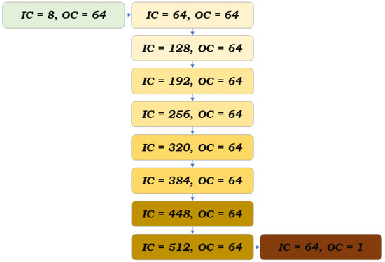
Figure 1.
The model architecture. Each rectangle represents a layer, and the two numbers indicate the number of input and the number of output channels. In each layer, there are two convolutional operations as in Equation (1). In the intermediate layers, each output is concatenated to the input of the same layer and is passed to the next layer.
The activation function, Equation (2) (see Figure 2), is applied to the outputs of the two convolution operators after they are concatenated before being passed to the next layer.
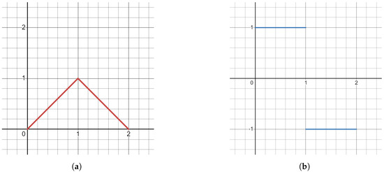
Figure 2.
The graph of the activation function (a) and the graph of its derivative (b).
The samples x and y of size , where N is arbitrary, are part of the input data for the model. We augment the input data with first-order, second-order, and third-order forward differences as presented in Equation (3).
The output of the model is a vector of probabilities, of length N, where the kth entry is the probability that there is a discontinuity between the kth and th sample. The loss function is cross-entropy [10] as the problem is classification.
Let be the model, and let . Then, is the index of the closest sample to the discontinuity point from the left side. We define
as the approximated discontinuity point.
2.2. Training Data
In this section, we outline the process of generating synthetic data for training the model, both as input and output. We recall that a random number between a and b from a uniform distribution is denoted as
We start by generating univariate piecewise functions, each containing a jump discontinuity, from which we randomly sample points. To create a realistic scenario, we introduce white noise to these samples and use them as input data. The output data consist of the index of the closest sample to the left side of the jump discontinuity. Let
be the set of knots where and , so there are enough knots inside and outside the interval, and let
Now, we let
Here, are cubic B-splines basis functions (k = 3). The coefficients of the cubic B-splines are selected randomly from a uniform distribution:
Similarly, the coefficients a and b are selected.
Finally, the location of the discontinuity point is as follows:
The input data consist of points sampled from a function of the form as in Equation (7):
where
Here, is the additive noise. The output is a unit vector of length where the 1 is located at the closet sample from the left of the jump discontinuity. We train the model with the ADAM [12] stochastic gradient descent algorithm.
2.3. Approximating the Function from Its Samples
After locating the discontinuity interval and approximating the discontinuity point’s location, we utilize two cubic spline approximations to approximate the function with its jump discontinuity. We use the cubic spline approximation because approximating with cubic splines is advantageous due to their smoothness, flexibility, accuracy, ease of implementation, and numerical stability. These properties make cubic splines a versatile and widely used tool for data interpolation, curve fitting, and modeling in various fields, including mathematics, engineering, computer graphics, and scientific computing [13].
First, we split the data into the left groups and the right groups as follows:
where is defined as in Equation (8) and is from Equation (5).
Then, by using a least squares approximation, we find two cubic splines, , which approximates the function from the left side of the jump discontinuity by using the data of and and second one, , which approximates the function from the right side of the jump discontinuity by using the data of and . Before proceeding, we begin by constructing the knots for both splines. Let
and let and . Then, the two sets of knots for the left and the right approximations are
We denote the set of the coefficients of and by and , respectively. To find the optimal sets of coefficients and , we find a closed-form solution for the following equation:
Here, the matrices of are the data matrices and are defined as follows:
The matrices of are the second difference matrices. Those matrices are used in the above equation so that the optimal solution is the one with a minimal second-derivative.
3. Numerical Results
In this section, we illustrate the two aspects of our approach: approximating the location of a jump discontinuity in a given function and approximating the function itself. Furthermore, we conducted a statistical test to show the effectiveness of our method compared to two alternative methods. Lastly, we performed another statistical test to present the average error of our final approximation.
3.1. Detecting the Interval of the Discontinuity and Approximating the Function
In this section, we present our approach to approximating the discontinuity point of a randomly generated function and subsequently approximating the function itself. To accomplish this, we generated two functions following the format described in Equation (7). We took 40 random samples from . These samples were then subjected to the addition of white noise with a variance equal to one-third of the jump’s height.
Next, we employed our model to determine the index of the closest sample from the left of the discontinuity. Subsequently, we utilized the procedure outlined in Section 2.3 to derive an approximation of the function. The results of these experiments are presented in Figure 3.
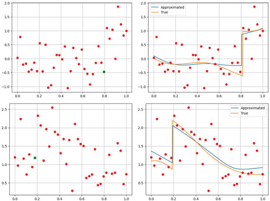
Figure 3.
We demonstrate our method visually by approximating the location of the discontinuity point of two univariate piecewise smooth functions from their samples, to which white noise was added. The upper-left and lower-left figures show the samples with the added noise. All samples are red-colored except for the point that indicates the closest sample from the right to the jump discontinuity, which is green-colored. Our approach found the green point. The upper-right and the lower-right figures show the approximations for the two functions, which were achieved using two cubic splines for each one of the functions.
3.2. Comparing Our Approach with Two Other Approaches
In [6], the signature, of degree k, of g, is , which is the forward kth-order difference of the samples of g padded by k zeros on each side. In [9], a method was developed based on the use of a filter function with which a convolution is computed for detecting the discontinuity point. In this experiment, we compare our method with the other two aforementioned methods on a large number of samples with various noise levels. The samples are taken from univariate piecewise smooth functions with several discontinuity jump heights. Table 1, Table 2 and Table 3 each represent the results of one of the approaches. The columns represent the height of the jump, and the rows represent the variance in the additive white noise. As shown in the tables, our approach has an increase of between twofold and tenfold compared to the other methods.

Table 1.
The probability of detecting the interval of the discontinuity location using the method in [6]. Columns and rows represent jump height and noise level, respectively. Each cell contains the average success of 1000 trials.

Table 2.
The probability of detecting the interval of the discontinuity location using the method in [9]. Columns and rows represent jump height and noise level, respectively. Each cell contains the average success of 1000 trials.

Table 3.
The probability of detecting the interval of the discontinuity location using our method. Columns and rows represent jump height and noise level, respectively. Each cell is the average success of 1000 trials.
3.3. Error Measurement of Approximations of Functions
In this experiment, we compare our approach with the approach of using the signature [6] in approximating a univariate piecewise smooth function from its noisy samples. As before, we ran a test on many samples with various noise levels. We measure the error of the approximation by using the metric on the set , where and are the real and the approximated point of discontinuity. Additionally, we measure . We created two graphs, in Figure 4 and Figure 5, for the two approaches and the two measurements. The x-axis represents the variance of the additive white noise, whereas the y axis represents the height of the jump. Each point in the graph represents the average error of 100 trials. In the first test, the error of our approach was less than half of the error of the other approach, and in the second test, the error of our approach was fifth.
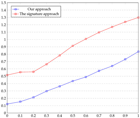
Figure 4.
This graph shows the -error of the approximation on the set , where and are the real and the approximated point of discontinuity. Here, and are the real and the approximated point of discontinuity.
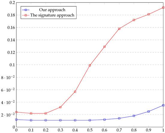
Figure 5.
This graph shows the error of . Here, and are the real and the approximated point of discontinuity.
4. Conclusions
We presented a new approach, which is based on deep learning, to approximate the location of the point of jump discontinuity from given samples, with highly additive noise, of a univariate piecewise smooth function with a jump discontinuity. We compared our approach against two other methods and illustrated the significantly higher success rate of our method against them. In addition, we demonstrated our approach to approximating the location of the discontinuity in synthetic data of generated piecewise smooth univariate functions. Then, we approximated these functions and showed the error measurements. Our future work will deal with extending this work to bivariate piecewise smooth functions, in which the jump does not occur at one point but rather on a one-dimensional curve. In case that the two-dimensional data are equally distanced along the y-axis, we can utilize this approach to locate the nearest points to the one-dimensional curve. However, approximating the one-dimensional curve is not intuitive and will be a subject for future work.
Author Contributions
Methodology, Q.M.; investigation, Q.M.; writing—original draft preparation, Q.M.; writing—review and editing, M.W. and Q.M.; supervision, M.W. and D.L. All authors have read and agreed to the published version of the manuscript.
Funding
ISF Israeli Science Foundation.
Data Availability Statement
There are no specific data used in this paper.
Conflicts of Interest
The authors declare no conflict of interest.
References
- Ageev, A.L.; Antonova, T.V. On a new class of ill-posed problems. Izv. Ural. Gos. Univ. Mat. Mekh. Inform. 2008, 58, 24–42. [Google Scholar]
- Cherepashchuk, A.M.; Goncharskii, A.V.; Yagola, A.G. Inverse problems of astrophysics. In Ill-Posed Problems in Natural Sciences, Proceedings of the International Conference Held in Moscow, August 19–25, 1991; De Gruyter: Berlin, Germany, 1992; pp. 472–481. [Google Scholar]
- Terebizh, V.Y. Introduction to the Statistical Theory of Inverse Problems; Fimzmatlit: Moscow, Russia, 2005. [Google Scholar]
- Aràndiga, F.; Donat, R. Nonlinear multiscale decompositions: The approach of A. Harten. Numer. Algorithm 2000, 23, 175–216. [Google Scholar] [CrossRef]
- Shu, C.-W. Essentially non-oscillatory and weighted essentially non-oscillatory schemes for hyperbolic conservation laws. In Advanced Numerical Approximation of Nonlinear Hyperbolic Equations: Lectures Given at the 2nd Session of the Centro Internazionale Matematico Estivo (C.I.M.E.) Held in Cetraro, Italy, June 23–28, 1997; Springer: Berlin/Heidelberg, Germany, 1998; pp. 325–432. [Google Scholar]
- Amat, S.; Levin, D.; Ruiz-Álvarez, J. A two-stage approximation strategy for piecewise smooth functions in two and three dimensions. IMA J. Numer. Anal. 2021, 42, 3330–3359. [Google Scholar] [CrossRef]
- Antonova, T.V. New methods for localizing discontinuities of a noisy function. Numer. Anal. Appl. 2010, 3, 306–316. [Google Scholar]
- Mbakop, E. Reconstruction of Discontinuities in Noisy Data; Citeseer: Pennsylvania, USA. Available online: https://citeseerx.ist.psu.edu/document?repid=rep1&type=pdf&doi=0c1b69c38e1df16c7c939ad07705ee6bb53a6bd2 (accessed on 31 March 2024).
- Lee, D. Detection, Classification, and Measurement of Discontinuities. SIAM J. Sci. Stat. Comput. 1991, 12, 311–341. [Google Scholar] [CrossRef]
- Goodfellow, I.; Bengio, Y.; Courville, A. Deep Learning; MIT Press: Cambridge, MA, USA, 2016. [Google Scholar]
- LeCun, Y.; Bengio, Y.; Hinton, G. Deep learning. Nature 2015, 521, 436–444. [Google Scholar] [CrossRef] [PubMed]
- Kingma, D.P.; Ba, J. Adam: A method for stochastic optimization. arXiv 2014, arXiv:1412.6980. [Google Scholar]
- Chapra, S.C.; Canale, R.P. Numerical Methods for Engineers, 8th ed.; McGraw-Hill Education: New York, NY, USA, 2021. [Google Scholar]
Disclaimer/Publisher’s Note: The statements, opinions and data contained in all publications are solely those of the individual author(s) and contributor(s) and not of MDPI and/or the editor(s). MDPI and/or the editor(s) disclaim responsibility for any injury to people or property resulting from any ideas, methods, instructions or products referred to in the content. |
© 2024 by the authors. Licensee MDPI, Basel, Switzerland. This article is an open access article distributed under the terms and conditions of the Creative Commons Attribution (CC BY) license (https://creativecommons.org/licenses/by/4.0/).