

NICE: A Web-Based Tool for the Characterization of Transient Noise in Gravitational Wave Detectors
by
 , , , and
Nunziato Sorrentino
1,2,*,†,
Massimiliano Razzano
1,2,†,
Francesco Di Renzo
3,
Francesco Fidecaro
1,2 and
Gary Hemming
4 1
Department of Physics, Università di Pisa, I-56127 Pisa, Italy
2
Sezione di Pisa, INFN, I-56127 Pisa, Italy
3
Université Lyon, Université Claude Bernard Lyon 1, CNRS, IP2I Lyon/IN2P3, UMR 5822, F-69622 Villeurbanne, France
4
European Gravitational Observatory (EGO), Cascina, I-56021 Pisa, Italy
*
Author to whom correspondence should be addressed.
†
These authors contributed equally to this work.
Software 2024, 3(2), 169-182; https://doi.org/10.3390/software3020008
Submission received: 26 January 2024
/
Revised: 12 April 2024
/
Accepted: 14 April 2024
/
Published: 18 April 2024
(This article belongs to the Topic Software Engineering and Applications)
Abstract
:NICE—Noise Interactive Catalogue Explorer—is a web service developed for rapid-qualitative glitch analysis in gravitational wave data. Glitches are transient noise events that can smother the gravitational wave signal in data recorded by gravitational wave interferometer detectors. NICE provides interactive graphical tools to support detector noise characterization activities, in particular, the analysis of glitches from past and current observing runs, passing from glitch population visualization to individual glitch characterization. The NICE back-end API consists of a multi-database structure that brings order to glitch metadata generated by external detector characterization tools so that such information can be easily requested by gravitational wave scientists. Another novelty introduced by NICE is the interactive front-end infrastructure focused on glitch instrumental and environmental origin investigation, which uses labels determined by their time–frequency morphology. The NICE domain is intended for integration with the Advanced Virgo, Advanced LIGO, and KAGRA characterization pipelines and it will interface with systematic classification activities related to the transient noise sources present in the Virgo detector.
Keywords:
gravitational wave; interferometer; web-application; LIGO; Virgo; KAGRA; detector characterization; glitch; noise1. Introduction
Advanced LIGO [1], Advanced Virgo [2], and KAGRA [3] are gravitational wave (GW) detectors developed as kilometers-long Michelson interferometers, with a complex optical and mechanical design used for reducing most environmental and experimental noise. GWs are linear perturbations of the space–time metric, as predicted by Einstein’s field equations, and were discovered in 2016 by the LIGO and Virgo scientists in the form of a binary black hole coalescence signal [4]. This event was named GW150914 and was detected during the first observing run, named O1, using data from the two Advanced LIGO interferometers, thus opening the era of GW astronomy. During the second observing run (O2) there were other important milestones such as the first three-interferometer detection (GW170814) with Advanced Virgo [5] and the first multi-messenger observation of a merging binary neutron star system (GW170817) [6,7,8].
From April 2019 to March 2020, during the third observing run (O3, subsequently divided into O3a and O3b), which included Advanced LIGO, Advanced Virgo, and (for the last days of the run) KAGRA, the rate of identification of GW candidates grew significantly, reaching a total of 93 GW events confirmed as compact binary coalescences [9,10,11,12]. GW signal detection is the result of a complex analysis that extracts GW signals from a continuous noise signal originating from different sources. Many of these sources are the result of stochastic processes that can be modeled to be stationary and Gaussian [1,2,3]. There are also both non-stationary and non-Gaussian noise artifacts, which can be transient or persistent in the detector, whose presence affects the data quality of the “strain channel” (where the passage of GW is recorded) [13].
The analysis of GW signals deals with non-Gaussian transient noise sources of instrumental or environmental origin, known as “glitches”, that reduce the significance of signal detection and introduce systematic errors in the estimate of astrophysical source parameters [14]. The glitch rate is much higher than the GW event rate and many glitches can mimic the presence of transient GWs [15], thus increasing the probability of a false alarm [10,11,14]. Therefore, studying glitches is a crucial point for characterizing a detector and increasing its sensitivity.
Most glitch studies are based on characterization in the time–frequency domain. Glitches are usually detected through algorithms named event trigger generators (ETGs), such as Omicron [16]. ETGs exploit various methods to detect transient events, e.g., excess power, and produce metadata describing glitches, such as peak time or frequency range [17]. Omicron is used also for time correlation studies (see Section 5 for details) and includes both the strain channel and the data from environmental and instrumental sensors, which are located all around the experimental apparatus and are known as “auxiliary channels”. This study is carried out to understand the coupling mechanism at glitch origin.
In addition to correlation studies, glitches can be also identified with time–frequency patterns presented in spectrograms or Q-scans. These are the results of the Q-transform application, which leads to a rapid visualization of a transient event, characterizing it from a morphological point of view [18,19]. The Q-transform produces a multi-resolution time–frequency map of the noise excess, based on a transform whose resolution can be parameterized using a quality factor , where is the central frequency and the bandwidth. For more information see [20].
Glitch morphology identification is called “classification” and helps understand the origin of a glitch population that presents common time–frequency patterns, often found recurrent in some auxiliary channels.
In GW detector characterization, it is important to return a quick response during the validation of a trigger, which consists of evaluating if there is the presence of a glitch nearby a transient GW signal event candidate [10]. Alerts related to candidate GW events are sent to astronomers for potential electromagnetic follow-up.
The possibility to perform a rapid and interactive analysis of glitches is important in the analysis of transient GW signals, whose rate is growing with the improvement in advanced detector sensitivity. Web-based systems designed to monitor the status of the various subsystems of the detector, as well as environmental conditions, are systematically used for these detector characterization activities [21,22]. However, to date, in the Virgo and LIGO collaboration, there is no dedicated web-based tool specifically designed to perform a quick-look analysis of glitches. We have developed the Noise Interactive Catalogue Explorer (NICE) in this context. This is a web interface with a back-end database containing the glitch information found by ETGs. NICE provides a dynamic on-demand computing environment, a user-controllable view of data, and quick-look analysis tools for glitches. It allows us to easily visualize glitch rates for different glitch populations, suitable for detector characterization and noise-hunting activities. NICE also allows the visualization of the classification information for each glitch (called “class label”), allowing scientists to study and compare glitches of the same morphology, as well as study morphology in the strain channel and compare that with that of glitches in auxiliary channels. Class labels and high interactivity represent some of the main innovations among other web-based monitors. NICE has been developed to facilitate the work of scientists, presenting them with an end-to-end workflow to solve problems related to noise contamination. Since there are still ongoing citizen science projects for glitch classification, and since NICE was developed post-O3, the software does not contain classified glitches and is not already used for vetting GW event candidates. For these reasons, its functionality and its impact on detector characterization are shown here taking into account strain data with simulated glitches and their relative classification labels.
The rest of this work is divided into the following sections. In Section 2, there is a summary of the related tools used to monitor GW detector noise and how NICE proposes to overcome their limits. In Section 3, there is a detailed description of the software architecture and workflow, with a particular focus on event validation use cases. In Section 4, there is an example application on simulated glitches that are common in the Virgo detector. Section 5 contains the impact of this tool on the detector characterization done with the pipelines available to LIGO, Virgo, and KAGRA members, together with the integration proposed for class labels coming from citizen science activities. Section 6 contains a brief discussion of NICE application and structural limits and how authors foresee overcoming these. Finally, Section 7 presents the conclusion regarding this new technology alongside possible future applications.
2. Related Work
The NICE web service is proposed as a new integration to the monitoring system of Virgo detector noise. There are various analysis tools for monitoring the Virgo detector as follows [23]:
- The dataDisplay: software that allows users to read Virgo data from all available channels and visualize various types of plots for detector characterization (e.g., spectrograms or coherence tests) [24];
All these tools offer a graphic interface to easily manage and analyze data quality, but only the third one contains a script specific to glitches. Furthermore, such graphical interfaces do not allow interactive editing of plots and tables, which are saved as static images in a database, and have access to glitch metadata that does not include classification labels.
For LIGO detectors, there is still a wide range of tools used to monitor data quality and characterize the detectors [27,28,29], incorporating also the classification labels of a dedicated citizen science project [30].
NICE proposes to fill these gaps within the Virgo noise analysis chain and presents software within an interactive graphic interface, which is described in Section 3.
3. Software Description
The NICE v1 software provides interactive graphical plots for the study of glitch populations and data analysis tools for the origin and morphology investigation of a single glitch component. In this Section, the software components (Section 3.1), along with the most frequent cases of interest for detector characterization (Section 3.2), are described.
3.1. The Tool’s Architecture
The NICE architecture is illustrated in Figure 1. Its interface communicates with a multiple-database infrastructure, which we will refer to as “GlitchDB”, specifically designed to store the metadata for a high number of glitches recorded in the GW data from the O2 run onward. To date, the database contains metadata about glitches calculated by Omicron on Virgo strain and auxiliary channels (see Section 3.1.1 for more details) [17]. The NICE interface presents a Homepage shown in Figure 2, which allows two investigation approaches to users. The first investigation approach returns glitch metadata in a table format and is carried out through the Search button. The second approach to making a glitch request is through the Plot button. This opens the Interactive Plot Window (IPW), which is a tool dedicated to the visualization of the distribution of glitches around a reference time (see Section 3.1.3 for more details). Clicking on a single peak time of the glitch table obtained with the Search button, or similarly, on the glitch scatter point of the IPW graph, it is possible to access the Single Glitch Analysis Window (SGAW), which uses strain and auxiliary data for the single glitch analysis (see Section 3.1.4 for more details).
3.1.1. Database Infrastructure for Glitches
The GlitchDB is the back-end component of NICE. It consists of multiple storage units, illustrated in Figure 1. GlitchDB is built and managed with pymysql 0.9.3 modules [31] and was made to support foreign-key references and null table elements. Its creation was necessary to enable the use of a single structure for the storage of all glitches affecting the detectors, which reaches ∼ triggers for each observing run (as counted by NICE). The metadata stored in it is freely accessible to LIGO, Virgo, and KAGRA members. GlitchDB comprises one database per observing run, used as archives in high-latency servers. In addition, one database is available for periodic uploads of real-time glitch metadata and will be devoted to the next runs’ detector characterization stages. This multi-database organization has been set up to optimize the request stage, given that a median glitch rate of ∼1 trigger per minute was archived in a single strain channel during O3b [11]. We chose this database organization for retrieving both the archived glitch metadata and the ongoing glitch information generated in the current observing run within a single request unit. Indeed, ETGs like Omicron generate metadata that is not located on the same server during the different runs. For this reason, this project needed to create a new memory unit containing the full history of ETG triggers.
Omicron has been chosen as the ETG for this project for its low-latency results, which are easily converted for integration into the GlitchDB architecture. For future detector runs, NICE will be automatically filled with Omicron low-latency results using the cron-job (cron-job.org: https://cron-job.org/en/, accessed on 12 April 2024) utility. Thanks to its flexibility, GlitchDB is ready to host other metadata generated by other ETGs, such as the triggers from PyCBC [32].
3.1.2. Glitch Request Page
According to the user analysis goal, it is possible to send queries to GlitchDB by clicking on both the Search and Plot buttons and passing the following glitch parameters:
- GPS-time (all data are stored in the GPS time system, which is the number of seconds from 00:00 of 6 January 1980) interval;
- Central frequency range;
- Minimum and maximum signal-to-noise ratio (SNR) values;
- ETG name(s) that generated the glitch’s metadata;
- Channel name(s), i.e., the LIGO–Virgo–KAGRA strain channels and/or the most interesting auxiliary channels, which are usually called “first-look channels”;
- Class label(s) and/or select glitches that are not classified in the database.
Glitch SNR is defined here as the amplitude of the Q-transform coefficients of the whitened data (there is more information in [16,17]). Then, the first-look channels are chosen for checking the most common culprits related to the presence of glitches, e.g., a sudden excess of noise or exponential increment of a triggers population. When studying the population of glitches, it is important to classify them in a set of finite labels. These labels are based on the knowledge of already identified glitches and their names are based on their physical origin or, when this is not known, on their morphology as visible from the Q-transform application. A list of labels and images of different glitch typologies can be found in the dataset of the Gravity Spy citizen science project [33]. Here, glitches with the Koi Fish label, for example, are characterized by a head at the low frequencies of the Q-scan, fins at around 30 Hz, and a thin tail at around 500 Hz [34]. Conversely, there is the Scattered Light label, which describes one or multiple low-frequency and long-duration arcs. These glitches are correlated with different mechanisms of light scattered into the interferometer’s arms [34,35]. The Scattered Light glitch is one of the examples explored in Section 4.
Once the glitch metadata are obtained from the GlitchDB query, it is possible to then download the selected glitches in CSV format (Search button) or switch to the graphical tools provided by IPW and SGAW (Plot button), where the NICE proper tools for glitch visualization and quick-look analysis are contained.
3.1.3. Interactive Plot Window (IPW)
In the IPW, the user can explore the distribution of glitch properties in the detector through a graphical interactive tool. In particular, there are three different plots by which it is possible to customize display parameters, e.g., by zooming in on particular regions of the plots or to choose which glitch parameters to plot. Thanks to the Bokeh 2.0.2 library [36], the axes values can be chosen from all requested glitch properties (e.g., peak time, frequency, and SNR), which are further selectable within the relative widgets.
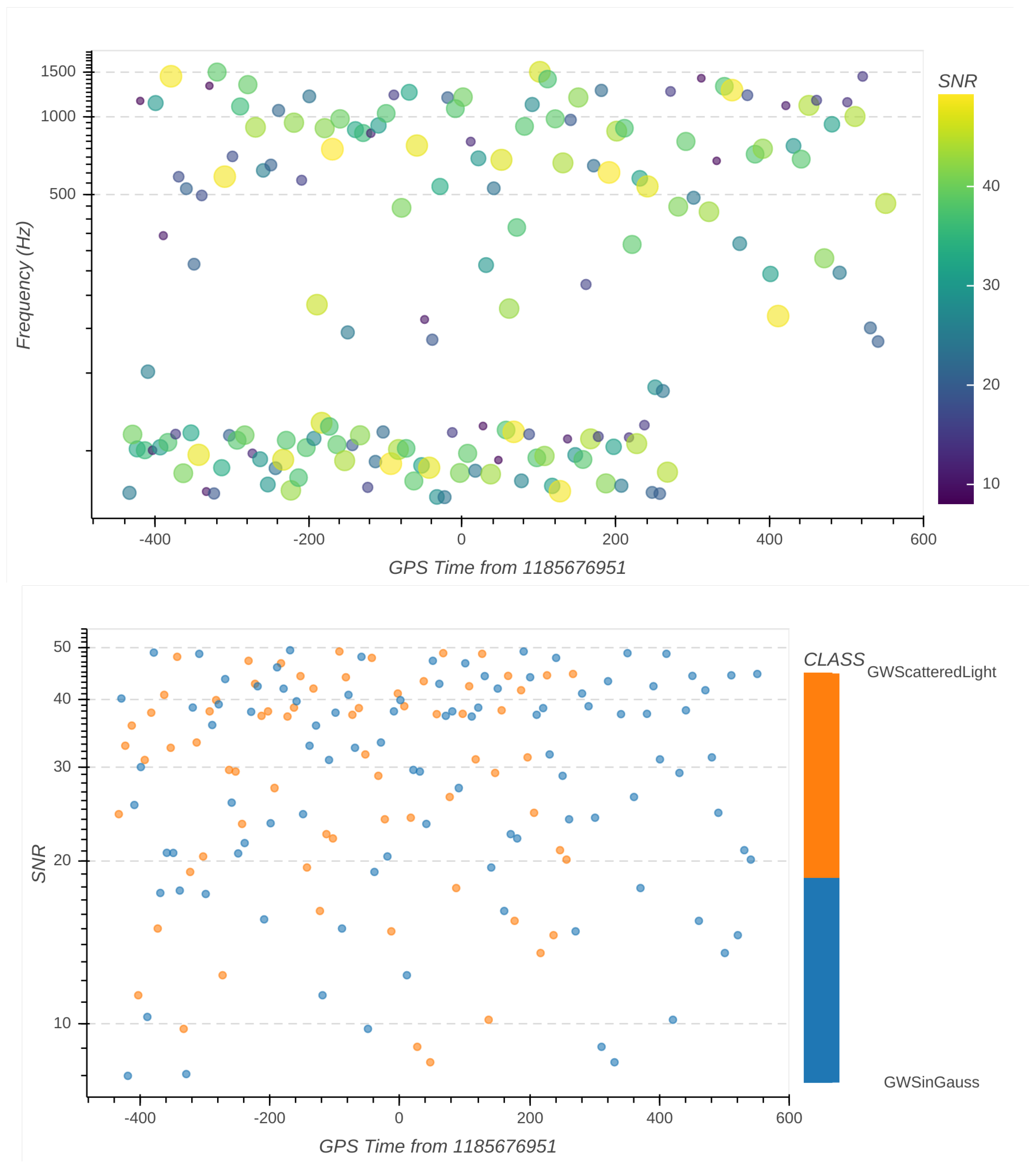
The first plot is a 2D distribution (see Figure 3) and can be customized using the widgets dedicated to channel and ETG selection. A third widget transforms the color and the shape of the points according to the bar values, whose ticks can be chosen between SNR values and glitch labels. The last two plots are 1D histograms containing the count distribution synchronized with the 2D graph axes (see Figure 4).
These three plots can be saved and the figures can be managed with the graphical toolbar below, which allows the user to zoom into the images and/or select a subset of data for closer investigation.
3.1.4. Single Glitch Analysis Window (SGAW)
The SGAW contains functions that read and process data from strain and auxiliary channels around the time of a glitch. That is carried out using gwdama 0.5.3 (GwDama software documentation: https://gwnoisehunt.gitlab.io/gwdama/, accessed on 12 April 2024), a Python library specifically developed for GW data processing. Meanwhile, the Q-transform used for the glitch morphology calculation is obtained through the algorithm implemented in the gwpy 1.0.1 library [37].
As mentioned in Section 3.1, the SGAW tools are made accessible by clicking on each glitch point in the IPW main plot. Data from LIGO–Virgo–KAGRA strain channels and Virgo auxiliary channels are provided to several online processes at the Virgo site, where data are stored for ∼6 months [2], and are used by SGAW for the analysis carried out during the current observing run. Then, the data are transferred to computing centers for offline analysis and, from this point forward, SGAW uses just the strain channels of the Virgo detector located at the detector site for the offline analysis. Finally, NICE stores the glitch metadata generated by Omicron during the run that has just finished.
SGAW shows a summary of the information available about a single glitch, e.g., the name of the ETG that generated it and the corresponding description. It also contains an explanation of how the glitch has been classified and provides the following four main features for a deeper analysis of the event:
- Overview: shows the name and the description of the label used to classify the glitch;
- Coincident Channels: allows the origin of a glitch to be investigated and the listing of all glitches whose peaks are time-coincident across the strain channel and the first-look auxiliary channels, providing the name of the ETG that generated that trigger and the details of the glitch given by the ETG itself. Here, the user can download a table with the metadata and compute a Q-scan of the glitch in the strain and auxiliary channels where coincident peaks of energy are present;
- Download: a download button, which allows the user to download 1 min of strain data around the time of a glitch;
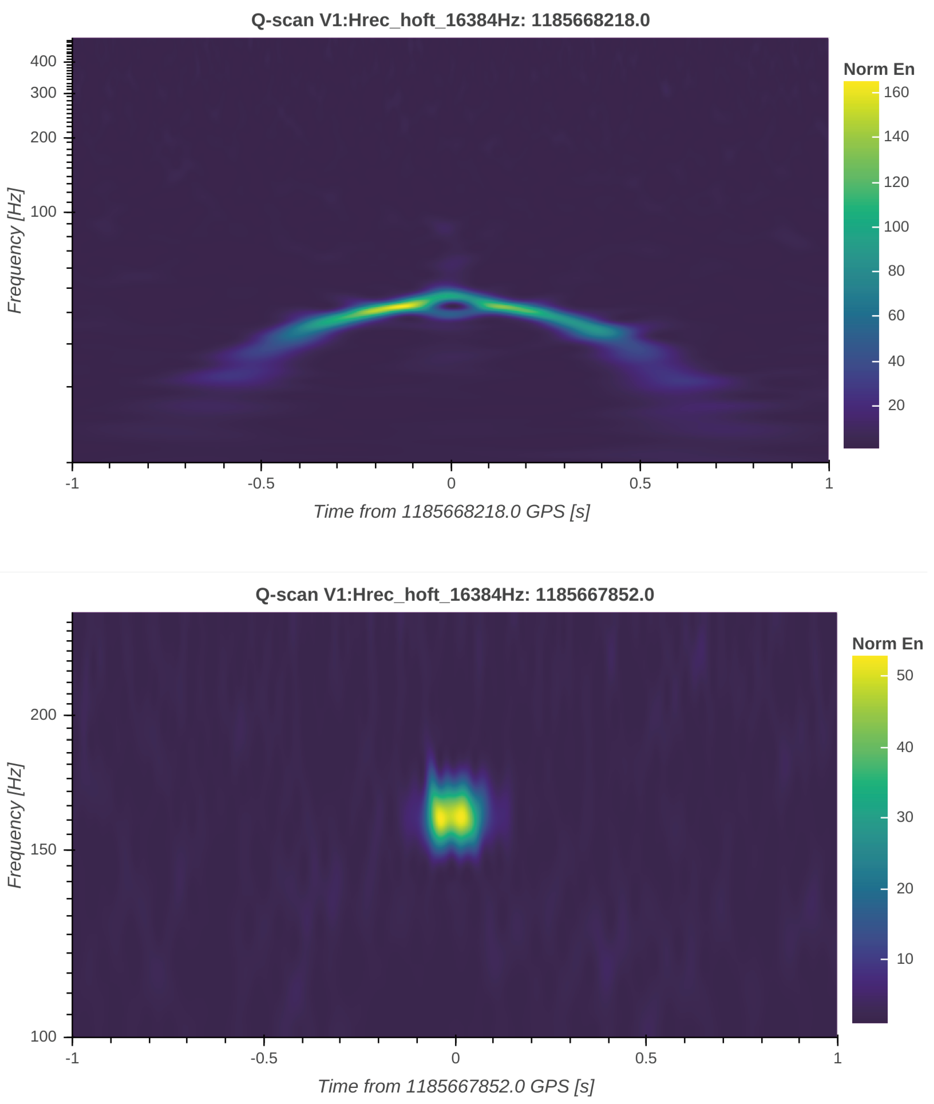
- Visualization: as with the second section, data are read and transformed for morphology visualization, which contains the necessary patterns for the classification (see Figure 5 for the example carried out with simulated strain data). Additionally, the time window around the trigger can be set to fit with the glitch duration. A toolbar is present below that makes it possible to save the result, move the time–frequency position, and zoom in on the glitch component.
3.2. The Tool’s Functionalities
The Search and Plot buttons open the interfaces that must be used for sending a request to GlitchDB. These allow users to obtain glitch metadata in the desired format, e.g., the interactive plots provided by IPW. From the IPW, it is possible to access SGAW functionalities with a simple double-click method, passing from a glitch population visualization to a single glitch characterization. This link between IPW and SGAW was developed to facilitate the plotting and analysis of single glitches as well as glitch populations.
The IPW plots are particularly useful in obtaining the glitch rate around a GW candidate event (see Figure 3 and Figure 4). For instance, the IPW can show how many glitches are present around a time, their SNRs, and whether the glitches are classified and, if so, with which label (see Figure 3). The additional possibility of changing the values associated with the plot axis (e.g., the change from frequency to SNR on the y-axes of the plots in Figure 3) and the possibility of investigating both past and current observing runs make this tool ideal for understanding whether a glitch class distribution has already been observed (see Section 5 for details).
The SGAW functionalities are dedicated to the quick-look characterization of the single glitch. This can be done by comparing the list of coincident triggers from a set of auxiliary channels that can be selected by the user and performing a Q-transform. This is useful when searching for the possible cause of a glitch and looking at similar power excesses in the strain and auxiliary channels. The possibility of downloading strain data around the glitch time has been provided to permit dedicated offline investigations with user-made analysis tools. The Q-transform performed on the strain data channel also helps scientists identify glitches that have a particular time–frequency morphology but do not have a classification label yet (see Figure 5). This makes the SGAW tool a good collector of ideas for the possible classifications of these glitches. Making use of these web-based functionalities leads to a fast and effective tool for managing information about the glitch rate, calculated as in Figure 4. Note that NICE provides also the possibility of making a class query to GlitchDB, thus showing the glitch rate of a particular family around the trigger of a GW candidate. Is the glitch already classified with a particular label, thus rendering unlikely a potential astrophysical origin? If it is so, the glitch morphology can be visualized for assessing a first discrimination decision and then analyzed with a quantitative tool external to NICE (see Section 5).
4. Description of the Tool’s Operation
An example of the distributions provided by NICE is shown in Figure 3 and Figure 4. These show a dataset of ∼1000 s of simulated glitches, uniformly distributed in time and injected into simulated white noise. To show the capability of NICE to deal with glitches on different time scales, we use here two classes of glitches, sin-Gaussian and Scattered Light. The former are short-lived glitches, while the latter last for a few seconds and are associated with scattered light in the mirrors of the detectors.
The GWSinGauss family of glitches is characterized by a sine wave modulated by a Gaussian function, the amplitude of which is [38]:
where is the strain amplitude, and are the central time and frequency of the glitch, and is its characteristic duration.
The GWScatteredLight family represents a common low-frequency noise in a GW detector and is due to the propagation of scattered light through the various sub-systems of the detector [39]. These glitches appear as a series of arcs that can last up to ∼1 s and their can be modeled using the formula [38]:
where is:
and K is a “curvature” parameter set to to mimic a subset of arcs due to the scattered light like the one shown in Figure 3 in [35].
In Table 1, we show the parameter ranges used in simulating the glitches, the uniform distribution in time of which is illustrated in Figure 3, using the results of IPW. Figure 4 shows the 1D histograms of glitch frequencies and GPS times that can be useful to determine the presence of clusters of glitches with similar properties
Figure 5 shows the SGAW output, obtained by calculating the Q-transform with the gwpy library [37], highlighting two peculiarities. First, both glitch morphologies are different from a chirp-like signal, which is typically produced by the merger of compact binary objects [4,6]. Furthermore, the arc due to scattered light is visible and the sin-Gaussian model fits with glitch symmetry around the center of the image. This morphological analysis is useful when comparing similar signals between strain and auxiliary channels, as well as when comparing glitches of the same family that present different peculiarities.
5. Impact on Detector Characterization
The impact of NICE on detector characterization activities arises from having a great versatility of usage, together with a varied set of glitch information, and being fast and easy to use. At the Virgo site, the online and offline detector characterization is done with the following dedicated tools:
- Used Percentage Veto (UPV) algorithm, which makes a statistical correlation between transient events in the strain channel and some auxiliary channels [40];
- Omicron itself, which can also perform a time-coincident trigger search between the strain channel and some auxiliary channels (Omicron documentation: https://virgo.docs.ligo.org/virgoapp/Omicron/, accessed on 12 April 2024).
With the NICE interactive tools IPW and SGAW, it is possible to modify the search, the analysis, and the plotting parameters according to the user’s purpose. It is also possible to obtain already classified glitch labels, which adds an important characteristic to the glitch distribution, if compared with the count rate and the loudness in a certain time interval, also obtained using the VIM interface.
The possibility with NICE of carrying out a Q-scan comparison across different data channels results in an efficient way of providing the auxiliary channels correlated with the strain channel, which can be used for further quantitative analysis. For example, a quick-look glitch correlation, obtained rapidly with SGAW functions, can be confirmed by estimating the correlation factor between the channels individuated by SGAW. Then, the correlation factor can be calculated by applying the UPV to the time interval around the glitch, or even with the LIGO hierarchical veto algorithm [41], which provides a different time correlation method concerning UPV.
NICE also proves to be very useful for inspecting long stretches of data (e.g., over one day), integrating a dynamic plotting ability, and the archived classifications labels, with the VIM information about glitches.
Since NICE keeps track of glitches detected in both past and current runs, its direct overview of the distribution plots also allows for a comparison with similar events that occurred in the past.
Different kinds of glitch families may evolve in different ways simply because of environmental conditions, operational conditions of the detector, or improvement in tracking the relative motion between the mirrors [10,11,42]. It is, therefore, important to have a tool that archives as much information as possible about glitches, whose metadata is well documented and handy to plot, and that allows for easy switching between single- and multiple-glitch investigation.
GlitchDB can host class labels produced by dedicated deep learning automatic classification pipelines [33,34,38] and citizen science projects such as Gravity Spy (Gravity Spy—Zooniverse: https://www.zooniverse.org/projects/zooniverse/gravity-spy, accessed on 12 April 2024) [33] and GWitchHunters (GWitchHunters Project: https://www.zooniverse.org/projects/reinforce/gwitchhunters, accessed on 12 April 2024) [43]. Many machine learning algorithms collect glitch metadata, see [44] for an exhaustive summary, using just the strain channel or adopting also data from the main auxiliary channels. These pipelines do not include a citizen science classification stage, as opposed to the Gravity Spy and GWitchHunters projects. Thanks to citizen science, we have a high number of samples for the glitch classification done using supervised learning algorithms, providing such labels during the detector characterization activities. In particular, the GWitchHunters project is currently collecting class labels from Virgo glitches affecting data during past runs. The aim is to create the dataset necessary for training deep learning classification pipelines, whose results will be collected and visualized by NICE, together with the training dataset [43].
A key aspect of NICE is its modularity. Its back-end MySQL database service allows for particular flexibility. It uses a database schema that allows for the integration of other kinds of noise sources that are present in the detectors, e.g., spectral lines [45]. It would be interesting to explore the versatility of graphical interaction by adding metadata about the wandering spectral lines that, in turn, contribute to the creation of false GW signals [34].
6. Threats to Validity
The NICE workflow is tested using real Omicron metadata from the O2 and O3 runs, previously archived in offline servers, and simulated noise data generated with two canonical glitch models. Based on these tests, we can identify some threats to the validity of this tool. Since it is not tested on real strain and auxiliary data, plots generated with SGAW may not be obtained in a reasonable latency for analysis purposes. Furthermore, some auxiliary channels may be inaccessible around the time of an Omicron glitch, and this possibility must be considered in the future development of NICE. With the hope of being able to carry out some tests during a run in progress, it is desirable to carry out the following:
- Compare plots obtained from VIM and NICE and check if Omicron glitch distribution plots are equal for those metadata updated every 24 h in the GlitchDB;
- Measure the speed with which plots are obtained from SGAW when having access to real data;
- Ensure there is a machine learning pipeline capable of providing glitch labels and uploading them to the database in a few seconds, to be able to use NICE also for the low-latency analysis of the detector status.
In the way that it was conceived, developed, and tested, NICE is designed to provide a quick-look analysis and must be considered as only a starting point for GW noise hunting, the results of which must be subsequently proved quantitatively with the tools mentioned in Section 5.
7. Conclusions
NICE is an interactive web-based service devoted to noise investigation in GW interferometers. During the commissioning period between the O3 and O4 runs, the software was tested on Advanced Virgo data and prepared for interfacing with Advanced LIGO and KAGRA data. We have shown that the approach proposed by NICE can be useful for detector characterization and GW event validation, and it can achieve this by utilizing different interactive quick-look analysis tools. Tools developed for monitoring the glitching status of the detector, e.g., VIM, already provide glitch distributions and single glitch morphology plots through static graphics, generated every day of a run. Differently from such related monitoring tools, NICE is intended for specific glitch analysis and introduces user interactivity and glitch class labels into a web-based GW system designed to monitor the glitching status of the detector. This software is ready for use during future observing runs, where GW events are expected to be more frequent than before. Future improvements to the NICE infrastructure include the use, during strain data collection, of low-latency glitch metadata and the use of other ETGs in addition to Omicron. Other classification labels will be integrated by NICE from the citizen science campaign carried out by the GWitchHunters project. NICE interactivity with glitch visualization will allow an easy investigation of the origin of these transient noise sources, thus mitigating the impact that glitches have on the detection of astrophysical signals.
Author Contributions
Conceptualization, N.S. and M.R.; methodology, N.S. and M.R.; software, N.S. and M.R.; validation, N.S.; formal analysis, N.S. and F.D.R.; investigation, N.S.; resources, G.H.; data curation, N.S. and F.D.R.; writing—original draft preparation, N.S.; writing—review and editing, N.S., M.R., F.D.R. and G.H.; visualization, N.S., M.R., F.D.R., F.F. and G.H.; supervision, N.S, M.R., F.D.R. and F.F.; project administration, M.R. and F.F.; funding acquisition, M.R., F.F. and G.H. All authors have read and agreed to the published version of the manuscript.
Funding
This research was funded by European Union’s Horizon 2020 research and innovation program, under REINFORCE, grant number 872859.
Institutional Review Board Statement
Not applicable.
Informed Consent Statement
Not applicable.
Data Availability Statement
The simulations and the NICE package are made available in open-source format at the following link: https://github.com/nunziosorrentino/nice (accessed on 12 April 2024). For more information on how to prepare NICE locally and be able to demonstrate it with simulated data, consult https://nice-doc.readthedocs.io/en/latest/?badge=latest (accessed on 12 April 2024). The NICE v1 software presented here refers to the one used during the software staging phase, carried out during the commissioning period between the O3 and O4 runs.
Acknowledgments
This software has made use of the computing resources of the European Gravitational Observatory (EGO). For this reason, the authors want to thank Giuseppe Di Biase for their help in the materialization of the project and in making it available to collaboration members. The LIGO observatory is funded by the United States National Science Foundation (NSF), the Science and Technology Facilities Council (STFC) of the United Kingdom, the Max Planck Society (MPS), and the State of Niedersachsen (Germany). Virgo is funded by EGO, the French Centre National de Recherche Scientifique (CNRS), the Italian Istituto Nazionale della Fisica Nucleare (INFN), and the Dutch Nikhef.
Conflicts of Interest
The authors declare no conflict of interest.
Abbreviations
The following abbreviations are used in this manuscript:
| NICE | Noise Interactive Catalogue Explorer |
| GW | Gravitational Wave |
| ETG | Event Trigger Generator |
| GlitchDB | Glitch Database |
| SNR | Signal-to-Noise Ratio |
| IPW | Interactive Plot Window |
| SGAW | Single Glitch Analysis Window |
| VIM | Virgo Interferometer Monitor |
| UPV | Used Percentile Veto |
References
- Aasi, J.; Abbott, B.P.; Abbott, R.; Abbott, T.; Abernathy, M.R.; Ackley, K.; Adams, C.; Adams, T.; Addesso, P.; Adhikari, R.X.; et al. Advanced LIGO. Class. Quantum Grav. 2015, 32, 074001. [Google Scholar] [CrossRef]
- Acernese, F.; Agathos, M.; Agatsuma, K.; Aisa, D.; Allemandou, N.; Allocca, A.; Amarni, J.; Astone, P.; Balestri, G.; Ballardin, G.; et al. Advanced Virgo: A second-generation interferometric gravitational wave detector. Class. Quantum Grav. 2015, 32, 024001. [Google Scholar] [CrossRef]
- Aso, Y.; Michimura, Y.; Somiya, K.; Ando, M.; Miyakawa, O.; Sekiguchi, T.; Tatsumi, D.; Yamamoto, H. Interferometer design of the KAGRA gravitational wave detector. Phys. Rev. D 2013, 88, 043007. [Google Scholar] [CrossRef]
- Abbott, B.P.; Abbott, R.; Abbott, T.D.; Abernathy, M.R.; Acernese, F.; Ackley, K.; Adams, C.; Adams, T.; Addesso, P.; Adhikari, R.; et al. Observation of Gravitational Waves from a Binary Black Hole Merger. Phys. Rev. Lett. 2016, 116, 061102. [Google Scholar] [CrossRef] [PubMed]
- Abbott, B.P.; Abbott, R.; Abbott, T.D.; Acernese, F.; Ackley, K.; Adams, C.; Adams, T.; Addesso, P.; Adhikari, R.X.; Adya, V.B.; et al. GW170814: A Three-Detector Observation of Gravitational Waves from a Binary Black Hole Coalescence. Phys. Rev. Lett. 2017, 119, 141101. [Google Scholar] [CrossRef]
- Abbott, B.P.; Abbott, R.; Abbott, T.D.; Acernese, F.; Ackley, K.; Adams, C.; Adams, T.; Addesso, P.; Adhikari, R.X.; Adya, V.B.; et al. GW170817: Observation of Gravitational Waves from a Binary Neutron Star Inspiral. Phys. Rev. Lett. 2017, 119, 161101. [Google Scholar] [CrossRef] [PubMed]
- Abbott, B.P.; Abbott, R.; Abbott, T.D.; Acernese, F.; Ackley, K.; Adams, C.; Adams, T.; Addesso, P.; Adhikari, R.X.; Adya, V.B.; et al. Multi-messenger Observations of a Binary Neutron Star Merger. Astrophys. J. Lett. 2017, 848, L12. [Google Scholar] [CrossRef]
- Abbott, B.P.; Abbott, R.; Abbott, T.D.; Acernese, F.; Ackley, K.; Adams, C.; Adams, T.; Addesso, P.; Adhikari, R.X.; Adya, V.B.; et al. Gravitational Waves and Gamma-rays from a Binary Neutron Star Merger: GW170817 and GRB 170817A. Astrophys. J. Lett. 2017, 848, L13. [Google Scholar] [CrossRef]
- Abbott, B.P.; Abbott, R.; Abbott, T.D.; Abraham, S.; Acernese, F.; Ackley, K.; Adams, C.; Adhikari, R.X.; Adya, V.B.; Affeldt, C.; et al. GWTC-1: A Gravitational-Wave Transient Catalog of Compact Binary Mergers Observed by LIGO and Virgo during the First and Second Observing Runs. Phys. Rev. X 2019, 9, 031040. [Google Scholar] [CrossRef]
- Abbott, R.; Abbott, T.D.; Abraham, S.; Acernese, F.; Ackley, K.; Adams, A.; Adams, C.; Adhikari, R.X.; Adya, V.B.; Affeldt, C.; et al. GWTC-2: Compact Binary Coalescences Observed by LIGO and Virgo during the First Half of the Third Observing Run. Phys. Rev. X 2021, 11, 021053. [Google Scholar] [CrossRef]
- Abbott, R.; Abbott, T.D.; Acernese, F.; Ackley, K.; Adams, C.; Adhikari, N.; Adhikari, R.X.; Adya, V.B.; Affeldt, C.; Agarwal, D. GWTC-3: Compact Binary Coalescences Observed by LIGO and Virgo During the Second Part of the Third Observing Run. arXiv 2021, arXiv:2111.03606. [Google Scholar] [CrossRef]
- Abbott, R.; Abbott, T.D.; Acernese, F.; Ackley, K.; Adams, C.; Adhikari, N.; Adhikari, R.X.; Adya, V.B.; Affeldt, C.; Agarwal, D. GWTC-2.1: Deep Extended Catalog of Compact Binary Coalescences Observed by LIGO and Virgo During the First Half of the Third Observing Run. arXiv 2022, arXiv:2108.01045. [Google Scholar] [CrossRef]
- Abbott, B.P.; Abbott, R.; Abbott, T.D.; Abernathy, M.R.; Acernese, F.; Ackley, K.; Adamo, M.; Adams, C.; Adams, T.; Addesso, P.; et al. Characterization of transient noise in Advanced LIGO relevant to gravitational wave signal GW150914. Class. Quantum Grav. 2016, 33, 134001. [Google Scholar] [CrossRef] [PubMed]
- Abbott, B.P.; Abbott, R.; Abbott, T.D.; Abraham, S.; Acernese, F.; Ackley, K.; Adams, C.; Adya, V.B.; Affeldt, C.; Agathos, M.; et al. A guide to LIGO–Virgo detector noise and extraction of transient gravitational-wave signals. Class. Quantum Gravity 2020, 37, 055002. [Google Scholar] [CrossRef]
- Davis, D.; White, L.V.; Saulson, P.R. Utilizing aLIGO glitch classifications to validate gravitational-wave candidates. Class. Quantum Gravity 2020, 37, 145001. [Google Scholar] [CrossRef]
- Robinet, F. Omicron: An Algorithm to Detect and Characterize Transient Events in Gravitational-Wave Detector; Technical Report, VIR-0545C-14; Virgo TDS: Cascina, PI, Italy, 2018; Available online: https://tds.virgo-gw.eu/ql/?c=10651 (accessed on 12 April 2024).
- Robinet, F.; Arnaud, N.; Leroy, N.; Lundgren, A.; Macleod, D.; McIver, J. Omicron: A tool to characterize transient noise in gravitational-wave detectors. SoftwareX 2020, 12, 100620. [Google Scholar] [CrossRef]
- Brown, J. Calculation of a constant Q spectral transform. J. Acoust. Soc. Am. 1991, 89, 425–434. [Google Scholar] [CrossRef]
- Chatterji, S.K. The Search for Gravitational Wave Bursts in Data from the Second LIGO Science Run. Ph.D. Thesis, Massachusetts Institute of Technology, Department of Physics, Cambridge, MA, USA, 2005. [Google Scholar]
- Chatterji, S.; Blackburn, L.; Martin, G.; Katsavounidis, E. Multiresolution techniques for the detection of gravitational-wave bursts. Class. Quantum Gravity 2004, 21, S1809–S1818. [Google Scholar] [CrossRef]
- Berni, F.; Carbognani, F.; Dattilo, V.; Gherardini, V.; Hemming, G.; Verkindt, D. The Detector Monitoring System; Technical Report, VIR-0191A-12; Virgo TDS: Cascina, PI, Italy, 2012; Available online: https://tds.virgo-gw.eu/ql/?c=9005 (accessed on 12 April 2024).
- Berni, F. DMS Help Manual; Technical Report, VIR-0346A-20; Virgo TDS: Cascina, PI, Italy, 2020; Available online: https://tds.virgo-gw.eu/ql/?c=15469 (accessed on 12 April 2024).
- Acernese, F.; Agathos, M.; Ain, A.; Albanesi, S.; Allocca, A.; Amato, A.; Andrade, T.; Andres, N.; Andrés-Carcasona, M.; Andrić, T.; et al. Virgo detector characterization and data quality: Tools. Class. Quantum Gravity 2023, 40, 185005. [Google Scholar] [CrossRef]
- Verkindt, D. Advanced Virgo+ dataDisplay; Manual, VIR-0047C-21; Virgo TDS: Cascina, PI, Italy, 2021; Available online: https://tds.virgo-gw.eu/ql/?c=16295 (accessed on 12 April 2024).
- Hemming, G.; Verkindt, D. Virgo Interferometer Monitor (VIM) Web User Interface (WUI) User Guide; Manual, VIR-0546A-16; Virgo TDS: Cascina, PI, Italy, 2016; Available online: https://tds.virgo-gw.eu/ql/?c=11869 (accessed on 12 April 2024).
- Verkindt, D. Advanced Virgo: From detector monitoring to gravitational wave alerts. In Proceedings of the 54th Rencontres de Moriond on Gravitation (Moriond Gravitation 2019), La Thuile, Italy, 23–30 March 2019; p. 57. [Google Scholar]
- Davis, D.; Areeda, J.S.; Berger, B.K.; Bruntz, R.; Effler, A.; Essick, R.C.; Fisher, R.P.; Godwin, P.; Goetz, E.; Helmling-Cornell, A.F.; et al. LIGO detector characterization in the second and third observing runs. Class. Quantum Gravity 2021, 38, 135014. [Google Scholar] [CrossRef]
- Davis, D.; Walker, M. Detector Characterization and Mitigation of Noise in Ground-Based Gravitational-Wave Interferometers. Galaxies 2022, 10, 12. [Google Scholar] [CrossRef]
- Urban, A.L.; Macleod, D.; Massinger, T.; Bidler, J.; Smith, J.; Macedo, A.; Soni, S.; Coughlin, S.; Katerinaleman; Davis, D.; et al. Gwdetchar/gwdetchar: 1.0.2. Zenodo 2019. [Google Scholar] [CrossRef]
- Glanzer, J.; Banagiri, S.; Coughlin, S.B.; Soni, S.; Zevin, M.; Berry, C.P.L.; Patane, O.; Bahaadini, S.; Rohani, N.; Crowston, K.; et al. Data quality up to the third observing run of advanced LIGO: Gravity Spy glitch classifications. Class. Quantum Gravity 2023, 40, 065004. [Google Scholar] [CrossRef]
- Hunt, J. PyMySQL module. In Advanced Guide to Python 3 Programming. Undergraduate Topics in Computer Science; Springer: Cham, Switzerland, 2019. [Google Scholar] [CrossRef]
- Usman, S.A.; Nitz, A.H.; Harry, I.W.; Biwer, C.M.; Brown, D.A.; Cabero, M.; Capano, C.D.; Canton, T.D.; Dent, T.; Fairhurst, S.; et al. The PyCBC search for gravitational waves from compact binary coalescence. Class. Quantum Gravity 2016, 33, 215004. [Google Scholar] [CrossRef]
- Zevin, M.; Coughlin, S.; Bahaadini, S.; Besler, E.; Rohani, N.; Allen, S.; Cabero, M.; Crowston, K.; Katsaggelos, A.K.; Larson, S.L.; et al. Gravity Spy: Integrating advanced LIGO detector characterization, machine learning, and citizen science. Class. Quantum Gravity 2017, 34, 064003. [Google Scholar] [CrossRef] [PubMed]
- Bahaadini, S.; Noroozi, V.; Rohani, N.; Coughlin, S.; Zevin, M.; Smith, J.; Kalogera, V.; Katsaggelos, A. Machine learning for Gravity Spy: Glitch classification and dataset. Inf. Sci. 2018, 444, 172–186. [Google Scholar] [CrossRef]
- Soni, S.; Austin, C.; Effler, A.; Schofield, R.M.S.; González, G.; Frolov, V.V.; Driggers, J.C.; Pele, A.; Urban, A.L.; Valdes, G.; et al. Reducing scattered light in LIGO’s third observing run. Class. Quantum Gravity 2021, 38, 025016. [Google Scholar] [CrossRef]
- Collins, B.; Van de Ven, B.; Eswaramoorthy, P.; Zimmermann, M.; Avrella, D. Bokeh: Essential Open Source Tools for Science. Zenodo 2020. [Google Scholar] [CrossRef]
- Macleod, D.M.; Areeda, J.S.; Coughlin, S.B.; Massinger, T.J.; Urban, A.L. GWpy: A Python package for gravitational-wave astrophysics. SoftwareX 2021, 13, 100657. [Google Scholar] [CrossRef]
- Razzano, M.; Cuoco, E. Image-based deep learning for classification of noise transients in gravitational wave detectors. Class. Quantum Gravity 2018, 35, 095016. [Google Scholar] [CrossRef]
- Vinet, J.Y.; Brisson, V.; Braccini, S. Scattered light noise in gravitational wave interferometric detectors: Coherent effects. Phys. Rev. D 1996, 54, 1276–1286. [Google Scholar] [CrossRef]
- Isogai, T.; Forthe Ligo Scientific Collaboration and the Virgo Collaboration. Used percentage veto for LIGO and Virgo binary inspiral searches. J. Phys. Conf. Ser. 2010, 243, 012005. [Google Scholar] [CrossRef]
- Smith, J.R.; Abbott, T.; Hirose, E.; Leroy, N.; MacLeod, D.; McIver, J.; Saulson, P.; Shawhan, P. A hierarchical method for vetoing noise transients in gravitational-wave detectors. Class. Quantum Gravity 2011, 28, 235005. [Google Scholar] [CrossRef]
- Fiori, I.; Paoletti, F.; Tringali, M.C.; Janssens, K.; Karathanasis, C.; Menéndez-Vázquez, A.; Romero-Rodríguez, A.; Sugimoto, R.; Washimi, T.; Boschi, V.; et al. The Hunt for Environmental Noise in Virgo during the Third Observing Run. Galaxies 2020, 8, 82. [Google Scholar] [CrossRef]
- Razzano, M.; Di Renzo, F.; Fidecaro, F.; Hemming, G.; Katsanevas, S. GWitchHunters: Machine learning and citizen science to improve the performance of gravitational wave detector. Nucl. Instruments Methods Phys. Res. Sect. A Accel. Spectrometers Detect. Assoc. Equip. 2023, 1048, 167959. [Google Scholar] [CrossRef]
- Cuoco, E.; Powell, J.; Cavaglià, M.; Ackley, K.; Bejger, M.; Chatterjee, C.; Coughlin, M.; Coughlin, S.; Easter, P.; Essick, R.; et al. Enhancing gravitational-wave science with machine learning. Mach. Learn. Sci. Technol. 2020, 2, 011002. [Google Scholar] [CrossRef]
- Accadia, T.; Acernese, F.; Agathos, M.; Astone, P.; Ballardin, G.; Barone, F.; Barsuglia, M.; Basti, A.; Bauer, T.S.; Bebronne, M.; et al. The NoEMi (Noise Frequency Event Miner) framework. J. Phys. Conf. Ser. 2012, 363, 012037. [Google Scholar] [CrossRef]
Figure 1.
Overview of the glitch analysis workflow done with NICE tools. This starts from the request to the GlitchDB through the NICE web service. The user can directly download the glitch metadata list in CSV format, or use the IPW and SGAW tools to analyze glitch data together with strain and auxiliary data. The workflow schema is organized as follows: light-blue blocks represent the software input data (e.g., the glitch metadata from the O2, O3, and O4 runs), and green blocks represent the tools presented in this paper, which return the outputs described in the black blocks.

Figure 2.
The NICE Homepage—Visualizing simulated glitches. The scatter plot in the center reports the metadata corresponding to peak time (x-axis), and central frequency (y-axis, logarithmic scale) of triggers in the time interval of ∼18 min from 00:00 of 2 August 2017. If the collaboration is acquiring data, this page shows real Virgo glitches collected during the last 24 h.

Figure 3.
Two different versions of IPW outputs, containing 1000 s of simulated glitches and showing the requested metadata. The low−frequency glitches are due to scattered light. The high−frequency glitches are modeled as a short sin−Gaussian time series. In the top figure, the color bar and the markers’ radii represent the SNR values, which give a general idea of the detector noise status. In the bottom figure, there are the same markers’ but with the y−axis changed by the user and the SNR bar replaced with the class bar.

Figure 4.
1D projection of the graph shown in Figure 3, located at the bottom of the IPW page. This shows the time and frequency distribution of glitches not separated by classification. This can be useful for estimating the count rate around an event.
Figure 4.
1D projection of the graph shown in Figure 3, located at the bottom of the IPW page. This shows the time and frequency distribution of glitches not separated by classification. This can be useful for estimating the count rate around an event.

Figure 5.
GWScatteredLight (top) and GWSinGauss (bottom) Q−scans. The typical arcs of scattered−light glitches are visible. The SGAW tool generates these images on−demand when data around a GPS time are available.
Figure 5.
GWScatteredLight (top) and GWSinGauss (bottom) Q−scans. The typical arcs of scattered−light glitches are visible. The SGAW tool generates these images on−demand when data around a GPS time are available.


Table 1.
Parameter range of the simulated glitches used in NICE. is the characteristic duration and is the central frequency of the glitch.
Table 1.
Parameter range of the simulated glitches used in NICE. is the characteristic duration and is the central frequency of the glitch.
| Name | GWSinGauss | GWScatteredLight |
|---|---|---|
| SNR | ||
| (s) | ||
| (Hz) |
Disclaimer/Publisher’s Note: The statements, opinions and data contained in all publications are solely those of the individual author(s) and contributor(s) and not of MDPI and/or the editor(s). MDPI and/or the editor(s) disclaim responsibility for any injury to people or property resulting from any ideas, methods, instructions or products referred to in the content. |
© 2024 by the authors. Licensee MDPI, Basel, Switzerland. This article is an open access article distributed under the terms and conditions of the Creative Commons Attribution (CC BY) license (https://creativecommons.org/licenses/by/4.0/).
Share and Cite
MDPI and ACS Style
Sorrentino, N.; Razzano, M.; Di Renzo, F.; Fidecaro, F.; Hemming, G. NICE: A Web-Based Tool for the Characterization of Transient Noise in Gravitational Wave Detectors. Software 2024, 3, 169-182. https://doi.org/10.3390/software3020008
AMA Style
Sorrentino N, Razzano M, Di Renzo F, Fidecaro F, Hemming G. NICE: A Web-Based Tool for the Characterization of Transient Noise in Gravitational Wave Detectors. Software. 2024; 3(2):169-182. https://doi.org/10.3390/software3020008
Chicago/Turabian StyleSorrentino, Nunziato, Massimiliano Razzano, Francesco Di Renzo, Francesco Fidecaro, and Gary Hemming. 2024. "NICE: A Web-Based Tool for the Characterization of Transient Noise in Gravitational Wave Detectors" Software 3, no. 2: 169-182. https://doi.org/10.3390/software3020008