Source Apportionment of Air Quality Parameters and Noise Levels in the Industrial Zones of Blantyre City

Abstract

The increase in industrial activities has raised concerns regarding air quality in urban areas within Malawi. To assess the source apportionment of air quality parameters (AQPs) and noise levels, concentrations of AQPs (CO, TSP, PM _2.5, PM₁₀) and noise levels were monitored at 15 sites in Makata, Limbe, Maselema, Chirimba, and Maone during dry and wet seasons, respectively. Active mobile multi-gas monitors and a Dylos DC1100 PRO Laser Particle Counter (2018 model) were used to monitor AQPs, while Integrated Sound Level Meters were used to measure noise levels. Monitoring and analysis were guided by the World Health Organization (WHO) and Malawi Standards (MS). A Positive Matrix Factorization (PMF) model was used to determine source apportionment of AQPs, and matrix trajectories analysed air mass movement. In the wet season, the average concentration values of CO, TSP, PM₁₀, and PM_2.5 were 0.49 ± 0.65 mg/m³, 85.03 ± 62.18 µg/m³, 14.65 ± 8.13 µg/m³, and 11.52 ± 7.19 µg/m³, respectively. Dry season average concentration values increased to 1.31 ± 0.81 mg/m³, 99.86± 30.06 µg/m³, 24.35 ± 9.53 µg/m³, and 18.28 ± 7.14 µg/m³. Noise levels remained below public MS and WHO standards (85 dB). Positive correlations between AQPs and noise levels were observed, strengthening from weak in the dry season to moderately strong in the wet season. PMF analysis identified key factors influencing AQPs accumulation, emphasizing the need for periodic sampling to monitor seasonal pollution trends, considering potential impacts on public health and environmental sustainability. Further studies should look at factors affecting the dynamics of PMF in Blantyre City.

1. Introduction

Pollution refers to the introduction and presence of contaminants, pollutants, or harmful substances into the environment, including air, water, or soil [1]. The issue of global pollution poses a significant challenge for both developed and developing nations, leading to adverse consequences for living and non-living entities. This challenge acts as an impediment to the growth and prosperity of the affected nations [2]. Various sources contribute to pollution, but industries play a significant role in accelerating environmental degradation [3,4,5].

Air pollution is characterised as a harmful phenomenon affecting the ecological system and the normal conditions of human existence and development. It occurs when specific substances in the atmosphere exceed a particular concentration [6]. In Malawi, air pollution is identified as the second-highest risk factor contributing to death and disability, following poor water and sanitation. Overall, it is ranked as the fourth-highest risk factor, trailing malnutrition, unsafe sex, and poor water and sanitation [7]. Matrix trajectories are a precise and efficient tool for analysing the movement pattern of air mass in a region. A study by Lv et al. [8] analysed PM_2.5 as well as backward air mass trajectories using a HYSPLIT-4 model which characterized the way movements of air caused shifts in pollution concentrations in four big cities in China.

Noise pollution is typically characterized by nuisance-causing sounds that impact not only humans, but also animals [9]. Diverse noise sources contribute to environmental noise, with industrial activities like machinery, heavy equipment, and transportation being the predominant contributors. These noise sources not only affect the environment, but also cause discomfort to the surrounding communities [10]. This is underscored by a study carried out in Blantyre, Malawi, revealing that noise levels in most industries exceeded the acceptable limit of 85 dBA [11].

Analysing sources serves as a fundamental analytical tool in preventing and managing pollution [12]. Positive matrix factorization (PMF) exhibits superior capabilities in general source allocation and can identify sources through a multivariate factor analysis [13]. A three-factor solution of the PMF model is used to showcase the sources of air quality parameters (AQPs) in a precise way [14].

There are a few studies associated with evaluating the air quality and noise levels of Blantyre city. One of these studies examined outdoor air pollution of Blantyre City’s major highway and industrial areas (Makata) and revealed that the presence of non-methane volatile organic compounds (NMVOCs) and carbon monoxide (CO) levels contributed to the deterioration of air quality in these locations [15]. Another was conducted at Queen Elizabeth Central Hospital in Blantyre and showed that air quality thresholds considered safe were consistently surpassed across various locations and time periods within the vicinity of the shelter for caregivers and individuals undergoing HIV/AIDS treatment, thus significantly affecting both staff and visitors within the premises [16]. A study conducted in the Mpemba-Blantyre rural area showed that village residents experience elevated levels of personal exposure to airborne particulate matter and carbon monoxide, primarily attributed to cooking activities as the predominant source of exposure [17]. A single study was conducted on noise level assessment in the Blantyre industrial area, and it indicated that noise levels from industries ranged between 75 dBA and 102 dBA. The findings also revealed non-compliance with MS on workplace noise by numerous industries [11]. This further indicates a knowledge gap in industrial regions. Due to air quality and noise pollution hazards presented by industrial sites, it is very important to monitor such areas.

More than 80% of Malawi’s industrial sector, dominated by manufacturing, agriculture, and construction materials production, increase the risk of environmental pollution [18]. There have been no extended studies involving an analysis of PM_2.5, PM₁₀, TSP, CO, and noise levels, around the main industrial areas in Blantyre, namely Makata, Limbe, Maselema, Chirimba, and Maone. This indicates a knowledge gap in industrial areas in Blantyre. Other countries have conducted similar studies to assess the extent of pollution in these areas, which is crucial for protecting public health and ensuring environmental sustainability [3].

To investigate source apportionment of AQPs and examine their correlation with noise levels, the concentrations of four AQPs (CO, TSP, PM_2.5, PM₁₀) and levels of noise were studied in 15 sites, which were located in Makata, Limbe, Maselema, Chirimba, and Maone industrial areas of Blantyre City during the months of January–February (wet season) and August–September (dry season) of 2023. CO concertation was recorded using an active mobile multi-gas monitor, whereas TSP, PM_2.5, and PM₁₀ concentrations were measured using a Dylos DC1100 PRO Laser Particle Counter (2018 model), and lastly, noise levels were measured using an Integrated Sound Level Meter. The environmental monitoring at each site was in a set of three, with each set consisting 10 days, making the total number of sampled days being 30 per monitored site. These three distinct sampling sets were conducted in the period of the rainy season in January–February 2023 and the dry season in August–September 2023. This has been revised. Sampling and analysis of air and noise employed the use of standardized methods detailed in the World Health Organization (WHO) and Malawi Standards (MS). A Positive Matrix Factorization (PMF) model was used to conduct source apportionment of AQPs. Matrix trajectories were used for analysing the movement pattern of air mass in the sites. This study is crucial for protecting public health, ensuring environmental sustainability and compliance with regulations, policy enforcement, as well as raising community awareness. Therefore, in this work, AQPs concentrations and noise levels were monitored, a correlation between AQPs and noise levels was performed, and a quantitative analysis of AQPs sources using PMF model was conducted.

2. Materials and Methods

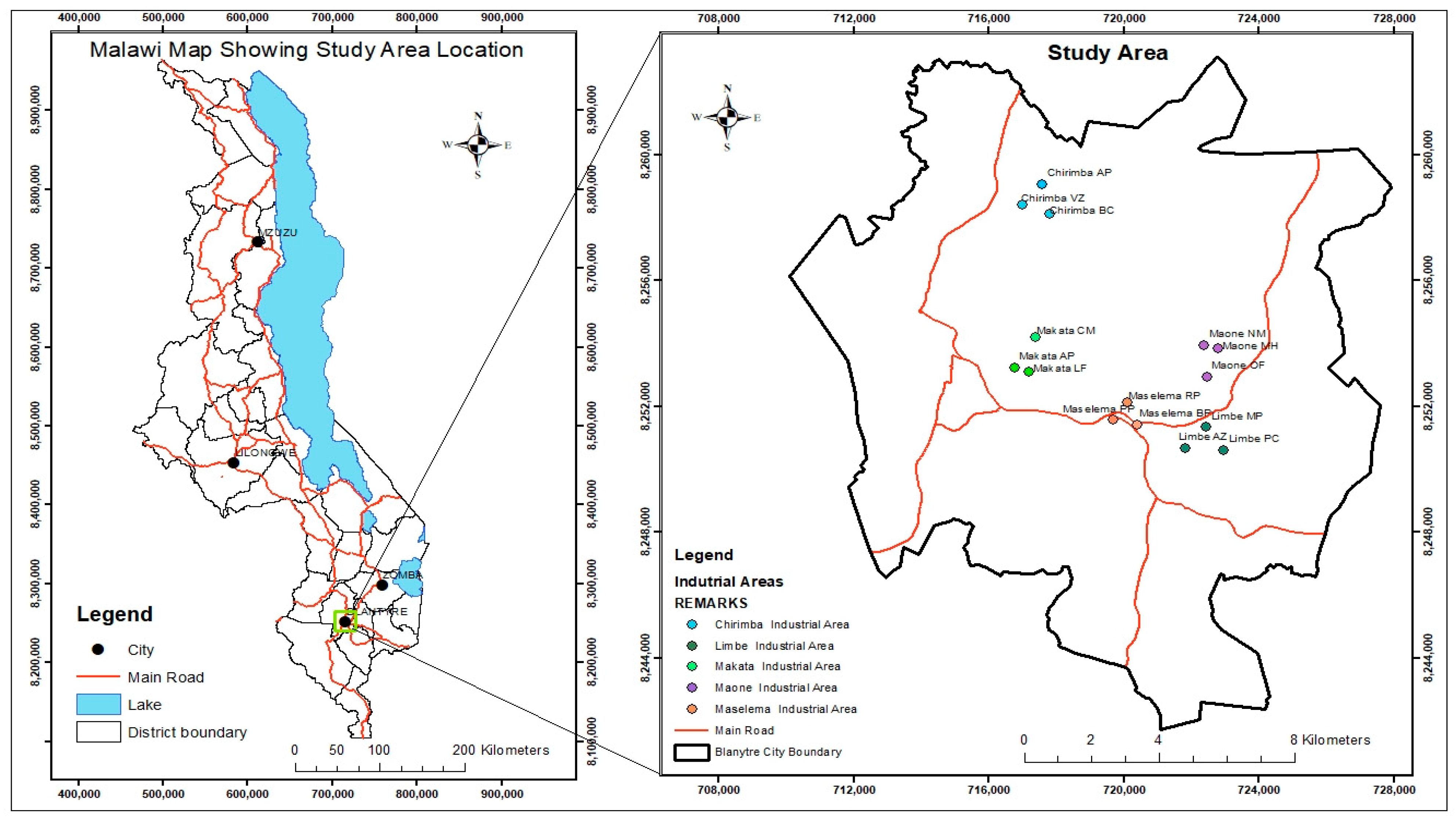
2.1. Description of Study Area

Blantyre City is the urban centre of Blantyre District in Malawi, which is found in the southern region of this nation at −15°29′59.99″ S, 35°00′0″ E and has an area of 240 km². Blantyre District has an overall population of about 1 million people [19].

The study was conducted at 15 sites selected from industrial zones, specifically Makata, Limbe, Maselema, Chirimba, and Maone, as shown in Figure 1, with corresponding Geographical Positioning System (GPS) coordinates provided in Appendix A.1. Monitoring of air quality concentrations and noise levels was performed in the rainy season (January–February 2023) and dry season (August–September 2023). All industrial zones are positioned alongside the main rivers or streams in Blantyre city, as they rely on water in their line production process, leading to the generation of effluents that are subsequently discharged into the water bodies [20]. Industries in Blantyre fall under the following categories: textile and leather products, paints, pharmaceuticals and other chemicals, metal and wood processing, petroleum and plastics, power distribution, dairy products and abattoir, beer breweries, tobacco processing, and food processing. The types of industries where monitoring happened in this work included plastic, food, metal processing, soap, cement, beverage, and furniture manufacturing industries.

2.2. Air Monitoring

Air quality monitoring was performed using an active mobile multi-gas monitor (Drager X-am 7000, manufactured by Dräger, Cheshire, UK) [21]. The monitor is equipped with electrochemical sensors that measured continuous concentrations of CO. A Dylos DC1100 PRO Laser Particle Counter (2018 model, manufactured by Dylos Coporation, Riverside, CA, USA) was used to monitor Particulate Matter (TSP, PM_2.5, and PM₁₀). Before sampling, the multi gas monitor was calibrated in air which was free of the gases measured according to the instrument operational manual provided by the manufacturer [21]. In all the locations, the equipment was placed at a minimum of 1.5 m from the ground to simulate the average breathing height. Air quality assessments at each site were in a set of 3, with each set consisting of 10 days, making a total number of sampled days being 30 per monitored site. The distance from the anticipated emission source was at least 30 m from the nearest building [22]. During data collection, 10 min consecutive average measurements were recorded in an Excel sheet during morning (09:00–10:30), midday (11:30–13:00), and afternoon (15:30–17:00), providing 10 sets of values per session per day which assisted in minimizing the volume of captured data. This was aimed at ensuring a wider range of data, which could lead to a better reliability of results [22]. These 3 distinct sampling sets were performed in the period of the rainy season in January–February 2023 and the dry season in August–September 2023.

2.3. Noise Monitoring

An Integrated Sound Level Meter (ISLM) was used for the assessment of noise levels. The selection of ISLM was made due to its appropriate statistic averaging technique, enabling the derivation of a succinct measure of the equivalent continuous sound pressure level (Leq). Prior to conducting measurements at each chosen site, the meter underwent calibration using the Castle Acoustic Calibrator, with the model specified as GA 601. The calibration was carried out according to the instrument operational manual provided by the manufacturer [23]. Noise measurement was conducted manually, with the instrument held at a height of 1.5 m above the ground and positioned 30 m away from the potential noise sources. The microphone was directed towards the primary noise source’s front, following the guidelines outlined by Castle Group Ltd. [23], to minimize the sound field. LAi (A-weighted instantaneous sound pressure level), which is an “A fast” scale, was used to record 30 measurements through 10 min consecutive average measurements during morning (09:00–10:30), midday (11:30–13:00), and afternoon (15:30–17:00), providing 10 sets of values per session per day [24]. These time intervals were selected to ensure that samples were collected during onset of production up to when the production was winding down. Noise level monitoring at each site was in a set of 3, with each set consisting of 10 days, making the total number of sampled days being 30 per monitored site. These 3 distinct sampling sets were performed in the period of the rainy season in January–February 2023 and the dry season in August–September 2023.

2.4. Data Analysis

The open-source software R Studio version 4.3.1 was used to analyse the data [25]. A t-test was used to observe the variations among the sample means and between the sample types, respectively, at 95% confidence interval. The Microsoft Excel 2007 Windows program was used to analyse data such as the geo-accumulation index. A significance level (α) of 0.05 was used for all statistical tests in this study. A Pearson (r) correlation examined the relationship between the levels of parameters in air with those of noise [26].

To quantitively identify the source of the AQPs in the study area, the Positive Matrix Factorization (PMF) model was used to analyse the data by using EPA PMF 5.0 (USA) software [27].

The HYSPLIT model by Air Resources Lab (National Oceanic and Atmospheric Administration, Silver Spring, MD, USA) was used to collect and determine the movement pattern of air pollutants through backward and forward trajectories as also used by Lv et al. [8].

PMF was calculated using Equation (1) below, where $X_{ij}$ is composed of the $j$-th compound concentration measured in the $i$-th sample, source contribution matrix $g_{ik}$ represents the contribution of the $k$-th source to the $i$-th sample, source profile matrix $f_{kj}$ is made up of the $j$-th compound from the $k$-th source, and $e_{ij}$ is the residual matrix.

$$X_{ij}={{\displaystyle \sum }}_{k=1}^p{g}_{ij}{f}_{kj}+e_{ij}$$

(1)

The objective of PMF analysis is to minimize Q as per Equation (2) below.

$$Q={{\displaystyle \sum }}_{i=1}^n{{\displaystyle \sum }}_{j=1}^m{\left[\frac{x_{ij}-{{\displaystyle \sum }}_{k=1}^p{g}_{ik}{f}_{kj}}{u_{ij}}\right]}^{2}subject to g_{ik}\ge 0 and f_{kj}\ge 0$$

(2)

PMF 5.0 requires the input of concentration of samples species as well as uncertainty. Equation (3) below is used to calculate uncertainty of the concentrations.

$$\sqrt{{\left(error fraction\times c\right)}^2+MD{L}^2}$$

For

$$c \le \mathit{MDL}, u_{ij} = 5/6 \times \mathit{MDL} \mathrm{For} c > \mathit{MDL}, u_{ij}$$

(3)

The factor numbers were configured to 2, 3, 4, 5, and 6, with 40 runs as a total to ensure stability of the model [28].

3. Results

3.1. Air Quality Parameters and Noise Levels

The values for air quality concentrations and noise levels in

Table 1. The mean values of air quality parameters (µg/m³) and noise levels (dB) during the dry and wet seasons.

Sampling Point	CO (mg/m3)		TSP (µg/m3)		PM10 (µg/m3)		PM2.5 (µg/m3)		Noise (dB)
	Wet Season	Dry Season	Wet Season	Dry Season	Wet Season	Dry Season	Wet Season	Dry Season	Wet Season	Dry Season
Maone MH	0 ± 0.00	0 ± 0.00	30.5 ± 13.37	112 ± 39.02	13.8 ± 2.70	21.3 ± 8.41	10.3 ± 2.61	16 ± 6.21	38.5 ± 5.90	49.1 ± 10.23
Maone NM	0.667 ± 0.58	1.7 ± 1.13	45.4 ± 19.97	95.9 ± 29.47	25.4 ± 11.25	27 ± 12.98	19 ± 8.35	20.3 ± 9.80	42.4 ± 8.26	47.5 ± 3.88
Maone OF	0 ± 0.00	0 ± 0.00	15 ± 6.10	75.7 ± 9.00	5.33 ± 1.89	13.6 ± 3.65	3.67 ± 1.36	10.3 ± 2.65	34.8 ± 1.30	45.6 ± 1.22
Limbe AZ	0 ± 0.00	0 ± 0.00	66.3 ± 52.10	105 ± 44.09	17 ± 15.97	24.7 ± 7.15	12.8 ± 11.87	18.7 ± 5.16	48.9 ± 2.24	47.8 ± 2.58
Limbe MP	0.333 ± 0.58	1.67 ± 0.58	214 ± 76.46	147 ± 37.82	36.2 ± 17.72	47.8 ± 16.68	27.1 ± 13.32	35.8 ± 12.58	51.9 ± 2.82	50.8 ± 5.99
Limbe PC	0 ± 0.00	0 ± 0.00	23.9 ± 14.11	115 ± 11.57	6.93 ± 3.52	26.6 ± 6.65	5.17 ± 2.63	20 ± 4.95	43.4 ± 6.02	48.9 ± 6.26
Maselema BP	2 ± 3.46	4.33 ± 2.31	174 ± 90.06	184 ± 114.00	18.3 ± 8.24	25.7 ± 7.91	13.8 ± 6.17	19.3 ± 5.91	58.4 ± 1.69	58.1 ± 2.69
Maselema PP	2.67 ± 3.06	3.67 ± 2.08	46.7 ± 25.67	184 ± 5.86	13.5 ± 7.82	25.7 ± 4.49	10.1 ± 5.84	19.3 ± 3.30	41.1 ± 1.10	47.4 ± 1.14
Maselema RP	1.33 ± 1.53	3 ± 2.00	44.9 ± 20.32	105 ± 27.59	4.3 ± 0.17	45.7 ± 13.36	12.5 ± 15.93	34.3 ± 10.00	39.4 ± 1.83	47.4 ± 3.32
Chirimba AP	0 ± 0.00	0.667 ± 1.15	319 ± 319.35	52.3 ± 5.61	23.1 ± 17.63	13.6 ± 5.98	17.1 ± 13.34	10.1 ± 4.61	53.5 ± 2.47	52.4 ± 5.09
Chirimba BC	0.33 ± 0.58	1.33 ± 0.58	18.3 ± 5.44	76.3 ± 37.86	5.07 ± 1.01	13.3 ± 6.91	3.6 ± 0.85	9.83 ± 5.27	39 ± 3.60	46.2 ± 0.67
Chirimba VZ	0 ± 0.00	0 ± 0.00	26.4 ± 6.92	68.7 ± 15.72	7.03 ± 2.03	15.7 ± 1.81	5.13 ± 1.46	11.8 ± 1.32	38.7 ± 3.95	46.7 ± 1.93
Makata AP	0 ± 0.00	1.33 ± 0.58	22 ± 6.75	51 ± 20.44	9.23 ± 2.35	21.6 ± 19.92	6.87 ± 1.76	16.4 ± 14.85	40.3 ± 2.27	51.6 ± 3.23
Makata CM	0 ± 0.00	0.667 ± 1.15	41 ± 3.79	50.4 ± 29.98	9.5 ± 2.51	17.1 ± 15.70	7.1 ± 1.91	12.7 ± 11.84	52.5 ± 4.82	47 ± 1.96
Makata LF	0 ± 0.00	1.33 ± 0.58	188 ± 272.32	75.6 ± 22.86	25.1 ± 27.10	25.9 ± 11.34	18.6 ± 20.50	19.4 ± 8.66	38.9 ± 5.53	42.5 ± 0.66
Malawi Standard	10 mg/m3		230 µg/m3		150 µg/m3		25 µg/m3		85 dB
WHO Standard	10 mg/m3		N/A		45 µg/m3		15 µg/m3		110 dB

Values are in the form of mean ± standard deviation.

are presented in comparison to the limits set by the World Health Organization and Malawi Standards for specific parameters [22,24,29,30].

3.1.1. Carbon Monoxide (CO) Concertation Levels

In the wet season, the range of CO concentration in the air was from 0 to 2.67 mg/m³, while in the dry season it was from 0 to 4.33 mg/m³ (Table 2). A comparison of the results showed that the dry season CO concertation levels were significantly higher (p < 0.05) than the wet season values. This might be attributed to washout of the pollutants by rainfall in the wet season. The air sampled from Maselema BP showed the highest concentrations of CO, measuring 2 mg/m³ during the wet season and 4.33 mg/m³ during the dry season. The concentration of CO was generally below the limit of Malawi [22] and WHO standards of 10 mg/m³ [29], as shown Figure 2. These elevated levels, potentially originating from vehicle emissions due to the nearby highway, align with the air mass trajectory at 500 m (shown in Figure 3). The figure indicates a predominant flow of air mass from the western side, contributing to the peak CO concertation levels at the site.

The trajectory in Figure 3 shows that the air was moving from the study area going towards the southeast. The concentrations recorded corresponded well with a study conducted by Mapoma et al. [15] on spatial variation of volatile organic compounds and carbon monoxide in Blantyre City, Malawi, which showed that the CO levels were found to be significantly higher (p < 0.05) than those found in a similar study of 2004. In research conducted by Ukpebor et al. [31] in Benin City, Nigeria, examining the effects of enhanced traffic control measures on air quality and noise levels in both commercial and unrestricted traffic areas, comparable findings were observed. The study revealed that CO levels ranged from 1.30 to 3.20 ppm after the implementation of traffic control measures. In the dry and wet season, 100% of CO values were within the Malawian and WHO Standards, respectively.

3.1.2. Total Suspended Particle Concertation Levels

In the wet season, maximum TSP concentration in the air was 319 µg/m³, while in the dry season it was 184 µg/m³ (Table 2). A comparison of rainy season and dry season air TSP values indicated no significant difference (p > 0.05). During the wet season, the highest TSP concentration was observed from air sampled at Chirimba AP, and was 319 µg/m³. During the dry season, the highest TSP concentration was observed from air sampled at Maselema BP and Maselema PP, both with values of 184 µg/m³. It was also observed that in some cases, the concentrations of TSP were higher in the wet season than during dry seasons. For example, during dry season monitoring, some sites such as Chirimba AP and Makata LF had lower concentrations of TSP in the higher season as compared to the dry season due to the fact that production was not at full capacity in these industries. This confirms that industries are contributing to pollution because once there is no production, the air quality seem to be better than when production is in full swing. The concentration of TSP was generally below the limit of Malawi Standard [22] of 230 µg/m³, as per Figure 4. These concentrations may have come from operations-related emissions, as more air mass at 500 m trajectory was moving from the sampling point to other surroundings within Malawi during the wet season, while in the dry season the levels could be emanating from surrounding areas, as per the trajectories shown in Figure 5. The concentrations recorded were much higher than 75 µg/m³, as recorded by Sarpong et al. [32], who studied PM_2.5, PM₁₀, and TSP exposure in the Tema Metropolitan area of Ghana, as well as by Sabuti and Mohamed [33], who found the level of TSP to be within the range of 13 to 74 µg/m³. In the wet season, 93% of TSP values were within the Malawi Standard, while 7% were above it, and in the dry season, 100% of the TSP values were within the allowable Malawi Standard.

3.1.3. PM₁₀ Concertation Levels

In the wet season, the range of PM₁₀ concentration in the air was from 4.3 to 36.2 µg/m³, while in the dry season it was from 13.3 to 47.8 µg/m³ (Table 2). The dry season PM₁₀ values were significantly higher (p < 0.05) than the wet season values. The concentration of PM₁₀ was generally below the limit of the Malawian [22] and WHO [29] standards of 150 and 45 µg/m³, as per Figure 6. The highest PM₁₀ concentrations were observed from air sampled from Limbe MP, and were 36.2 µg/m³ as well as 47.8 µg/m³ during the wet season and dry seasons, respectively (which may have come from operations-related emissions, as more air mass at 500 m trajectory was moving from the sampling point to other surroundings within Malawi in the wet season, while in the dry season, the levels could be emanating from surrounding industries in Malawi, as per trajectories in Figure 7). The concentrations recorded were lower than 56.24 µg/m³, recorded by Sarpong et al. [32], who studied PM_2.5, PM₁₀, and total suspended particle exposure in the Tema Metropolitan Area of Ghana, but were higher than the 20.7 µg/m³ concentration recorded in 2017 found by Rovira et al. [34] in a study conducted in Catalonia, Spain, on air quality, health impacts, and burden of disease due to air pollution (PM₁₀, PM_2.5, NO₂, and O₃). In the wet season, 100% of TSP values were within the Malawian and WHO Standards, respectively. In the dry season, 100% of the values were within Malawi Standard and 87% were within the WHO standard, while the remainder (13%) were above this international standard.

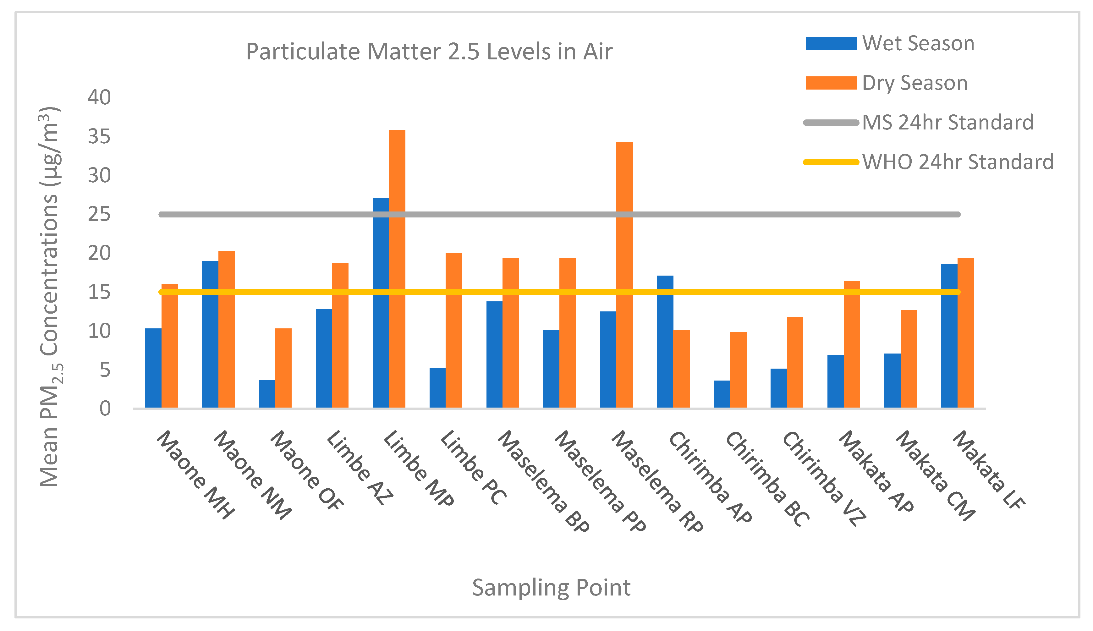
3.1.4. Particulate Matter 2.5 Concentration Levels

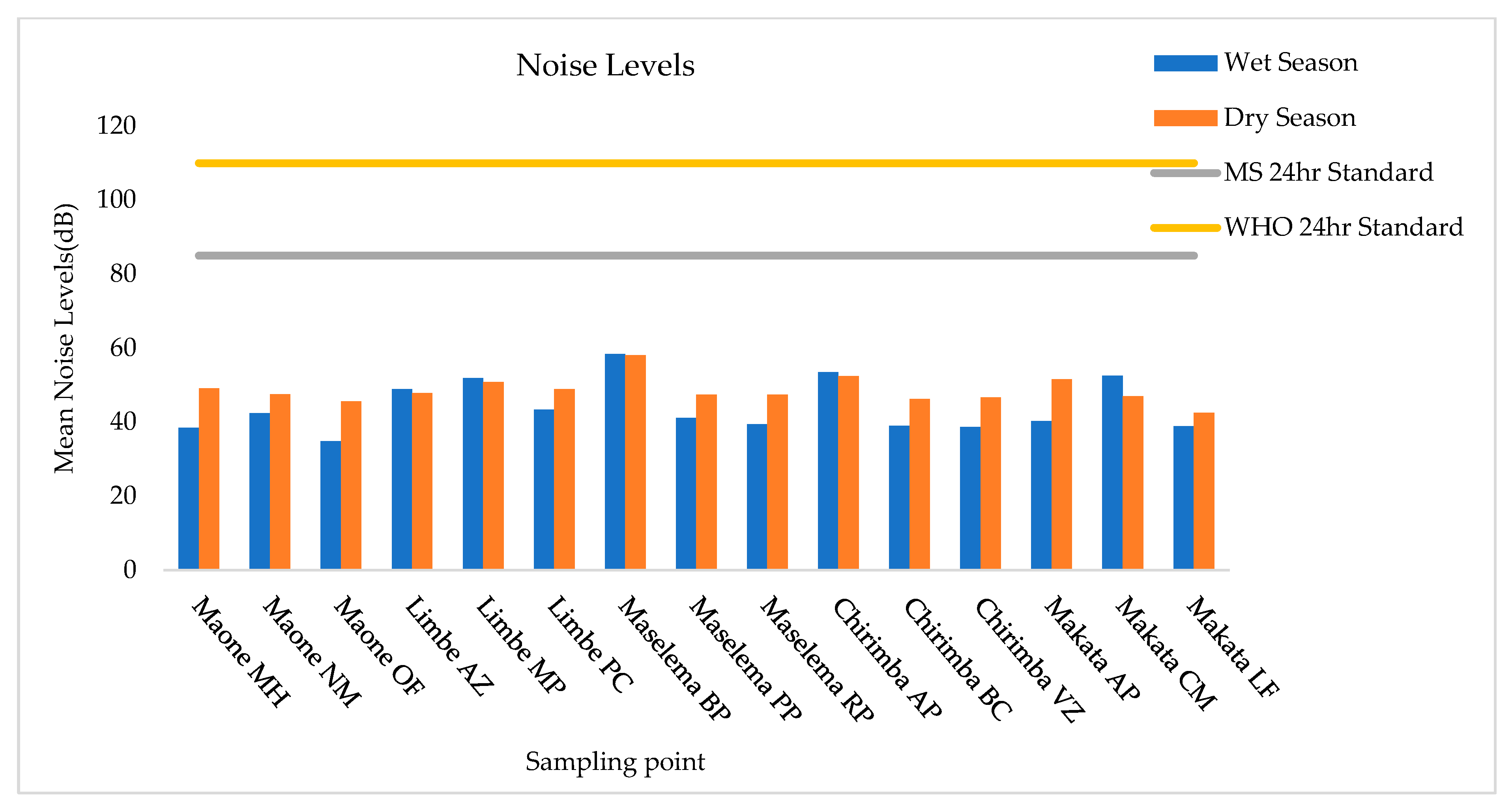
In the wet season, the range of PM_2.5 concentration in the air was from 3.6 to 27.1 µg/m³, while in the dry season it was from 9.83 to 35.8 µg/m³ (Table 2). The dry season PM_2.5 values were significantly higher (p < 0.05) than the dry season values. The concentration of PM_2.5 was generally below the limit of the Malawian [22] and WHO [29] standards of 25 and 15 µg/m³, as per Figure 8. The highest PM_2.5 concentrations were observed from air sampled from Limbe MP, and were 27.1 µg/m³ as well as 35.8 µg/m³ during the wet season and dry seasons, respectively (which may have come from operations-related emissions, as more air mass at 500 m trajectory was moving from the sampling point to other surroundings in the wet season, while in the dry season the levels could be emanating from surrounding industries, as per the trajectories in Figure 9). The concentrations recorded were lower than 38.09 µg/m³, recorded by Sarpong et al. [32], who studied PM_2.5, PM₁₀, and total suspended particle exposure in the Tema Metropolitan Area of Ghana, but were higher than the 11.8 µg/m³ concentration recorded in 2017 found by Rovira et al. [34], in a study conducted in Catalonia, Spain, on air quality, health impacts, and burden of disease due to air pollution (PM₁₀, PM_2.5, NO₂, and O₃). In the wet season, 93% of PM_2.5 values were within the Malawian standard while 7% were above this standard, and 73% of the values were within the WHO Standard while 27% of these were above it. In the dry season, 93% of the values were within Malawi Standard while 7% were above this standard, and 40% were within the WHO standard while the remainder of 60% of were above it.

3.1.5. Noise Levels

In the wet season, the range of Noise level was from 34.8 to 58.4 dB, while in the dry season it was from 42.5 to 58.1 dB (Table 2). Comparison of wet season and dry season Noise level values indicated a significant difference (p = 0.0011). The highest Noise level readings were observed from Maselema BP, and were 58.4 dB as well as 58.1 dB during the wet season and dry seasons, respectively (which may have come from vehicle movement and honking, as the highway is in proximity). Higher Noise level readings were recorded from Chirimba AP and Limbe MP. Chirimba AP noise level readings were 53.5 dB as well as 52.4 dB during the wet season and dry seasons, respectively. Limbe MP noise level readings were 51.9 dB as well as 50.8 dB during the wet season and dry seasons, respectively. The concentrations recorded by Manojkumar et al. [5], who conducted the assessment, prediction, and mapping of noise levels in Vellore City, India, were much higher and were within the range of 67–87 dB. A study on the impacts of improved traffic control measures on air quality and noise level in Benin City, Nigeria, by Ukpebor et al. [31] found different results of noise levels which were much higher, in the range of 70 to 79 dB, after traffic control measures were put in place. The Noise level was generally below the limit of the Malawian [24] and WHO [30] standards of 85 and 110 dB, respectively, as per Figure 10. In the wet and dry seasons, 100% of the Noise level values were within the Malawian and WHO Standards.

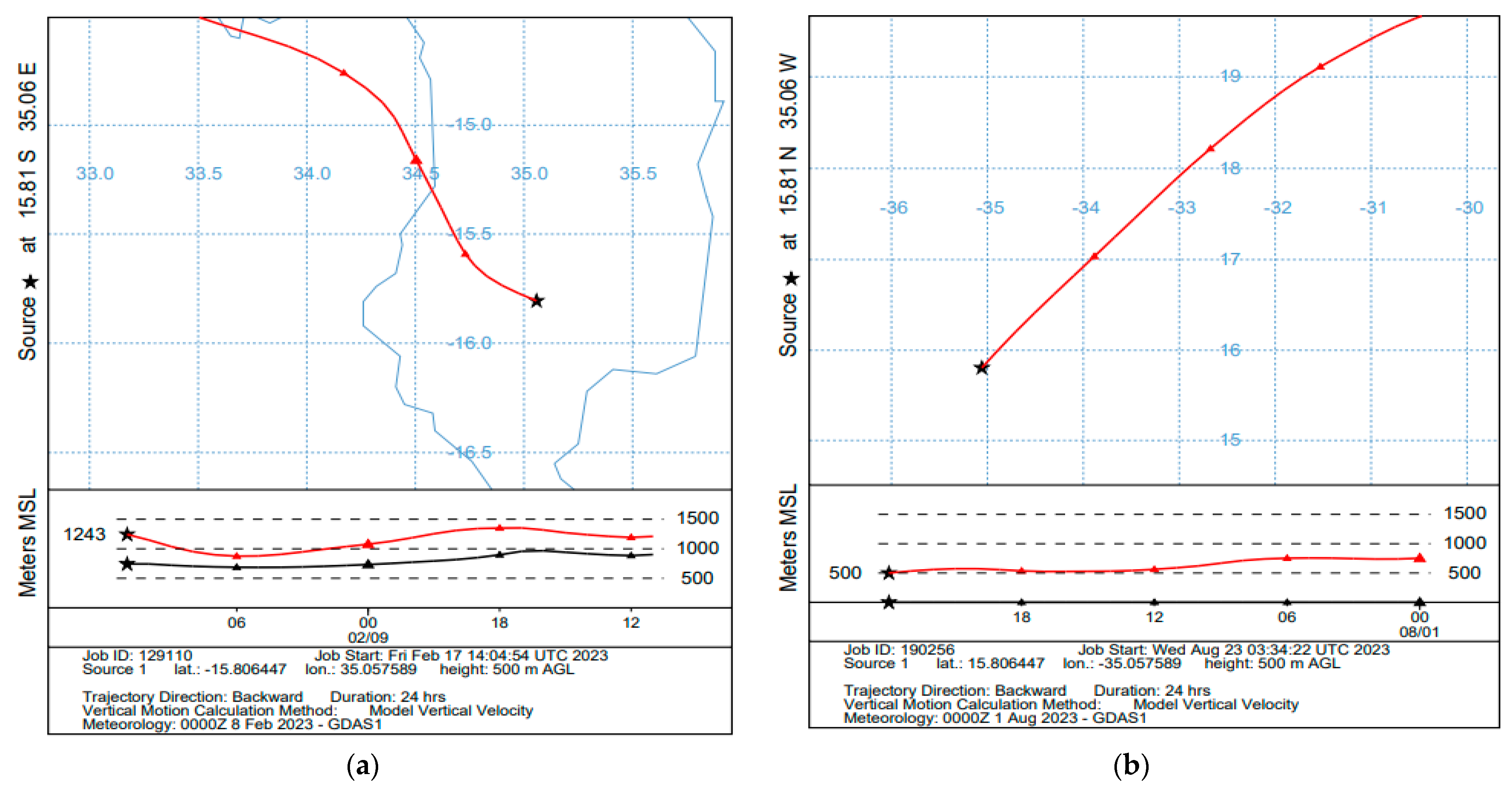
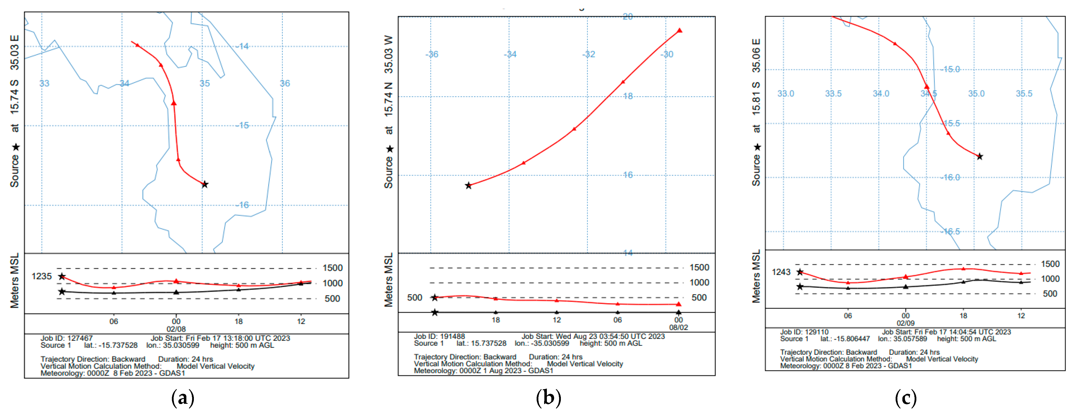
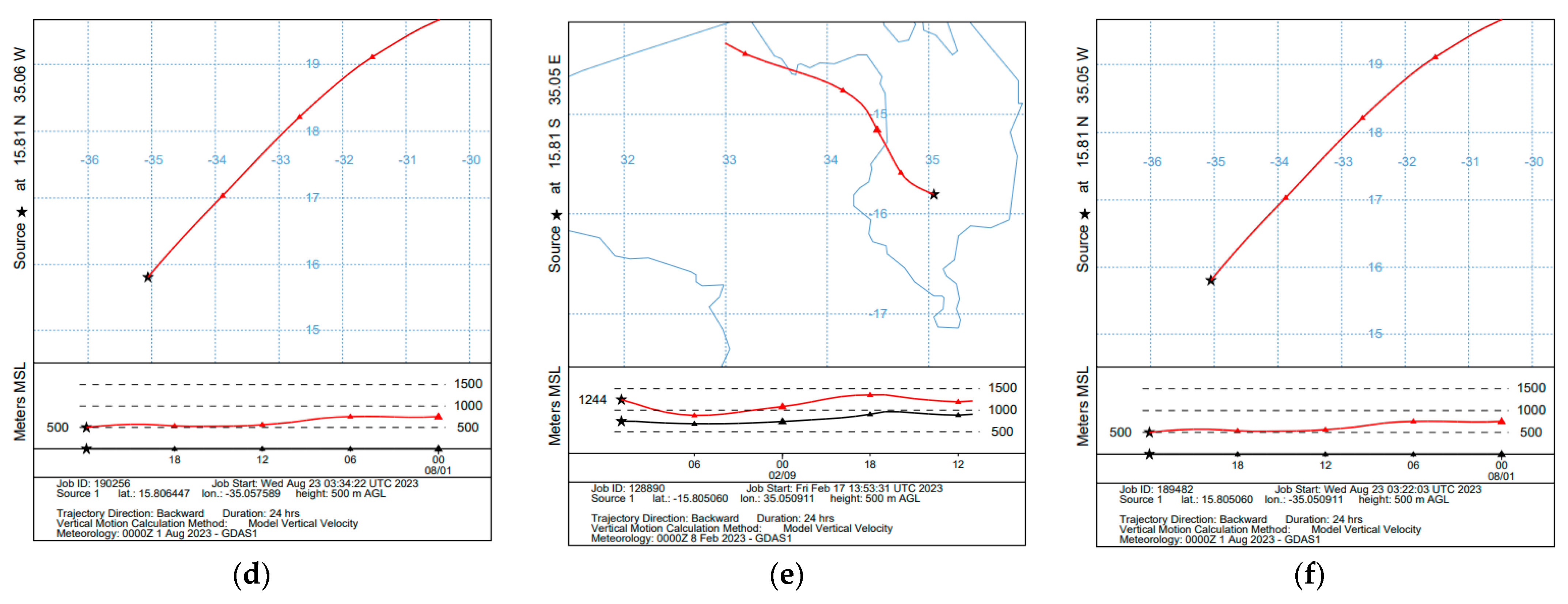
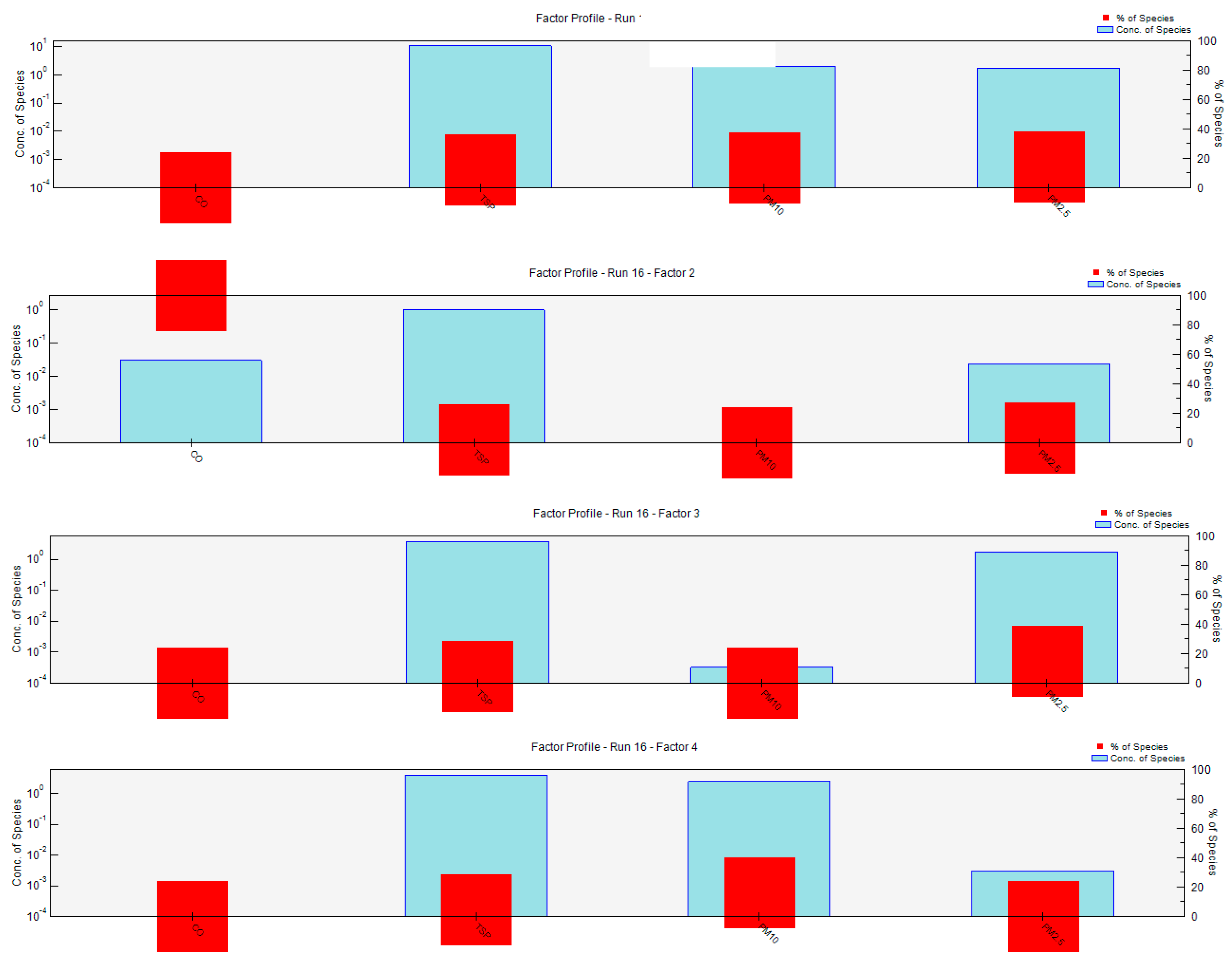
3.2. Source Apportionment (Examination of Sources) for Air Quality Parameters from the Industrial Areas

After using the PMF model with a factor count of six, the difference between Qtrue and Qrobust were minimum and stable. The scaled residuals for air quality parameters exhibited values ranging from 0.00746 to 0.00773 during the dry season, while registering at 0.00002 during the wet season. This suggests that the parameters follow a normal distribution, as the values fall within the range of +3 to −3 [27]. Furthermore, this means that the model is reliable and the Factor Analysis in the Section above is accurate. In the dry season, the signal-to-noise (S/N) ratios for all air quality parameters varied between 0.609 and 3.693, while during the wet season, the range was 0.091 to 2.314 (Table 2). This variability indicates that CO, TSP, PM₁₀, and PM_2.5 exhibited signals ranging from “poor” to “strong,” with TSP registering the highest concentration. This underscores the importance for industries engaged in metal processing and beverage manufacturing to enhance their emission management practices throughout both the dry and wet seasons.

Table 2. The signal-to-noise ratio of air quality parameters during the dry and wet seasons.

	S/N Values
Species	Dry Season	Wet Season
CO	0.609	0.091
TSP	3.693	1.843
PM10	2.426	2.314
PM2.5	2.466	1.528

Table 2. The signal-to-noise ratio of air quality parameters during the dry and wet seasons.

	S/N Values
Species	Dry Season	Wet Season
CO	0.609	0.091
TSP	3.693	1.843
PM10	2.426	2.314
PM2.5	2.466	1.528

As per Figure 11, Figure 12, Figure 13 and Figure 14 below, during dry season in Factor 1, TSP, and CO provided 25.1% and 0.6% respective contributions. The contribution of the various parameters to each factor was shown in the factor fingerprints (Figure 12 and Figure 14). During the wet season in Factor 1, PM_2.5, PM₁₀, and TSP provided 14.8%, 14.1%, and 12.7% of the respective contributions. As demand for cement is high for development purposes, TSP levels are usually high around cement production plants [35]. Furthermore, the outcome of a study conducted by Olatunde et al. [36] present important data on pollution of soils by heavy metals around Dangote cement factory, Ibese, which showed the need for an overhaul of the waste management initiatives of the factory and an emphasis on complying with the regulatory from relevant agencies. Another study by Egbe et al. [37] highlighted that that cement production processes are a source of pollutants through deposition. This makes Factor 1 linked to cement manufacturing industries.

During dry season in Factor 2, CO, PM_2.5, and PM₁₀ provided 55.1%, 13.6%, and 13.5% respective contributions. During the wet season in Factor 2, CO, PM_2.5, and TSP provided 100%, 3.5%, and 2.1% respective contributions. As shown in a previous study by Mapoma et al. [15], the increased levels of CO may be due to emissions coming from the moving vehicles along the roads. Another study conducted by Zhu et al. [38] stated that industrial, facilities such as factories, emit a variety of pollutants such as CO. Studies conducted by many authors showed that one of the well-known types of air pollutants found in urban areas is CO, which is mostly sourced from fossil fuel use such as coal and gasoline [39,40,41,42], which the sampling sites utilize during production processes. As such, whilst considering the parameter concentration distribution as well as aspects in Section 3.1.1 to 3.1.4, Factor 2 represents the food production industries.

During the dry season in Factor 3, PM_2.5 and PM₁₀ provided 11.1% and 10.9% of the respective contributions. During the wet season in Factor 3, PM_2.5 and TSP provided 15.2% and 4.5% of the respective contributions. A study conducted by Yuan et al. [43] showed that the putty and sanding processes in furniture making increases levels of particulate matter less than 2 µm. Another study by Zheng and Xu [44] showcased the role which furniture manufacturing companies take in PM 2.5 emission and how the impact needs to be mitigated. A study by Ro’in et al. [45] also illustrated that wood sanding production in the furniture production process exhibits the highest level of dust which means that Factor 3 includes furniture manufacturing industries.

During dry season in Factor 4, PM₁₀, PM_2.5, TSP and CO provided 57.8%, 57.6%, 46.2%, and 2.0% respective contributions. During the wet season in Factor 4, PM₁₀, and TSP provided 16.7% and 4.6% of the respective contributions. A study by Yusuf et al. [46] highlighted that the levels of PM₁₀ increased significantly in a plastic-processing industry which corresponds with the percentage of carbon monoxide seen here. Aspects in Section 3.1.1 to Section 3.1.4 should also be put into consideration. Another study by Alves et al. [47] showed that the plastics industry was a source of PM 10 in road dust. A study by Chirino et al. [48] also states that plastic manufacturing industries are one of the main sources of PM₁₀ emission into the environment. Therefore, Factor 4 represents the plastic manufacturing industries.

During dry season in Factor 5, TSP and CO provided 26.7% and 24.7% respective contributions. During wet season in Factor 5, PM₁₀, PM_2.5, and TSP provided 41.9%, 41.9%, and 1.5% contributions. Ashrafi et al. [49] stated that metal production is one of the industrial processes causing the higher value of TSP. Another study conducted by Sonibare and Akeredolu [50] stated that a common source of TSP is the metal processing industry as the grinding and heating processes among others are employed. A study by Guol et al. [51] iterated that the steel and iron producing industries were common sources of TSP. This means that Factor 5 represents metal processing and manufacturing industries.

During dry season in Factor 6, CO, PM_2.5, PM₁₀, and TSP provided 18.2%, 17.7%, 17.6%, and 2% of the respective contributions. During the wet season in Factor 6, TSP, PM₁₀, and PM_2.5 provided 74.4%, 27%, and 24.6% of the respective contributions. One of the main sources of TSP and CO is the food and beverage industry through the heating, fuel utilization, as well as machinery processing aspects [52]. Furthermore, a study conducted by Jadoon and Nawazish [53], stated that some of the common sources of CO are industrial boilers and incomplete combustion processes from food and beverage manufacturing industries. As such, it reflects the percentages seen here, and may mean that Factor 6 represents the beverage manufacturing industries.

As such, this means that during both wet seasons the plastic manufacturing industries contribute highly towards TSP in the air around the industrial sites which means that mitigation measures need to be implemented accordingly. This should be extended to food manufacturing industries which are the highest contributing sources of CO in the air during the dry and wet season. The other industries, namely metal processing and beverage manufacturing are also sources of PM_2.5, PM₁₀, and CO and need to be targeted for needed remedial actions.

3.3. Correlation between Air Quality Parameters and Noise Levels

Correlations were conducted between air quality parameters and noise levels for both seasons. This was performed to determine whether air quality parameters can be used as an indicator for noise level pollution. The following were the correlations as per

Table 3. Correlations between air quality parameters and noise level.

Variable	Noise Level
	Dry Season	Wet Season
CO	0.205 (0.177)	0.062 (0.687)
TSP	0.241 (0.110)	0.401 (0.006)
PM10	0.011 (0.941)	0.358 (0.016)
PM2.5	0.011 (0.942)	0.306 (0.041)

Brackets have the significance levels.

below, which shows that air quality has an influence on noise levels. CO correlation with noise is shown to be lower during the wet season as compared to the dry season. It is also observed that air quality has an influence on noise levels with a seasonality effect, as we can see the correlations between (TSP, PM₁₀, and PM_2.5) and noise level changes from weak during dry season to moderately strong in the wet season. The positive correlation between air quality parameters and noise levels suggests potential shared sources or synergistic effects, and as such, further investigations are needed to understand the mechanisms driving these associations. This kind of correlation is also seen in various studies, such as the one conducted by Lacerda et al. [54], who compared the hearing thresholds of two groups of workers—one exposed to both noise (90 dB) and CO and another exposed solely to noise (90 dB). The findings indicated a significant increase in hearing thresholds (at high frequencies of 3, 4, and 6 kHz) in the “noise  +  CO group” when compared to the “noise group”.

4. Conclusions

This study determined the concentration levels of air quality (CO, TSP, PM_2.5, and PM₁₀) and noise from industrial sites (Makata, Limbe, Maselema, Chirimba, and Maone). During the wet season, CO, TSP, PM₁₀, and PM_2.5 averaged 0.49 ± 0.65 mg/m³, 85.03 ± 62.18 µg/m³, 14.65 ± 8.13 µg/m³, and 11.52 ± 7.19 µg/m³, respectively, whereas in the dry season, the average concentrations rose to 1.31 ± 0.81 mg/m³, 99.86 ± 30.06 µg/m³, 24.35 ± 9.53 µg/m³, and 18.28 ± 7.14 µg/m³. In the wet season, the highest concentrations of CO, TSP, PM₁₀, and PM_2.5 were 2.67 ± 3.06 mg/m³, 319 ± 319.35 µg/m³, 36.2 ± 17.72 µg/m³, and 27.1 ± 13.32 µg/m³, respectively. Dry season highest concentrations were 4.33 ± 2.31 mg/m³, 184 ± 114.00 µg/m³, 47.8 ± 16.68 µg/m³, and 35.8 ± 12.58 µg/m³. Noise levels remained below MS and WHO standards. The study also determination of movement pattern of the air pollutants using trajectory models from the National Oceanic and Atmospheric Administration (NOAA). The study found that the concentrations of air quality parameters generally remained within the permissible limits set by Malawi and the World Health Organization (WHO), except for a limited number of samples. This deviation was attributed to the movement of air masses, as indicated by the generated trajectories. Noise levels were found to be within the maximum allowable standard of Malawi and the WHO. Correlations between air quality parameters and noise levels were made which showed a seasonality effect, as such air quality has an influence on noise pollution.

The analysis results of the Positive Matrix Factorization (PMF) model indicated that there were six main factors affecting the accumulation of air quality parameters, namely: (1) plastic manufacturing industries, (2) food manufacturing industries, (3) metal processing and manufacturing industries, (4) cement manufacturing industries, (5) beverage manufacturing industries, and (6) furniture manufacturing industries.

Recommendations

Future PMF assessments need to be performed to include other parameters such as Nitrogen dioxide (NO₂), Sulfur dioxide (SO₂), and Volatile Organic Carbons (VOCs), which are also important since they may be of concern to the health of people, but were not included due to time and financial limitations. Further studies should be conducted to better understand the factors affecting the PMF flow dynamics in the industrial zones and their influence. These should include climatological factors (wind, precipitation, and temperature). There is a need to collect samples during the nighttime, which was not performed due to security concerns, since the sampling was not conducted within the industrial compounds.

References

1. Russell, V.S. Pollution: Concept and definition. In Biological Conservation, 3rd ed.; Australian National University: Canbera, Australia, 1974; Volume 6, pp. 157–161. [Google Scholar] [CrossRef]
2. Thulu, F.G.D.; Tembo, D.; Nyirongo, R.; Mzaza, P.J.C.; Kamfosi, A.; Mawenda, U.C. Electromagnetic Frequency Pollution in Malawi: A Case of Electric Field and Magnetic Flux Density Pollution in Southern Africa. Int. J. Environ. Res. Public Health 2023, 20, 4413. [Google Scholar] [CrossRef] [PubMed]
3. Assanov, D.; Zapasnyi, V.; Kerimray, A. Air quality and industrial emissions in the cities of Kazakhstan. Atmosphere 2021, 12, 314. [Google Scholar] [CrossRef]
4. Hsu, C.Y.; Chi, K.H.; Wu, C.D.; Lin, S.L.; Hsu, W.C.; Tseng, C.C.; Chen, M.J.; Chen, Y.C. Integrated analysis of source-specific risks for PM2.5-bound metals in urban, suburban, rural, and industrial areas. Environ. Pollut. 2021, 275, 116652. [Google Scholar] [CrossRef] [PubMed]
5. Manojkumar, N.; Basha, K.; Srimuruganandam, B. Assessment, Prediction and Mapping of Noise Levels in Vellore City, India. Noise Mapp. 2019, 6, 38–51. [Google Scholar] [CrossRef]
6. Bai, L.; Wang, J.; Ma, X.; Lu, H. Air pollution forecasts: An overview. Int. J. Environ. Res. Public Health 2018, 4, 780. [Google Scholar] [CrossRef] [PubMed]
7. World Bank. Malawi Country Environmental Analysis. Malawi Country Environmental Analysis; World Bank: Pretoria, South Africa, 2019. [Google Scholar] [CrossRef]
8. Lv, B.; Liu, Y.; Yu, P.; Zhang, B.; Bai, Y. Characterizations of PM2.5 pollution pathways and sources analysis in four large cities in China. Aerosol Air Qual. Res. 2015, 5, 1836–1843. [Google Scholar] [CrossRef]
9. Maqsood, N.; Younes, I.; Minallah, M.N. Industrial Noise Pollution and Its Impact on the Hearing Capacity of Workers: A Case Study of Gujranwala City, Pakistan. Int. J. Econ. Environ. Geol. 2019, 2, 45–49. [Google Scholar] [CrossRef]
10. Osei, F.A.; Effah, E.A. Health Effects caused by Noise—The Case of Africa: Evidence in Literature from the Past 25 Years. Asian J. Adv. Res. Rep. 2022, 16, 19–27. [Google Scholar] [CrossRef]
11. Chirwa, I.; Mlatho, J.S.; Kamunda, C.; Mikeka, C. Assessment of noise levels in heavy and light industries in Blantyre City, Malawi. Malawi J. Sci. Technol. 2019, 1, 73–92. [Google Scholar]
12. Sun, Y.; Tian, Y.; Xue, Q.; Jia, B.; Wei, Y.; Song, D.; Huang, F.; Feng, Y. Source-specific risks of synchronous heavy metals and PAHs in inhalable particles at different pollution levels: Variations and health risks during heavy pollution. Environ. Int. 2021, 146, 106162. [Google Scholar] [CrossRef]
13. Nazzal, Y.; Orm, N.B.; Barbulescu, A.; Howari, F.; Sharma, M.; Badawi, A.E.; Al-Taani, A.A.; Iqbal, J.; Ktaibi, F.E.; Xavier, C.M.; et al. Study of atmospheric pollution and health risk assessment: A case study for the sharjah and ajman emirates (uae). Atmosphere 2021, 11, 1442. [Google Scholar] [CrossRef]
14. Wang, Y.; Guo, G.; Zhang, D.; Lei, M. An integrated method for source apportionment of heavy metal(loid)s in agricultural soils and model uncertainty analysis. Environ. Pollut. 2021, 276, 116666. [Google Scholar] [CrossRef] [PubMed]
15. Mapoma, H.W.T.; Xie, X. State of Air Quality in Malawi. J. Environ. Prot. 2013, 4, 1258–1264. [Google Scholar] [CrossRef]
16. Tilley, E.; Chilunga, H.; Kwangulero, J.; Schöbitz, L.; Vijay, S.; Heilgendorff, H.; Kalina, M. “It is unbearable to breathe here”: Air quality, open incineration, and misinformation in Blantyre, Malawi. Front. Public Health 2023, 11, 1242726. [Google Scholar] [CrossRef]
17. Saleh, S.; Sambakunsi, H.; Mortimer, K.; Morton, B.; Kumwenda, M.; Rylance, J.; Chinouya, M. Exploring smoke: An ethnographic study of air pollution in rural Malawi. BMJ Glob. Health 2021, 6, e004970. [Google Scholar] [CrossRef] [PubMed]
18. Commonwealth Network. Available online: https://www.commonwealthofnations.org/about-us-commonwealth-network/ (accessed on 14 January 2024).
19. National Statistical Office. Malawi Population and Housing Census Main Report. Malawi Population and Housing Census Report. Government of Malawi, Zomba, 2019; Issue May, pp. 138–172. Available online: https://malawi.unfpa.org/sites/default/files/resource-pdf/2018%20Malawi%20Population%20and%20Housing%20Census%20Main%20Report%20%281%29.pdf (accessed on 28 December 2023).
20. BCA (Blantyre City Assembly). A Profile of Industries under Pollution Monitoring Programme of Blantyre City Assembly; BCA: Blantyre, Malawi, 2006. [Google Scholar]
21. Drager. Available online: www.draeger.co.uk (accessed on 14 January 2024).
22. MSB. Industrial Emissions-Emission from Mobile Sources and Stationary Sources_ Specification, 3rd ed.; Malawi Standards Board: Blantyre, Malawi, 2021. [Google Scholar]
23. CastleGroupLtd. Operating Manual: Pocket Sound level Meter Range (GA213, GA215 and GA256); CastleGroupLtd.: Scarborough, England, 2014. [Google Scholar]
24. Malawi Standards- MS 697:2021; Industrial Noise Affecting Mixed Residential and Industrial Areas for Rating, 3rd ed. Malawi Standards Board: Blantyre, Malawi, 2021.
25. Integrated Development for R. RStudio, Inc. Available online: http://www.rstudio.com (accessed on 14 January 2024).
26. Campos, P.M.D.; Esteves, A.F.; Leitão, A.A.; Pires, J.C.M. Design of air quality monitoring network of Luanda, Angola: Urban air pollution assessment. Atmos. Pollut. Res. 2021, 8, 101128. [Google Scholar] [CrossRef]
27. USEPA. EPA Positive Matrix Factorization (PMF) 5.0 Fundamentals and User Guide; U.S. Environment Protection Agency: Washington, DC, USA, 2014.
28. Guan, Q.; Wang, L.; Wang, F.; Pan, B.; Song, N.; Li, F.; Lu, M. Phosphorus in the catchment of high sediment load river: A case of the Yellow River, China. Sci. Total Environ. 2016, 572, 660–670. [Google Scholar] [CrossRef] [PubMed]
29. World Health Organization. WHO Global Air Quality Guidelines. Particulate Matter (PM2.5 and PM10), Ozone, Nitrogen Dioxide, Sulfur Dioxide and Carbon Monoxide; WHO: Geneva, Switzerland, 2021.
30. Berglund, B.; Lindvall, T.; Schwela, D.H. New Who Guidelines for Community Noise. Noise Vib. Worldw. 2000, 4, 24–29. [Google Scholar] [CrossRef]
31. Ukpebor, J.E.; Omagamre, E.W.; Bamidele, A.; Unuigbe, C.A.; Dibie, E.N.; Ukpebor, E.E. Impacts of improved traffic control measures on air quality and noise level in Benin City, Nigeria. Malawi J. Sci. Technol. 2021, 2, 51–83. Available online: https://www.ajol.info/index.php/mjst/article/view/218545 (accessed on 17 April 2024).
32. Sarpong, S.A.; Donkoh, R.F.; Konnuba, J.K.; Ohene-agyei, C.; Lee, Y. Analysis of PM2.5, PM10, and Total Suspended Particle Exposure in the Tema Metropolitan Area of Ghana. Atmosphere 2021, 12, 700. [Google Scholar] [CrossRef]
33. Sabuti, A.A.; Mohamed, C.A.R. Correlation between total suspended particles and natural radionuclide in malaysia maritime air during haze event in june-july 2009. J. CleanWAS 2018, 1, 1–5. [Google Scholar] [CrossRef]
34. Rovira, J.; Domingo, J.L.; Schuhmacher, M. Air quality, health impacts and burden of disease due to air pollution (PM10, PM2.5, NO2 and O3): Application of AirQ+ model to the Camp de Tarragona County (Catalonia, Spain). Sci. Total Environ. 2020, 703, 135538. [Google Scholar] [CrossRef]
35. Jayadipraja, E.; Daud, A.; Assegaf, A.; Maming, M. The application of the AERMOD model in the environmental health to identify the dispersion area of total suspended particulate from cement industry stacks. Int. J. Res. Med. Sci. 2016, 4, 2044–2049. [Google Scholar] [CrossRef]
36. Olatunde, K.A.; Sosanya, P.A.; Bada, B.S.; Ojekunle, Z.O.; Abdussalaam, S.A. Distribution and ecological risk assessment of heavy metals in soils around a major cement factory, Ibese, Nigeria. Sci. Afr. 2020, 9, e00496. [Google Scholar] [CrossRef]
37. Egbe, E.R.; Chinyere Nsonwu-Anyanwu, A.; Offor, S.J.; Opara Usoro, C.A.; Etukudo, M.H. Heavy metal content of the soil in the vicinity of the united cement factory in Southern Nigeria. J. Adv. Environ. Health Res. 2019, 7, 122–130. [Google Scholar] [CrossRef]
38. Zhu, T.; Tang, M.; Gao, M.; Bi, X.; Cao, J.; Che, H.; Chen, J.; Ding, A.; Fu, P.; Gao, J.; et al. Recent Progress in Atmospheric Chemistry Research in China: Establishing a Theoretical Framework for the “Air Pollution Complex”. Adv. Atmos. Sci. 2023, 40, 1339–1361. [Google Scholar] [CrossRef]
39. Anderson, B.; Bartlett, K.; Frolking, S.; Hayhoe, K.; Jenkins, J.; Salas, W. Methane and Nitrous Oxide Emissions from Natural Sources. 194. 2010. Available online: https://nepis.epa.gov/Exe/ZyNET.exe/P100717T.txt?ZyActionD=ZyDocument&Client=EPA&Index=2006%20Thru%202010&Docs=&Query=&Time=&EndTime=&SearchMethod=1&TocRestrict=n&Toc=&TocEntry=&QField=&QFieldYear=&QFieldMonth=&QFieldDay=&UseQField=&IntQFieldOp=0&ExtQFieldOp=0&XmlQuery=&File=D%3A%5CZYFILES%5CINDEX%20DATA%5C06THRU10%5CTXT%5C00000017%5CP100717T.txt&User=ANONYMOUS&Password=anonymous&SortMethod=h%7C-&MaximumDocuments=1&FuzzyDegree=0&ImageQuality=r75g8/r75g8/x150y150g16/i425&Display=hpfr&DefSeekPage=x&SearchBack=ZyActionL&Back=ZyActionS&BackDesc=Results%20page&MaximumPages=1&ZyEntry=22&slide (accessed on 12 November 2023).
40. Chen, R.; Pan, G.; Zhang, Y.; Xu, Q.; Zeng, G.; Xu, X.; Chen, B.; Kan, H. Ambient carbon monoxide and daily mortality in three Chinese cities: The China Air Pollution and Health Effects Study (CAPES). Sci. Total Environ. 2011, 23, 4923–4928. [Google Scholar] [CrossRef] [PubMed]
41. Ho, K.F.; Lee, S.C.; Chan, C.K.; Yu, J.C.; Chow, J.C.; Yao, X.H. Characterization of chemical species in PM2.5 and PM10 aerosols in Hong Kong. Atmos. Environ. 2003, 37, 31–39. [Google Scholar] [CrossRef]
42. Sun, S.; Li, L.; Wu, Z.; Gautam, A.; Li, J.; Zhao, W. Variation of industrial air pollution emissions based on VIIRS thermal anomaly data. Atmos. Res. 2020, 244, 105021. [Google Scholar] [CrossRef]
43. Yuan, N.; Zhang, J.; Lu, J.; Liu, H.; Sun, P. Analysis of inhalable dust produced in manufacturing of wooden furniture. BioResources 2014, 4, 7257–7266. [Google Scholar] [CrossRef]
44. Zheng, H.; Xu, L. Production, and consumption—based primary PM2.5 emissions: Empirical analysis from China’s interprovincial trade. Resour. Conserv. Recycl. 2020, 155, 104661. [Google Scholar] [CrossRef]
45. Ro’in, F.; Raharjo, M.; Setiani, O. Association Between PM2.5 Wood Dust Exposure and Acute Respiratory Infection on Plywood Industry Workers in PT. Muara Kayu Sengon, Jatilawang District, Banyumas Regency. In Proceedings of the E3S Web of Conferences, Semarang, Indonesia, 8–9 August 2023; EDP Sciences: Les Ulis, France, 2023; Volume 448, p. 05009. [Google Scholar]
46. Yusuf, S.Y.; Rahim, N.A.A.A.; Wazam, W.Z.; Naidu, D.; Jamian, R. Indoor and outdoor particulate matter concentrations in the vicinity of plastic waste processing industries. IOP Conf. Ser. Earth Environ. Sci. 2020, 1, 1–9. [Google Scholar] [CrossRef]
47. Alves, C.A.; Evtyugina, M.; Vicente, A.M.P.; Vicente, E.D.; Nunes, T.V.; Silva, P.M.A.; Querol, X. Chemical profiling of PM10 from urban road dust. Sci. Total Environ. 2018, 634, 41–51. [Google Scholar] [CrossRef] [PubMed]
48. Chirino, Y.I.; Sánchez-Pérez, Y.; Osornio-Vargas, Á.R.; Rosas, I.; García-Cuellar, C.M. Sampling and composition of airborne particulate matter (PM10) from two locations of Mexico City. Data Brief 2015, 4, 353–356. [Google Scholar] [CrossRef] [PubMed]
49. Ashrafi, K.; Fallah, R.; Hadei, M.; Yarahmadi, M.; Shahsavani, A. Source Apportionment of Total Suspended Particles (TSP) by Positive Matrix Factorization (PMF) and Chemical Mass Balance (CMB) Modeling in Ahvaz, Iran. Arch. Environ. Contam. Toxicol. 2018, 2, 278–294. [Google Scholar] [CrossRef]
50. Sonibare, J.A.; Akeredolu, F.A.; Osibanjo, O.; Latinwo, I. ED-XRF analysis of total suspended particulates from enamelware manufacturing industry. Am. J. Appl. Sci. 2015, 2, 573–578. [Google Scholar] [CrossRef]
51. Guo, Y.; Gao, X.; Zhu, T.; Luo, L.; Zheng, Y. Chemical profiles of PM emitted from the iron and steel industry in northern China. Atmos. Environ. 2017, 150, 187–197. [Google Scholar] [CrossRef]
52. Jornet-Martínez, N.; Bocanegra-Rodríguez, S.; González-Fuenzalida, R.A.; Molins-Legua, C.; Campíns-Falcó, P. In Situ Analysis Devices for Estimating the Environmental Footprint in Beverages Industry. Process. Sustain. Beverages 2019, 2, 275–317. [Google Scholar] [CrossRef]
53. Jadoon, S.; Nawazish, S.; Mahmood, Q.; Rafique, A.; Sohail, S.; Zaidi, A. Exploring health impacts of occupational exposure to carbon monoxide in the labour community of hattar industrial estate. Atmosphere 2022, 13, 406. [Google Scholar] [CrossRef]
54. Lacerda, A.; Leroux, T.; Gagn, J.P. The combined effect of noise and carbon monoxide on hearing thresholds of exposed workers. J. Acoust. Soc. Am. 2005, 4, 2481. [Google Scholar] [CrossRef]
Figure 1. Map of Blantyre showing sampling points.
Air 02 00008 g001
Figure 2. Carbon monoxide levels in the air for wet and dry season.
Air 02 00008 g002
Figure 3. NOAA HYSPLIT MODEL backward trajectory generated during the wet (a) and dry (b) season for Maselema BP located in the Maselema industrial area.
Air 02 00008 g003
Figure 4. Total suspended particle levels in air for wet and dry seasons.
Air 02 00008 g004
Figure 5. NOAA HYSPLIT MODEL Backward trajectory generated during the wet (a) and dry (b) season for Chirimba AP located in Chirimba industrial area; NOAA HYSPLIT MODEL Backward trajectory generated during the wet (c) and dry (d) season for Maselema BP located in Maselema industrial area; NOAA HYSPLIT MODEL Backward trajectory generated during the wet (e) and dry (f) season for Maselema PP located in Maselema industrial area.
Air 02 00008 g005aAir 02 00008 g005b
Figure 6. Particulate matter 10 levels in air for wet and dry seasons.
Air 02 00008 g006
Figure 7. NOAA HYSPLIT MODEL Backward trajectory generated during the wet (a) and dry (b) season for Limbe MP located in the Limbe industrial area.
Air 02 00008 g007
Figure 8. Particulate matter 2.5 levels in the air for the wet and dry seasons.
Air 02 00008 g008
Figure 9. NOAA MODEL Backward trajectory generated during the wet (a) and dry (b) season for Limbe MP located in the Limbe industrial area.
Air 02 00008 g009
Figure 10. Noise levels for the wet and dry seasons.
Air 02 00008 g010
Figure 11. Factor profile and concentration percentage of air quality parameters during the dry season from the PMF model.
Air 02 00008 g011
Figure 12. Factor fingerprint of four air quality parameters based on species concentration (%) during the dry season.
Air 02 00008 g012
Figure 13. Factor profile and concentration percentage of air quality parameters during the wet season from the PMF model.
Air 02 00008 g013aAir 02 00008 g013b
Figure 14. Factor fingerprint of four air quality parameters based on species concentration (%) during the wet season.
Air 02 00008 g014