Direct Mail or Bonded Warehouse? Logistics Mode Selection in Cross-Border E-Commerce under Exchange Rate Risk

Abstract

The rapid development of cross-border e-commerce (CBEC) has enabled more suppliers to expand into overseas markets, meeting increasingly diverse consumer demands. Selecting an effective logistics mode is a crucial issue for suppliers, yet uncertainty in demand and exchange rate fluctuations make this problem challenging. This paper considers a supply chain consisting of a supplier and a CBEC platform. Using a distributionally robust optimization approach, we provide optimal overseas warehousing strategies and logistics mode selection for suppliers, given partial distribution information of market demand and exchange rate, such as means, variances, and covariances. It is found that when demand and exchange rate fluctuations are small, the supplier chooses the bonded warehouse logistics mode to reduce costs. Conversely, when demand and exchange rate fluctuations increase, the supplier opts for the direct mail mode to respond flexibly to market risk. The correlation between exchange rate and demand also affects the choice of logistics mode. Specifically, with low correlation, the preference is for the bonded warehouse mode, whereas high correlation leads suppliers to choose the direct mail mode. In addition, the impact of demand and exchange rate fluctuations on suppliers’ overseas warehousing volumes depends on the product’s profit margin. These findings provide guidance for the selection of CBEC logistics under exchange rate risk.

1. Introduction

In recent years, with the continuous advancement of internet technology and the increasing convenience of global trade, cross-border e-commerce (CBEC) has developed rapidly [1,2,3]. In 2023, the total import and export volume of China’s CBEC reached 2.38 trillion RMB, a 15.6% increase [4]. According to the “2023 Global E-commerce Platform Report” published by Webretailer, global e-commerce sales reached 6.3 trillion USD in 2023 and are expected to grow to 7.5 trillion USD by 2025, accounting for nearly a quarter (23.6%) of global consumer spending [5]. The rapid development of CBEC has attracted more and more enterprises to join the foreign trade industry, where CBEC platforms play a crucial role in connecting sellers with overseas consumers [6]. On the one hand, suppliers can expand their overseas markets through the platforms. On the other hand, consumers can enjoy price advantages while satisfying diversified consumption needs. Suppliers provide a wide variety of products to consumers through CBEC platforms and pay a certain percentage of commission to the platform. For example, Shiseido provides beauty products to consumers worldwide through the Amazon platform, paying an 8% sales commission for items priced under 10.00 USD and a 15% commission for items priced over 10.00 USD [7]. Nestlé, Metcash, and others sell products through Tmall Global and pay commissions ranging from 2% to 5% [8].

Different from domestic e-commerce, the CBEC market is geographically distant, and how to choose an effective logistics mode is a crucial issue for suppliers [9,10]. In reality, suppliers usually face two primary logistics mode choices: direct mail and bonded warehouse [11,12]. According to iResearch, in 2019, the bonded warehouse mode accounted for 40% of China’s CBEC logistics market, while the direct mail mode accounted for 60%. Consulting firm Frost & Sullivan predicts that by 2028, the market size of China’s B2C export e-commerce logistics solutions using the bonded warehouse mode will reach 387 billion CNY, with a market share increasing to 51%. For example, Shiseido sells goods through Amazon’s platform, and the products are directly mailed to consumers by Amazon Global Shipping after an order is placed. On Tmall Global, coffee supplier Nestlé stores products in bonded warehouses in Ningbo and ships to Chinese consumers through the bonded warehouse mode. Under the direct mail mode, the supplier ships products directly to consumers after receiving orders, resulting in longer delivery times and higher costs but effectively reducing inventory risk. The bonded warehouse mode, on the other hand, requires prestocking products in warehouses located near the consumer market, enabling shorter delivery times and lower costs but posing higher inventory risk [13]. In summary, for suppliers selling directly through CBEC platforms, the choice between direct mail and bonded-warehouse logistics modes depends on the trade-off between inventory risk and logistics costs.

Suppliers have expanded their overseas markets through CBEC platforms but also face operational challenges in complex overseas markets [14,15]. First, the extended distance from the market makes it challenging to obtain demand information and face uncertain demand. Second, involving currency transactions from different countries inevitably brings decision-making challenges due to exchange rate fluctuations. Suppliers sell products to overseas markets through CBEC platforms, and consumers pay in foreign currencies through third-party payment institutions. The periodic conversion of these payments into the supplier’s domestic currency exposes the supplier to exchange rate fluctuation risk due to the time lag between payment and currency conversion. The 2022 “Cross-border E-commerce Financial Services Report” released by Ebang Think Tank shows that in the process of foreign exchange settlement, 33% of cross-border enterprises believe that exchange rate fluctuations squeeze profits and affect their corporate finances [16]. For example, Zhiou Technology, a supplier primarily using overseas e-commerce platforms such as Amazon, ManoMano, Cdiscount, and eBay, incurred exchange losses amounting to 71.75 million RMB in 2021 [17]. In 2023, the Yen depreciated by 11.2% against the US dollar, and the Swiss Franc appreciated by 8.5% against the US dollar [18]. Therefore, uncertain overseas markets and frequent exchange rate fluctuations have increased the difficulty of inventory risk assessment and logistics mode selection for cross-border suppliers.

Based on the practical background and discussions above, this paper focuses on the logistics mode selection problem faced by CBEC enterprises under demand and exchange rate uncertainties. Specifically, it aims to answer the following two research questions:

• How should suppliers determine the overseas warehouse stock under demand and exchange rate uncertainties?
• How should suppliers choose the logistics mode under demand and exchange rate uncertainties?

We employ a distributionally robust optimization method to analyze the suppliers’ decision-making. Specifically, we consider a supply chain comprising a supplier and a CBEC platform, where the supplier sells products directly to overseas consumers through the platform and pays a commission at a rate of $\lambda$% of the revenue to the platform. The supplier can deliver products to consumers through two logistics modes: direct mail and bonded warehouse, facing exchange rate fluctuations and uncertain market demand in the process. In business practice, it is challenging for suppliers to obtain accurate distribution information of random variables, but they can acquire partial distribution information, such as mean, variance, and covariance. Distributionally robust optimization methods can provide decision support for suppliers with partial distribution information. It is found that the impact of demand fluctuations and exchange rate risk on the supplier’s overseas warehouse stocking quantity depends on the profit margin of the product. When demand fluctuations and exchange rate risk are small, suppliers choose the bonded warehouse logistics mode to reduce costs. When demand fluctuations and exchange rate risk increase, suppliers opt for the direct mail mode to cope with market risk. Moreover, the correlation between demand and exchange rate does not affect the overseas stock volume but impacts profits, thus influencing the logistics mode selection. The impact of exchange rate changes between two countries on the supplier’s logistics mode selection depends not only on whether the exchange rate appreciates or depreciates, but also on the trade-off between the two logistics costs.

The main contributions of this paper are as follows: (1) Research on the logistics mode selection for CBEC is still relatively scarce. Existing literature mainly focuses on the impact of information symmetry [12,19], information asymmetry with competition, and the impact of information sharing on logistics mode selection [3,9]. Exchange rate risk is rarely discussed in the literature on CBEC operational decisions. Chen et al. [15] analyzed the suppliers’ option decisions under exchange rate risk in cross-border dual-channel supply chains but did not discuss the impact of exchange rate risk on logistics mode selection. This paper considers the logistics mode selection for CBEC under exchange rate risk, supplementing existing research and filling this gap. (2) By employing a distributionally robust optimization method, this paper provides the optimal overseas warehouse stocking strategy and robust decision support for logistics mode selection under limited information on overseas market demand and exchange rate fluctuations. Most existing research on CBEC assumes that complete and accurate market distribution information is known [15,20], which is difficult to practice. In addition, most literature on distributionally robust optimization methods focuses on a single random variable, that is, demand uncertainty. This paper considers two uncertain factors, demand and exchange rate, using a moment-based, distributionally robust optimization method to provide the optimal overseas warehouse stocking strategy when the mean, variance, and covariance information of demand and exchange rate are known.

The remaining parts of this paper are organized as follows: Section 2 reviews related literature. Section 3 describes the mode, detailing both direct mail and bonded warehouse modes. Section 4 analyzes the impact of critical parameters on the optimal stocking quantity of the overseas warehouse and logistics mode selection. Section 5 conducts numerical analysis. Section 6 presents research conclusions and management insights.

2. Literature Review

In this section, we will review the relevant literature. The literature related to this paper mainly focuses on three categories: CBEC logistics operations, exchange rate risk management, and robust inventory management.

2.1. Cross-Border E-Commerce Logistics Operations

Currently, research on CBEC logistics mainly focuses on logistics path optimization [21,22], logistics service decisions [23,24,25], and logistics mode selection [1,3,9]. In this stream of literature, we focus on the logistics mode selection in CBEC, and the following sections will primarily review the literature closely related to this paper. Shao et al. [12] argued that in the B2C CBEC model, there are two logistics modes: direct mail and bonded warehouse. They established a theoretical model analyzing the impact of the leniency of cross-border procurement return policies on consumer purchase intentions. Giuffrida et al. [26] explored the leading CBEC logistics solutions in China and assessed the impact of uncertainty on the total cost of each solution. Zha et al. [9] analyzed a supply chain consisting of an e-commerce platform with market information advantages and a supplier, considering platform-owned products and supplier competition. They found that information sharing affects suppliers’ logistics mode selection. Zhang et al. [3] considered a supply chain consisting of an overseas supplier, a domestic supplier, and a CBEC platform, where the overseas supplier sells products through an e-commerce platform with demand information advantages while facing competition from the local supplier. The impact of the e-commerce platform’s information-sharing decision on the choice of two logistics modes, direct mail and bonded warehouse, is investigated by constructing a multistage game model.

Niu et al. [1] analyzed the strategic waiting decision of electronic retailers for overseas warehouse channels and direct mail channel interruptions in the global supply chain. Their study found that the market potential of the direct mail channel is crucial in determining the optimal waiting strategy. Niu and Ruan [10] examined electronic retailers importing products from suppliers while operating both overseas warehouse and direct mail channels, discovering that the potential demand differences between the two channels and the pricing power of the operators are key factors influencing the retailers’ decisions. The above research on the selection of CBEC logistics modes mainly conducts qualitative and quantitative analyses. Among these quantitative studies, the focus is on analyzing the impact of platform information sharing, the market potential of logistics modes, demand differences, and operator pricing capabilities on the selection of logistics modes without considering exchange rate fluctuations. In contrast, we focus on suppliers’ logistics mode selection under exchange rate fluctuations, analyzing the impact of exchange rate appreciation, depreciation, and the extent of fluctuations on suppliers’ logistics mode choices.

Table 1. Distinctions between this study and related research.

Literature	CBEC Supply Chain	Inventory Risk	Exchange Rate Risk	Partial Distribution Information	Logistics Mode
[1]	✓
[3]	✓	✓			✓
[9]	✓	✓			✓
[10]	✓				✓
[12]	✓				✓
[15]	✓		✓
[26]	✓	✓			✓
[27]			✓
[28]		✓	✓
This paper	✓	✓	✓	✓	✓

defines the main differences between our study and the related research.

2.2. Exchange Rate Risk Management

The current literature on exchange rate risk management focuses on corporate decision-making (production, procurement, pricing) under exchange rate risk [29,30,31], exchange rate risk hedging, and risk-sharing [27,28]. Kazaz et al. [29] studied the impact of exchange rate uncertainty on optimal production planning. Park et al. [30] investigated corporate production planning and pricing decisions under exchange rate and demand uncertainties and provided financial hedging strategies. Other scholars have focused on corporate outsourcing strategies under exchange rate risk [32,33]. Gheibi et al. [31] proposed onshore and offshore dual procurement policies and analyzed the impact of exchange rate volatility on optimal procurement policies. Hu and Motwani [34] provided the optimal procurement quantity and market price to minimize downside risk under random supply and exchange rate fluctuations. Park et al. [35] found that, under various conditions, random exchange rates can lead monopolistic firms to set prices below marginal cost. Using financial instruments for exchange rate risk hedging and designing risk-sharing contracts are the two main approaches to dealing with exchange rate risk [27]. Ding et al. [36] found that financial hedging strategies not only affect capacity levels but also alter the structure of global supply chains. Ogunranti et al. [28] proposed exchange rate flexible contracts and bounded exchange rate contracts to share exchange rate risk in decentralized global supply chains, analyzing the impact of contract structures on optimal order quantities and profits. Additionally, Arcelus et al. [37] focused on risk-bearing mechanisms in a two-level supply chain, finding that different risk attitudes affect the effectiveness of risk-bearing mechanisms in a newsvendor environment.

While research on exchange rate risk and corporate decision-making is quite extensive, studies on the impact of exchange rate risk on CBEC corporate decisions are relatively scarce. Some scholars have empirically found that exchange rates affect the development of CBEC. Anson et al. [38] estimated the exchange rate elasticity of CBEC, finding that for every 1% appreciation of the domestic currency, the e-commerce import business increases by 0.7%. The most relevant study to this paper is by Chen et al. [15], which considered a cross-border dual-channel supply chain comprising suppliers and retailers from different countries. Risk-averse suppliers bear the risk of exchange rate fluctuations and decide whether to purchase options to hedge against exchange rate risk. The study found that option premiums influence suppliers’ option decisions, and the degree of risk aversion determines the effectiveness of options under exchange rate fluctuations. Unlike the existing research on exchange rate risk, this paper focuses on the logistics mode selection for CBEC under exchange rate risk.

2.3. Robust Inventory Management

Distributionally robust optimization (DRO) is a decision-making method that uses optimization theory to handle uncertainties. Additionally, known as the distribution-free method or max-min method, it is a branch of robust optimization [39]. Scarf [40] was the first to apply DRO to the newsvendor problem, providing a closed-form solution for inventory strategies when only the mean and variance of demand are known. Gallego and Moon [41] revalidated Scarf’s robust newsvendor model with a more concise approach and applied it to various contexts, such as secondary ordering, random yield, fixed ordering costs, and multiple products, thereby promoting the application of DRO. Subsequently, scholars extended DRO to multiperiod [42,43,44], multiproduct [45,46,47], and other inventory problems. In recent years, the distribution-free method has also been applied to fields, such as portfolio investment [48], presales [49], and carbon emission reduction [50]. Koçyiğit et al. [51] studied auction mechanism design, treating the probability distributions of all bid values as fuzzy sets in the presence of multiple bidders, and provided a revenue-maximizing auction mechanism. Chen et al. [52] reviewed the application of uncertainty analysis and optimization modeling in supply chain management, revealing that uncertainty analysis and optimization are practical decision-making tools for addressing supply chain uncertainties.

In traditional robust inventory models, there is usually only one random variable, namely uncertain demand, until Fu et al. [53] extended the uncertainties to both demand and price. They provided a profit-sharing contract between retailers and suppliers with a robust game model and closed-form solution based on the first and second moments of demand and price. Zhong et al. [54] studied robust strategies under uncertain supply and demand in a revenue-sharing consignment model and proposed a subsidy mechanism based on revenue-sharing contracts to improve supply chain performance. Chen and Xie [55] developed a regret newsvendor model under uncertain supply and demand based on the minimax regret criterion. This paper focuses on robust decision-making under two random factors. For more on the regret newsvendor problem under the minimax regret criterion, see Perakis and Roels [56]. The robust decision-making problem under two random factors is most closely related to this study. Unlike existing research that handles two random variables, this paper considers exchange rate uncertainty and provides a logistics mode selection for CBEC enterprises when facing two random factors of uncertain overseas market demand and exchange rate fluctuations.

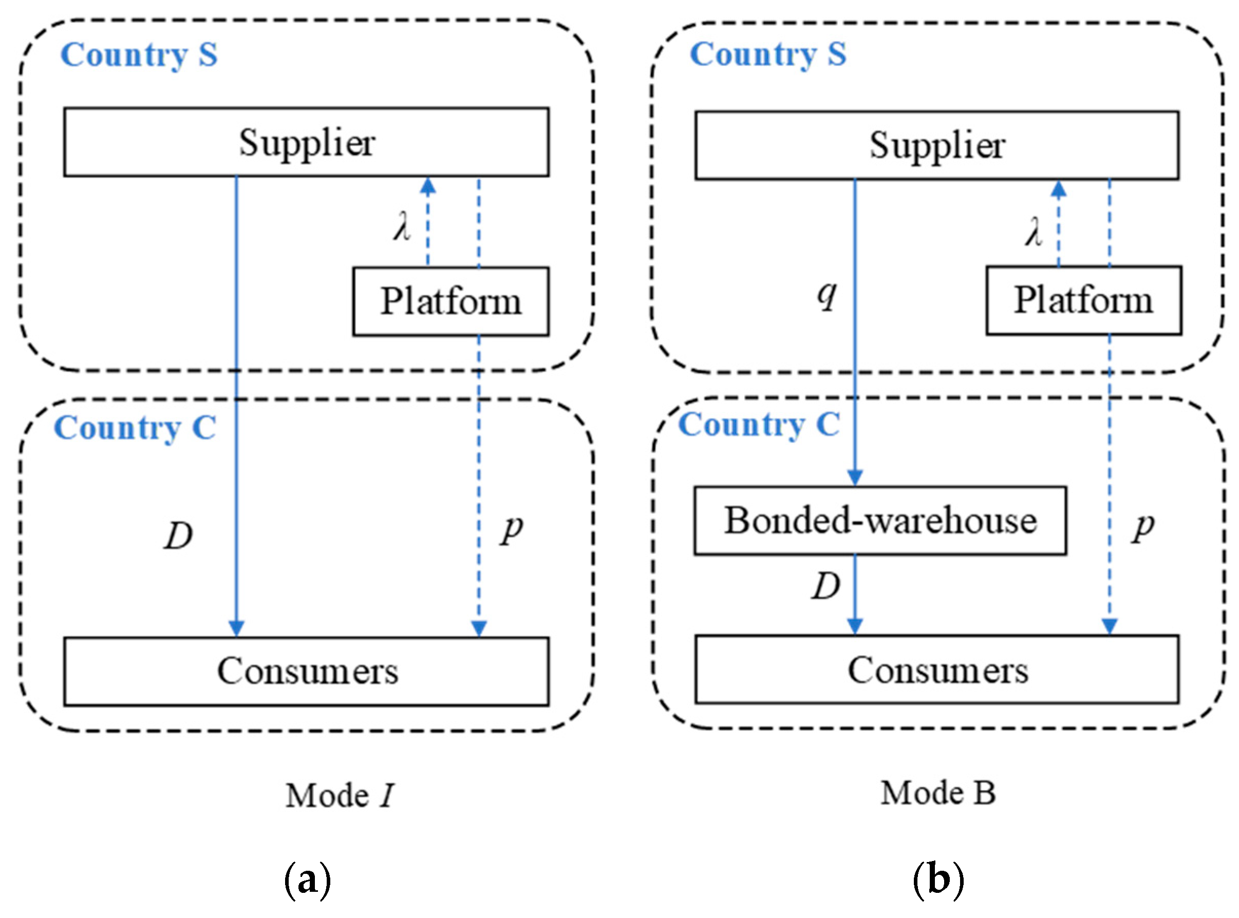
3. Model Description

Consider a supply chain consisting of a supplier and a CBEC platform. The supplier sells products directly to overseas consumers through the platform and pays a commission of $\lambda$ of the revenue. The platform commission is a percentage of the revenue and is an exogenous variable. This assumption aligns with the commercial practice of CBEC platforms and is widely adopted in the literature [3,9,57]. Commercial data indicates that on Amazon, the standard commission rate varies from 6% to 25% of the sales price, depending on the product category. On Tmall Global, the sales commission is typically calculated based on the price, type, and transaction amount of the goods, ranging from 2% to 5%. The average sales commission on AliExpress is approximately 5–8% [58].

The supplier can choose between two logistics modes, direct mail, and a bonded warehouse, to deliver products to consumers. In the direct mail mode, the supplier receives the online order from the consumer and delivers the product directly from the local warehouse internationally to the overseas consumer. If the bonded warehouse model is chosen, the supplier needs to decide in advance about the amount $q$ of stock to be prepared in the overseas warehouse. The stock quantity $q$ is shipped to the overseas warehouse in the overseas market. During formal sales, products are directly delivered from the bonded warehouse to the consumer after the order is received. For convenience, this paper refers to the direct mail mode as “mode I,” as shown in Figure 1a, and the bonded warehouse logistics mode as “mode B,” as shown in Figure 1b.

The supplier and consumers are located in country $S$ and country $C$, respectively, with the supplier’s currency denoted as $S$ and the consumers’ currency as $C$. Consumers purchase the supplier’s products through the CBEC platform and place orders in currency $C$ through a third-party payment platform, which periodically settles the exchange into currency $S$ and transfers it to the supplier’s account. During this period, the exchange rate fluctuates in both directions, exposing the supplier to exchange rate transaction risk (transaction risk refers to the possibility of loss due to exchange rate changes in transactions denominated in foreign currencies). Assume the exchange rate between $S$ and $C$ countries is $x_0$, representing the exchange rate at the beginning of the sales season (i.e., 1 unit of country $C$ can be exchanged for $x_0$ units of country $S$). Since settlement in foreign exchange takes time, the future exchange rate $X$, which is a random variable, may differ from $x_0$. If the currency of country $S$ appreciates or the currency of country $C$ depreciates, $X$ decreases, and vice versa.

The supplier’s unit production cost is denoted as $c$ in the currency $S$, represented as $c\left(S\right)$. The market price of the product is $p$ in the currency $C$, represented as $p\left(C\right)$, and is converted into the currency of the country $S$ at the time of settlement, resulting in an actual unit revenue of $Xp$ for the supplier. It is assumed that the tax is already included in the selling price and is the same under the two logistic modes [3,9]. This assumption allows us to better focus on exchange rate uncertainty. In the paper, overseas market demand is assumed to be a random variable, denoted by $D$. In addition, the actual exchange rate $X$ at the time of settlement is also a random variable. Due to the supplier’s distance from the overseas market, it is challenging to obtain accurate market distribution information, and only the first and second-moment information of $D$ and $X$ is available. These parameters are given by the matrix $\sum$.

$$\sum =\left(\begin{array}{ccc}E\left(X^2\right)& E\left(XD\right)& E\left(X\right)\\ E\left(XD\right)& E\left(D^2\right)& E\left(D\right)\\ E\left(X\right)& E\left(D\right)& 1\end{array}\right)$$

(1)

Define (1) as the moment matrix. Since $X,D>0$, the matrix $\sum$ is a semipositive definite matrix. Let $\mathsf{\Phi }\left({\sum }_0\right)=\left\{\left(\mathrm{X}, \mathrm{D}\right); \mathrm{X}, \mathrm{D}>0, \mathrm{exists} \mathrm{X}, \mathrm{D} \mathrm{satisfying}{\sum }_0=\sum \right\}$. All decisions are derived from the worst-case distribution in $\mathsf{\Phi }\left({\sum }_0\right)$. That is, the first and second-moment information of the exchange rate and demand, $E\left(X\right),E\left(D\right),E\left(X^2\right),E\left(D^2\right),\mathrm{a}\mathrm{n}\mathrm{d} E\left(XD\right)$, are extracted from ${\sum }_0$.

Table 2. Model notations.

Notation	Description
$\lambda$	$\lambda \in \left(\mathrm{0,1}\right)$, the commission rate paid by the supplier to the platform
$q$	Suppliers’ overseas warehouse stock quantity (decision variable)
$p\left(C\right)$	Unit product selling price
$c\left(S\right)$	Unit product cost
$c_B\left(S\right)$	Supplier’s unit logistics cost under the bonded warehouse mode
$c_I\left(S\right)$	Supplier’s unit logistics cost under the direct mail mode
$\psi$	$\psi =c_B/c_I,\psi \in \left(\mathrm{0,1}\right)$, denotes the logistics cost advantage of the bonded warehouse mode
$x_0$	The exchange rate at the beginning of the selling season: 1 unit of currency in country $C$ can be exchanged for $x_0$ units of currency in country $S$
$X$	The exchange rate at the time of settlement by the supplier: 1 unit of currency in country $C$ can be exchanged for $X$ units of currency in country $S$

summarizes the main symbols used throughout the study.

3.1. Bonded Warehouse Mode

When the supplier chooses mode B, they need to make a decision in advance about the amount of inventory $q$ to be stocked in the overseas warehouse, shipping the products to the overseas warehouse before the sales season begins. The supplier faces random market demand $D$, and only the demand of $min\left[q,D\right]$ can be satisfied. If $q<D$, there is a risk of out-of-stock. If $q>D$, there is a surplus of inventory. Without loss of generality, the residual value of leftover inventory is treated as zero, a common approach in many studies [9,59,60]. Under mode B, the supplier’s unit logistics cost is $c_B\left(S\right)$, including transportation and labor costs borne by the supplier. The supplier needs to pay $\lambda$ proportion of the sales revenue to the platform. Thus, the supplier’s expected profit (in the currency of country $S$) is:

$${\pi }_B\left(q\right|X,D)=E_{X,D}\left\{\left(1-\lambda \right)\left[XpEmin\left(q,D\right)\right]\right\}-\left(c+c_B\right)q$$

(2)

The first term on the right side of Equation (2) represents the actual sales revenue after deducting the commission, and the second term represents the total cost. In mode B, the problem faced by the supplier is to maximize the expected profit under the worst-case scenario by providing the optimal overseas warehouse stock quantity $q$. Therefore, the supplier’s profit function (2) is transformed into the following robust newsvendor problem:

$$\underset{q\ge 0}{\mathit{max}}\underset{\left(X,D\right)\in {\sum }_0}{\mathit{inf}}{\pi }_B\left(q\right|X,D)$$

(3)

Theorem 1 below provides the optimal stock quantity and profit of the supplier under mode B.

Theorem 1. 

The optimal stocking quantity of the supplier’s overseas warehouse is:

$$q*=\left\{\begin{array}{c}E\left(D\right)+{\displaystyle \frac{\alpha }{\sqrt{K}}}\sigma \left(D\right), M\le N\\ 0, M>N\end{array}\right.$$

(4)

In this case, the supplier’s expected profit in the worst-case scenario is:

$${\mathrm{\Pi }}_{wst}=\alpha E\left(D\right)-\sqrt{K}\sigma \left(D\right)+{\displaystyle \frac{1}{2}}\left(1-\lambda \right)pE\left(XD\right)$$

(5)

where $E\left(·\right)$ denotes the mean and $\sigma \left(·\right)$ denotes the standard deviation. Besides, $\alpha ={\displaystyle \frac{1}{2}}\left(1-\lambda \right)pE\left(X\right)-\left(c+\psi c_I\right)$, $\beta ={\displaystyle \frac{1}{4}}{\left(1-\lambda \right)}^2{p}^{2}E\left(X^2\right)$, $K=\beta -{\alpha }^2={\displaystyle \frac{1}{4}}{\left(1-\lambda \right)}^2{p}^2{\sigma }^2\left(X\right)+\left(1-\lambda \right)pE\left(X\right)\left(c+\psi c_I\right)-{\left(c+\psi c_I\right)}^2$, ${M=\left[E\left(D^2\right)-qE\left(D\right)\right]}^{2}E\left(X^2\right)$, ${N=E}^2\left(XD\right)\left[q^2-2qE\left(D\right)+E\left(D^2\right)\right]$.

Proof of Theorem 1. 

The proof process is shown in Appendix A.1. □

3.2. Direct Mail Mode

When the supplier chooses mode I, they can arrange the supply of products in time after receiving the orders from the consumers, thus meeting all market demands with no inventory risk. However, under mode I, each order needs to be shipped from country $S$ to country $C$, resulting in higher logistics costs $c_I\left(S\right)$. Therefore, it is assumed that the logistics cost under mode I is higher than mode B [9], i.e., $c_I>c_B$, which aligns with commercial practice. For model analysis, let $c_B=\psi c_I$, where $\psi \in \left(\mathrm{0,1}\right)$ represents the logistics cost advantage of mode B. The lower the $\psi$, the greater the logistics cost advantage of mode B. Under mode I, the supplier’s expected profit is:

$${\pi }_I\left(X,D\right)=\left(1-\lambda \right)pE\left(XD\right)-\left(c+c_I\right)E\left(D\right)$$

(6)

The first term on the right side of Equation (6) represents the actual sales revenue after deducting the commission ratio, and the second term represents the total production and logistics costs. Since every order can be fulfilled under mode I, there is no inventory decision, and Equation (6) is the supplier’s expected profit.

4. Analysis

In this section, based on the mode setup and solution in Section 3, we first analyze the main factors affecting the supplier’s optimal inventory decision and profit under mode B. Secondly, we compare supplier profits under both logistics modes, focusing on how market demand, exchange rate appreciation and depreciation, demand volatility, exchange rate fluctuations, the correlation between exchange rate and demand, and logistics costs influence the supplier’s logistics mode choice.

4.1. Optimal Inventory Analysis for Mode B

This subsection discusses the impact of $E\left(X\right),E\left(D\right),\sigma \left(D\right),\sigma \left(X\right),\lambda ,\psi$, and $p$ on the optimal stocking quantity as well as profit under mode B.

Proposition 1. 

(i) 

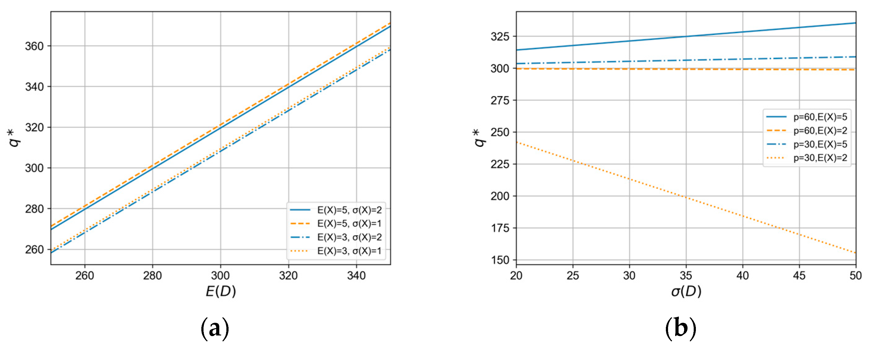
When the constraint $M\le N$   is satisfied, the optimal stocking quantity  $q*$  increases monotonically with the mean value of demand $E\left(D\right)$. The monotonicity of  $q*$ with $\sigma \left(D\right)$ depends on $\alpha$. Specifically, if  $\alpha >0$, $q*$ increases with $\sigma \left(D\right)$. If $\alpha <0$, $q*$ decreases with $\sigma \left(D\right)$.

(ii) 

When the constraint $M\le N$ is satisfied, the supplier’s profit ${\pi }_B$ under mode B varies with the mean value of demand $E\left(D\right)$ also depends on $\alpha$. If $\alpha >0$, ${\pi }_B$ increases with $E\left(D\right)$, if $\alpha <0$, ${\pi }_B$ decreases with $E\left(D\right)$. Supplier profit ${\pi }_B$ under mode B monotonically decreases with the standard deviation of demand $\sigma \left(D\right)$.

Proof of Proposition 1. 

The proof process is shown in Appendix A.2. □

The mean value of demand represents the average number of overseas consumers purchasing products through the e-commerce platform. The larger the average demand, the more consumers there are, and the supplier needs to increase the inventory in the overseas warehouse to meet the higher market demand. The standard deviation of market demand reflects the degree of market volatility. A higher standard deviation represents greater market volatility. When market demand volatility increases, the adjustment of the stock quantity depends on the profit margin of the product. $\left(1-\lambda \right)pE\left(X\right)$ represents the actual revenue per unit product in the currency $S$, while $c+c_B$ represents the total cost per unit product. $\alpha >0$ means $\left(1-\lambda \right)pE\left(X\right)>2\left(c+c_B\right)$, indicating that the actual revenue exceeds twice the cost, characterizing the product as high profit. Suppliers will increase the inventory of high-profit products in the overseas warehouse to meet additional demand due to market volatility and reduce inventory for low-profit products in response to potential demand decreases.

In mode B, the impact of average market demand on suppliers’ profit also depends on the profit margin of the products. When selling high-profit products, increased average market demand will boost the supplier’s profit. On the contrary, when selling low-profit products, higher market demand may reduce overall profit, so suppliers should emphasize the profitability indexes in commodity selection. When the uncertainty of overseas market demand increases, it will reduce the overall profit of suppliers, which is consistent with the findings of existing studies [54,61].

Proposition 2. 

(i) 

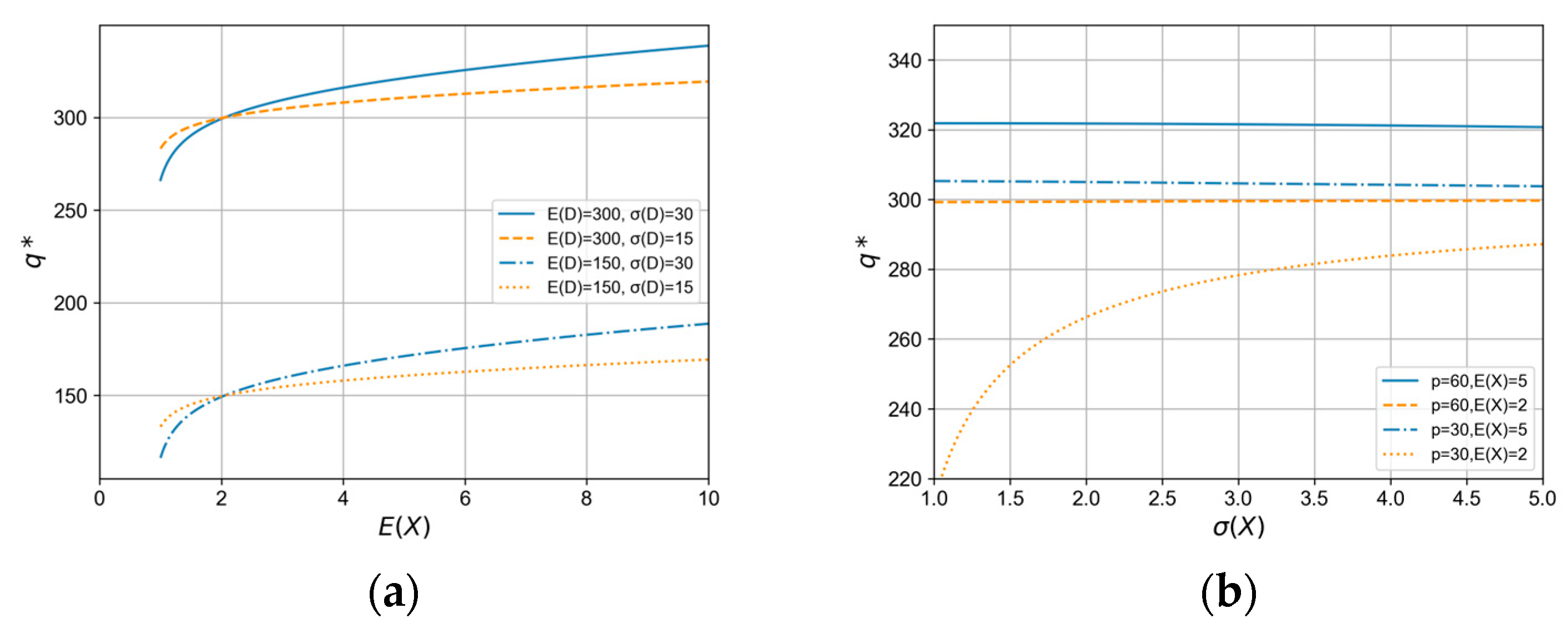
When the constraint $M\le N$ is satisfied, the optimal stocking quantity $q*$ increases monotonically with the mean value of the exchange rate $E\left(X\right)$. The monotonicity of $q*$ with respect to $\sigma \left(X\right)$ depends on $\alpha$, if $\alpha >0$, $q*$ decreases with $\sigma \left(X\right)$, if $\alpha <0$, $q*$ increases with $\sigma \left(X\right)$.

(ii) 

When the constraint $M\le N$ is satisfied, ${\pi }_B$ is a convex function of $E\left(X\right)$ and decreases monotonically with $\sigma \left(X\right)$.

Proof of Proposition 2. 

The proof process is shown in Appendix A.3. □

$X$ represents the actual exchange rate when the supplier settles, where 1 unit of currency in country $C$ can be exchanged for $X$ units of currency in country $S$. The mean value of the exchange rate $E\left(X\right)$ represents the average exchange ratio between the two currencies. When $E\left(X\right)$ increases, the supplier’s currency depreciates, and the consumer’s currency appreciates. Conversely, when $E\left(X\right)$ decreases, the supplier’s currency appreciates, and the consumer’s currency depreciates. When the mean value of the exchange rate increases, currency depreciation in the supplier’s country favors exports, so suppliers increase overseas warehouse inventory to meet the overseas market. $\sigma \left(X\right)$ is the standard deviation of exchange rate volatility, measuring the degree of exchange rate fluctuation. The impact of exchange rate volatility on overseas warehouse inventory depends on the product’s profit margin. Suppliers reduce high-profit overseas warehouse inventory and increase low-profit product inventory to cope with more significant exchange rate fluctuations. Comparing Proposition 1, suppliers adopt differentiated inventory strategies to respond to demand and exchange rate risks, increasing high-profit products to address market volatility and low-profit products to address exchange rate volatility.

The impact of the mean value of the exchange rate on the supplier’s profit decreases first and then increases. As $E\left(X\right)$ increases, currency depreciation in the supplier’s country initially reduces profit, then increases it. When the depreciation exceeds a certain threshold, the increase in export volume compensates for the exchange loss, leading to higher overall profit. When currency depreciation reaches a certain degree, the export benefits can offset the exchange loss, enhancing the supplier’s overall profit.

Proposition 3. 

(i) 

When the constraint $M\le N$ is satisfied, the optimal inventory level $q*$ decreases monotonically with $\lambda$ and $\psi$, but increases monotonically with $p$.

(ii) 

When the constraint $M\le N$ is satisfied, the supplier’s profit ${\pi }_B$ is a convex function of $\lambda$, $\psi$, and $p$.

Proof of Proposition 3. 

The proof process is shown in Appendix A.4. □

Proposition 3 analyzes the impact of unit product cost advantage and selling price on overseas warehouse inventory levels. The supplier needs to pay $\lambda$ proportion of revenue as a platform commission. A higher commission ratio means lower profit per unit product, so suppliers reduce inventory to minimize losses. $\psi$ represents the logistics cost advantage of mode B compared to mode I. A higher $\psi$ indicates a lower logistics cost advantage, reducing overseas warehouse inventory. As the unit product market price $p$ increases, the supplier’s unit profit increases, leading to higher overseas warehouse inventory to gain more profit.

4.2. Logistics Mode Analysis

Comparing supplier profits under mode I and mode B, we analyze how exchange rate appreciation and depreciation, exchange rate volatility, the mean value of market demand, demand volatility, the covariance between exchange rate and demand, and logistics costs influence logistics mode choice. Specifically, this section discusses the impact of $E\left(X\right),E\left(D\right),\sigma \left(D\right),\sigma \left(X\right),cov(X,D)$, and $\psi$ on the choice between the two logistics modes.

Proposition 4. 

(i) 

When the constraint $M\le N$ is satisfied, if $E\left(D\right)<E_1\left(D\right)$, ${\pi }_B<{\pi }_I$. If $E\left(D\right)>E_1\left(D\right)$, ${\pi }_B>{\pi }_I$. Where $E_1\left(D\right)={\displaystyle \frac{\sqrt{K}\sigma \left(D\right)+1/2\left(1-\lambda \right)pcov(X,D)}{\left(1-\psi \right)c_I}}$.

(ii) 

When the constraint $M\le N$ is satisfied, if $\sigma \left(D\right)<{\sigma }_1\left(D\right)$, ${\pi }_B>{\pi }_I$. If $\sigma \left(D\right)>{\sigma }_1\left(D\right)$, ${\pi }_B<{\pi }_I$. Where ${\sigma }_1\left(D\right)={\displaystyle \frac{\left(1-\psi \right)c_{I}E\left(D\right)-1/2\left(1-\lambda \right)pcov(X,D)}{\sqrt{K}}}$.

Proof of Proposition 4. 

The proof process is shown in Appendix A.5. □

From Proposition 4, the level of market demand affects the choice of logistics mode of CBEC suppliers. $E\left(D\right)<E_1\left(D\right)$ indicates relatively low market demand, prompting suppliers to choose mode I, increasing logistics costs, and reducing inventory. Correspondingly, $E\left(D\right)>E_1\left(D\right)$ indicates relatively high market demand, leading suppliers to choose mode B, prestocking inventory in the consumer’s country. When $\sigma \left(D\right)<{\sigma }_1\left(D\right)$, market demand volatility is relatively low, and suppliers choose mode B to supply a relatively stable market. When $\sigma \left(D\right)>{\sigma }_1\left(D\right)$, high market demand volatility necessitates mode I to avoid significant inventory risk. This conclusion is consistent with existing research [3,9].

Proposition 5. 

(i) 

Satisfying the constraint $M\le N$, the effect of the mean value of the exchange rate $E\left(X\right)$ on the logistics mode needs to be discussed in separate cases:

• Case 1. When $\psi <{\psi }_1$, we can obtain ${\pi }_B>{\pi }_I$ no matter how the mean value of the exchange rate changes.
• Case 2. When $\psi >{\psi }_1$, ${\pi }_B>{\pi }_I$ if $E\left(X\right)<E_0\left(X\right)$, or if $E\left(X\right)>E_2\left(X\right)$.
• Case 3. If $E_0\left(X\right)<E\left(X\right)<E_2\left(X\right)$, ${\pi }_B<{\pi }_I$.
• Where

  $$E_0\left(X\right)={\displaystyle \frac{2\left(1-\lambda \right)p{\sigma }^2\left(D\right)\left(c+\psi c_I\right)-2\sqrt{G}}{{\left(1-\lambda \right)}^2{p}^2{\sigma }^2\left(D\right)}}, E_2\left(X\right)={\displaystyle \frac{2\left(1-\lambda \right)p{\sigma }^2\left(D\right)\left(c+\psi c_I\right)+2\sqrt{G}}{{\left(1-\lambda \right)}^2{p}^2{\sigma }^2\left(D\right)}}.$$

  $${\psi }_1={\displaystyle \frac{c_{I}E\left(D\right)-1/2\left(1-\lambda \right)p\left[cov\left(X,D\right)+\sigma \left(D\right)\sqrt{E\left(X^2\right)}\right]}{c_{I}E\left(D\right)}}, G={\left[\left(1-\lambda \right)p{\sigma }^2\left(D\right)\left(c+\psi c_I\right)\right]}^2+{\left(1-\lambda \right)}^2{p}^2{\sigma }^2\left(D\right)\left[{\displaystyle \frac{1}{4}}{\left(1-\lambda \right)}^2{p}^2{\sigma }^2\left(D\right)E\left(X^2\right)-{(c+\psi c_I)}^2-{\left(\left(1-\psi \right)c_{I}E\left(D\right)-{\displaystyle \frac{1}{2}}\left(1-\lambda \right)pcov\left(X,D\right)\right)}^2\right].$$

(ii) 

Satisfying the constraint $M\le N$, when $\sigma \left(X\right)<{\sigma }_1\left(X\right)$, ${\pi }_B>{\pi }_I$. When $\sigma \left(X\right)>{\sigma }_1\left(X\right)$, ${\pi }_B<{\pi }_I$.

Proof of Proposition 5. 

The proof process is shown in Appendix A.6. □

The impact of the mean value of the exchange rate on the supplier’s logistics mode depends not only on the appreciation and depreciation of the exchange rate but also on the trade-off of logistics costs between the two modes. When $\psi <{\psi }_1$, the cost advantage of mode B is relatively significant, and suppliers will ignore the changes in exchange rates between the two countries and always choose mode B with superior logistics costs. When $\psi >{\psi }_1$, the cost advantage of mode B gradually decreases, and suppliers will balance exchange rate fluctuations to choose the logistics mode. Specifically, when the currency of the supplier’s country appreciates or depreciates significantly, mode B can yield higher profits. When the exchange rate remains stable within a specific range, suppliers should choose mode I.

When $\sigma \left(X\right)<{\sigma }_1\left(X\right)$, i.e., the exchange rate fluctuations are relatively small, suppliers choose mode B. Conversely, when exchange rate fluctuations are relatively large, suppliers choose mode I. Proposition 5 clearly shows that exchange rate fluctuations have a significant impact on the supplier’s logistics mode choice, something that has not been considered in previous literature [15]. Specifically, exchange rate fluctuations influence the supplier’s overseas warehouse inventory decisions, thereby affecting profits under different logistics modes. Existing research has found that when demand fluctuates wildly, suppliers will adopt mode I to reduce inventory risk [9]. This paper, on this basis, further finds that when exchange rate fluctuations increase, suppliers will also choose mode I to cope with exchange rate risk. Therefore, mode I can also mitigate the exchange rate fluctuation risk while reducing the inventory risk.

Proposition 6. 

Satisfying the constraint $M\le N$, the effect of the covariance $cov(X,D)$ on the logistics mode needs to be discussed in separate cases:

• Case 1: When $\psi \le {\psi }_2$, if $cov(X,D)>{cov}_1(X,D)$, $X$ and $D$ are positively correlated, ${\pi }_B<{\pi }_I$.
• Case 2: When $\psi <{\psi }_2$, if $cov(X,D)<{cov}_1(X,D)$, the correlation between $X$ and $D$ changes from positive to negative, ${\pi }_B>{\pi }_I$.
• Case 3: When $\psi >{\psi }_2$, if cov $cov(X,D)>{cov}_1(X,D)$, the correlation between $X$ and $D$ changes from negative to positive, ${\pi }_B<{\pi }_I$.
• Case 4: When $\psi \ge {\psi }_2$, if $cov(X,D)<{cov}_1(X,D)$, $X$ and $D$ are negatively correlated, ${\pi }_B>{\pi }_I$.
• Where ${\psi }_2=1-{\displaystyle \frac{\sqrt{K}\sigma \left(D\right)}{c_{I}E\left(D\right)}}$, ${cov}_1\left(X,D\right)={\displaystyle \frac{2\left(1-\psi \right)c_{I}E\left(D\right)-2\sqrt{K}\sigma \left(D\right)}{\left(1-\lambda \right)p}}$.

Proof of Proposition 6. 

The proof process is shown in Appendix A.7. □

Covariance represents the correlation between two variables, and $cov(X,D)$ measures the correlation between the uncertain exchange rate $X$ and demand $D$. According to Proposition 6, when the correlation between the two random variables exceeds a certain threshold (high correlation), the supplier’s profit under mode I is always higher than mode B, prompting suppliers to choose mode I. When the correlation between the two random variables is below a certain threshold (low correlation), suppliers choose mode B. In addition, the logistics costs of the two modes change the direction of the correlation between exchange rate and demand. $\psi <{\psi }_2$ indicates a more significant cost advantage of mode B. As the cost advantage increases, the correlation between exchange rate and demand gradually changes from positive to negative. $\psi >{\psi }_2$ indicates a smaller cost advantage of mode B, and the correlation between exchange rate and demand changes from negative to positive.

The impact of exchange rate changes on market volatility can be observed in various products and industries. When the correlation between exchange rate and demand is high, exchange rate fluctuations can quickly affect demand, such as in luxury goods and electronics. For example, the devaluation of the Yen in 2024 increased demand for luxury goods [62]. At this time, suppliers may prefer mode I to respond directly to demand changes and seize sales opportunities quickly. When the correlation between exchange rate and demand is low, consumer purchasing behavior is less affected by exchange rate fluctuations, and demand remains relatively stable, such as in essential goods and pharmaceuticals. In this case, adopting mode B can provide more stable supply chain management and act as a buffer against exchange rate fluctuations.

Table 3. The impact of exchange rate and demand on logistics mode choices.

Main Factors	Trend	Logistics Mode Choice
Mean value of demand	Low market demand	Mode I
	High market demand	Mode B
Demand volatility	Low market volatility	Mode B
	High market volatility	Mode I
Mean value of exchange rate	The logistics cost advantage of mode B is significant	Mode B
	The logistics cost advantage of mode B is minimal and the mean value of the exchange rate is too low or too high	Mode B
	The logistics cost advantage of mode B is minimal, and the mean value of the exchange rate remains stable within a certain threshold	Mode I
Exchange rate volatility	Low exchange rate volatility	Mode B
	High exchange rate volatility	Mode I
Exchange rate and demand correlation	High correlation	Mode I
	Low correlation	Mode B

summarizes the impact of significant factors on suppliers’ choice of logistics mode.

5. Numerical Studies

In this section, we first use numerical studies to analyze the impact of crucial model parameters on the optimal inventory level under mode B. Then, we compare the optimal profits of suppliers under two logistics modes, analyzing the main factors affecting the mode selection. Finally, we conduct a robustness analysis of the overseas warehouse inventory strategy by comparing supplier profits under partial and complete demand distribution information.

Without losing generality, we consider the following scenario: a supplier sells products to overseas consumers through a CBEC platform. The unit selling price is $p\left(C\right)=60$, the production cost is $c\left(S\right)=40$, and the supplier pays the platform $\lambda =0.06$ of the revenue as a commission. According to the commission rates charged by Amazon (6–25%) and AliExpress (5–8%), this paper selects 6% as the platform commission rate. The supplier delivers goods through two logistics modes, Mode B and Mode I. The logistics cost under mode I is $c_I\left(S\right)=20$, and under Mode B, it is $c_B\left(S\right)=\psi c_I=18$. Here, $\psi =0.9$ indicates the relative logistics cost advantage of Mode B [9]. In addition, under Mode B, the supplier needs to ship the products to the overseas warehouse before sales, facing a random market demand $D$. Suppose the mean value of the random market demand is $E\left(D\right)=300$, and the standard deviation is $\sigma \left(D\right)=30$ [53,54]. At the end of the sales period, the supplier needs to convert the total revenue in foreign currency into domestic currency, facing a random exchange rate $X$. The mean value of the exchange rate $E\left(X\right)=5$, and the standard deviation $\sigma \left(X\right)=1$. The random demand and exchange rate have a correlation term $E\left(XD\right)=0$ [3,54]. The values are used in the numerical studies in this section unless otherwise stated.

5.1. Analysis of Mode B

First, we analyze the impact of the mean and variance of market demand on the optimal inventory level for mode B. Set $E\left(D\right)\in \left(\mathrm{250,350}\right)$ and $\sigma \left(D\right)\in \left(\mathrm{20,50}\right)$. Figure 2 shows that as the mean value of market demand increases, the supplier will always increase the overseas order quantity to meet market demand. When the mean value of the exchange rate is high, the supplier’s currency depreciates, which is more favorable for exports, leading to higher inventory levels. The impact of demand volatility on overseas warehouse inventory. $pE\left(X\right)$ represents the supplier’s unit revenue after conversion. When the total cost per unit product is fixed, a higher $pE\left(X\right)$ means a higher profit per unit product. When demand volatility increases, suppliers will increase the inventory of high-profit products and reduce the inventory of low-profit products to cope with market changes.

Next, we analyze the impact of the mean and variance of the exchange rate on the optimal inventory level for mode B. Set $E\left(X\right)\in \left(\mathrm{0,10}\right)$ and $\sigma \left(X\right)\in \left(\mathrm{1,5}\right)$. The mean value of the exchange rate represents the exchange rate between two countries. A higher mean implies a depreciation of the supplier’s currency. According to Figure 3a, as the currency depreciates, the supplier will increase export inventory, which aligns with business realities. The impact of exchange rate volatility on inventory also depends on the profitability of the product. In Figure 3b, the profitability of the product is changed by adjusting the unit selling price. When exchange rate volatility increases, suppliers will choose to increase low-profit products and decrease high-profit products to cope with exchange rate fluctuations. The degree of exchange rate volatility directly affects the size of the supplier’s exchange gains and losses, and increasing low-profit products can reduce the total revenue loss caused by high exchange rate volatility.

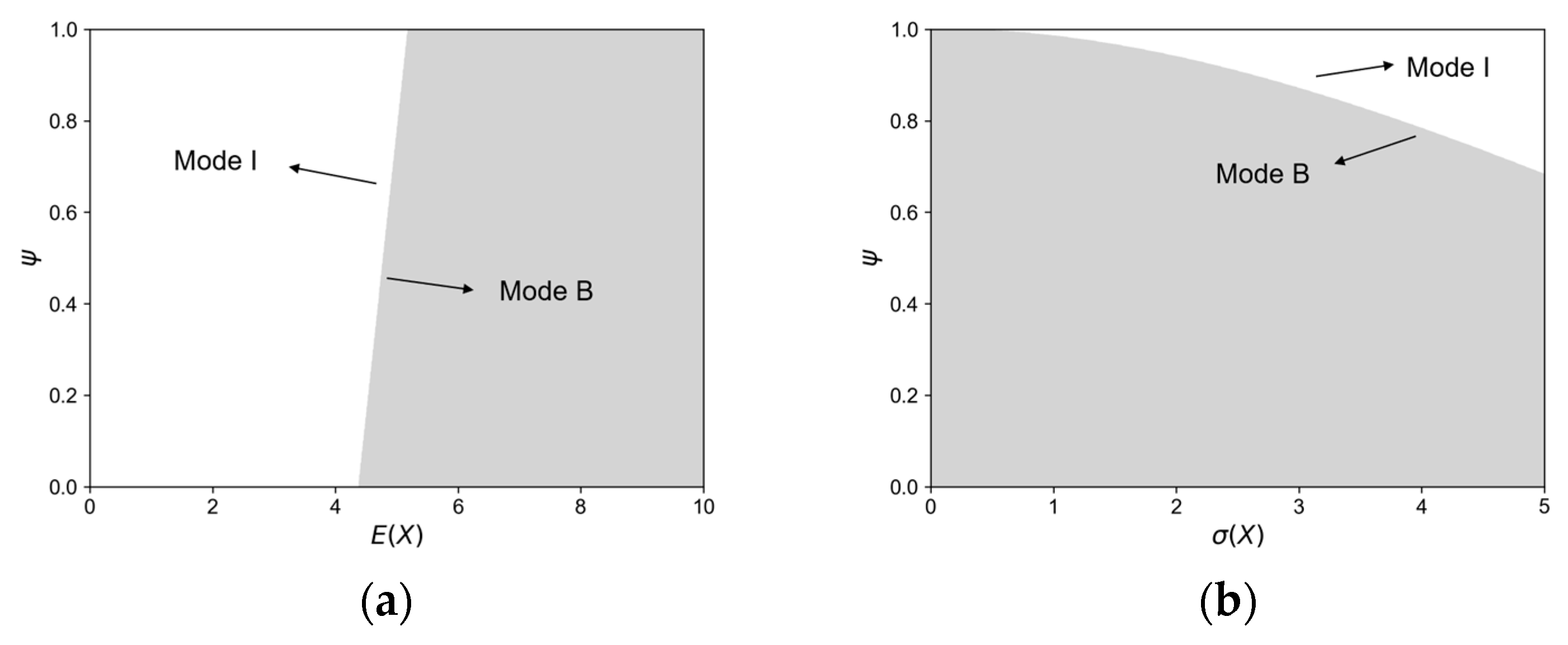
5.2. Comparison of Logistics Modes

This subsection analyzes the impact of the means, variances, covariances of demand and exchange rates, and logistics cost ratios on supplier profits under the two logistics modes. Figure 4a reflects the choice of logistics mode under the influence of two factors: the mean value of the exchange rate and the logistics cost ratio. Let $E\left(X\right)\in \left(\mathrm{0,10}\right)$ and $\psi \in \left(\mathrm{0,1}\right)$. Under the given constraints, when the mean value of the exchange rate exceeds a certain threshold, suppliers tend to choose mode B, which is the same as the second conclusion of Proposition 5. This is because when the supplier’s currency depreciates, it benefits exports, leveraging the logistics cost advantage of mode B. Figure 4b reflects the choice of logistics mode under the influence of two factors: exchange rate standard deviation and logistics cost ratio. Let $\sigma \left(X\right)\in \left(\mathrm{0,5}\right)$ and $\psi \in \left(\mathrm{0,1}\right)$. Under the given constraints and parameter settings, the choice of supplier logistics mode depends not only on exchange rate fluctuations but also on the trade-off of two logistics costs. When the cost advantage of mode B is significant, suppliers will choose mode B to reduce costs. However, when the logistics cost difference between the two modes narrows, suppliers will choose mode I to be more flexible to cope with market risk. In addition, when the exchange rate fluctuation increases, suppliers tend to choose mode I to deal with exchange rate risk.

Next, we analyze the impact of the mean and standard deviation of demand on logistics mode choice, with $E\left(D\right)\in \left(\mathrm{250,350}\right)$ and $\sigma \left(D\right)\in \left(\mathrm{0,80}\right)$. As shown in Figure 5a, when demand is relatively low, mode I is more cost-efficient for suppliers. As the mean value of demand increases, suppliers choose mode B to save logistic costs. Figure 5b shows the impact of demand standard deviation and logistics cost on the choice of supplier logistics mode. When demand volatility is high, mode I can more flexibly respond to rapid changes in demand, while a stable demand environment is more suitable for mode B. Figure 6 analyzes the impact of covariance on logistics mode choice. When $cov(X,D)\in (-1000, 1000)$, under the given parameters, mode B is chosen when the covariance is below a certain threshold, while mode I is chosen when it exceeds a certain range. Choosing mode I, when the covariance is high, is probably because it can quickly adapt to market dynamics when exchange rate and demand changes are synchronized. When the covariance is low or negative, mode B offers better cost control and risk management.

5.3. Impact of Partial Distribution Information on Optimal Results

Theorem 1 provides the supplier’s robust inventory decision for overseas warehouses when selling through a CBEC platform. This subsection conducts a robustness analysis of the overseas warehouse inventory strategy under random factors of demand and exchange rates. Specifically, we examine the profit differences between suppliers with only partial distribution information and those with accurate distribution information. This profit difference is also known as the expected value of additional information (EVAI) [41,54], which is the maximum amount a decision-maker is willing to pay to obtain accurate distribution information. In addition, we analyze the impact of exchange rate and demand volatility (standard deviation) on the EVAI of inventory levels. Existing research indicates that the performance of distributionally robust decisions is closer to that under a normal distribution [50,54], so this research assumes that the distributions of exchange rates and demand under complete information follow a normal distribution.

First, we present the supplier’s decisions and profits under normal distribution and compare the robustness with robust decisions. Let $X~N\left(5,1^2\right)$ and $D~N\left(300,{30}^2\right)$, where “$N$“ indicates that the random variable follows a normal distribution. Other variables are assumed as follows: $p\left(C\right)=120, c\left(S\right)=40,\lambda =0.06,c_I\left(S\right)=20,c_B\left(S\right)=\psi c_I=18$. At this time, $\mathrm{E}\mathrm{V}\mathrm{A}\mathrm{I}={{\pi }_N-\pi }_B$, representing the expected profit loss due to decisions made with only partial information. The profit difference ratio is ${({\pi }_N-\pi }_B)/{\pi }_B$, indicating the profit margin error between partial distribution information and normal distribution. Then, under the given parameters, we analyze the impact of exchange rate and demand volatility on EVAI. The results are shown in

Table 4. The suppliers’ optimal profits under different $\mathsf{\sigma }\left(X\right)$ and $\mathsf{\sigma }\left(D\right)$.

σ(X)	σ(D)	Optimal Profit (Normal Distribution)	Optimal Profit (Partial Distribution Information)	Profit Loss Ratio
2	5	159,845.01	133,109.30	20.09%
	10	163,612.02	132,178.61	23.78%
	15	167,379.03	131,247.91	27.53%
	20	171,146.04	130,317.21	31.33%
	25	174,913.06	129,386.52	35.19%
	30	178,680.07	128,455.82	39.10%
3	5	159,845.01	132,915.80	20.26%
	10	163,612.02	131,791.61	24.14%
	15	167,379.03	130,667.41	28.10%
	20	171,146.04	129,543.22	32.12%
	25	174,913.06	128,419.02	36.20%
	30	178,680.07	127,294.83	40.4%
4	5	159,845.01	132,690.75	20.46%
	10	163,612.02	131,341.49	24.57%
	15	167,379.03	129,992.24	28.76%
	20	171,146.04	128,642.99	33.04%
	25	174,913.06	127,293.73	37.41%
	30	178,680.07	125,944.48	41.87%
5	5	159,845.01	132,447.45	20.69%
	10	163,612.02	130,854.91	25.03%
	15	167,379.03	129,262.36	29.49%
	20	171,146.04	127,669.82	34.05%
	25	174,913.06	126,077.27	38.73%
	30	178,680.07	124,484.73	43.54%

.

From the results in Table 4, we can see that the supplier’s optimal expected profit under partial distribution information is always less than the optimal expected profit under normal distribution [49,54]. In this case, EVAI is always greater than zero, and suppliers must incur costs to obtain more accurate market information. In addition, as exchange rate volatility increases, the supplier’s profit under partial distribution information decreases, and the profit difference ratio with the normal distribution increases. This implies that as exchange rate volatility increases, the lack of distributional information leads to more profit loss for suppliers. Similarly, we find that as demand volatility increases, profits under partial distribution information decrease, and the profit difference ratio with the normal distribution increases. Demand volatility also leads to reduced profits due to missing distribution information. In other words, under partial information, excessive market or exchange rate volatility harms supplier profits.

6. Conclusions

6.1. Main Conclusions

Based on the rapid development of CBEC, this paper analyzes the logistics mode choice of suppliers selling through CBEC platforms. In a supply chain consisting of a supplier and a CBEC platform, the supplier sells products to overseas markets through the platform and pays a commission. The supplier can choose either mode I or mode B to deliver the products to consumers. This paper focuses on analyzing the impact of demand and exchange rate uncertainty on the supplier’s choice of logistics mode. To analyze the influence of demand and exchange rates, we assume that overseas market demand and exchange rate are both random, with the supplier knowing only partial distribution information, such as mean, variance, and covariance. The distributionally robust optimization method is used to give the decision of the optimal stocking quantity for overseas warehouses, and the following main conclusions are obtained by comparing the supplier’s profit under the two logistics modes of mode I and mode B:

(i)

The optimal inventory level for mode B increases monotonically with the mean value of demand and exchange rate. As market demand increases, suppliers increase their overseas warehouse inventory to meet higher market demand. The average exchange rate represents the average exchange rate of the two countries’ currencies, and an increase in the average exchange rate means that the currency of the supplier’s country depreciates, which is more favorable for export, so the supplier will increase the stocking quantity of overseas warehouses to satisfy the overseas market. The impact of demand and exchange rate volatility on the supplier’s overseas warehouse inventory depends on the product’s profit margin. Specifically, when demand volatility increases, suppliers increase high-profit products and decrease low-profit products. When exchange rate volatility increases, suppliers reduce high-profit products and increase low-profit products to cope with exchange rate risk.

(ii)

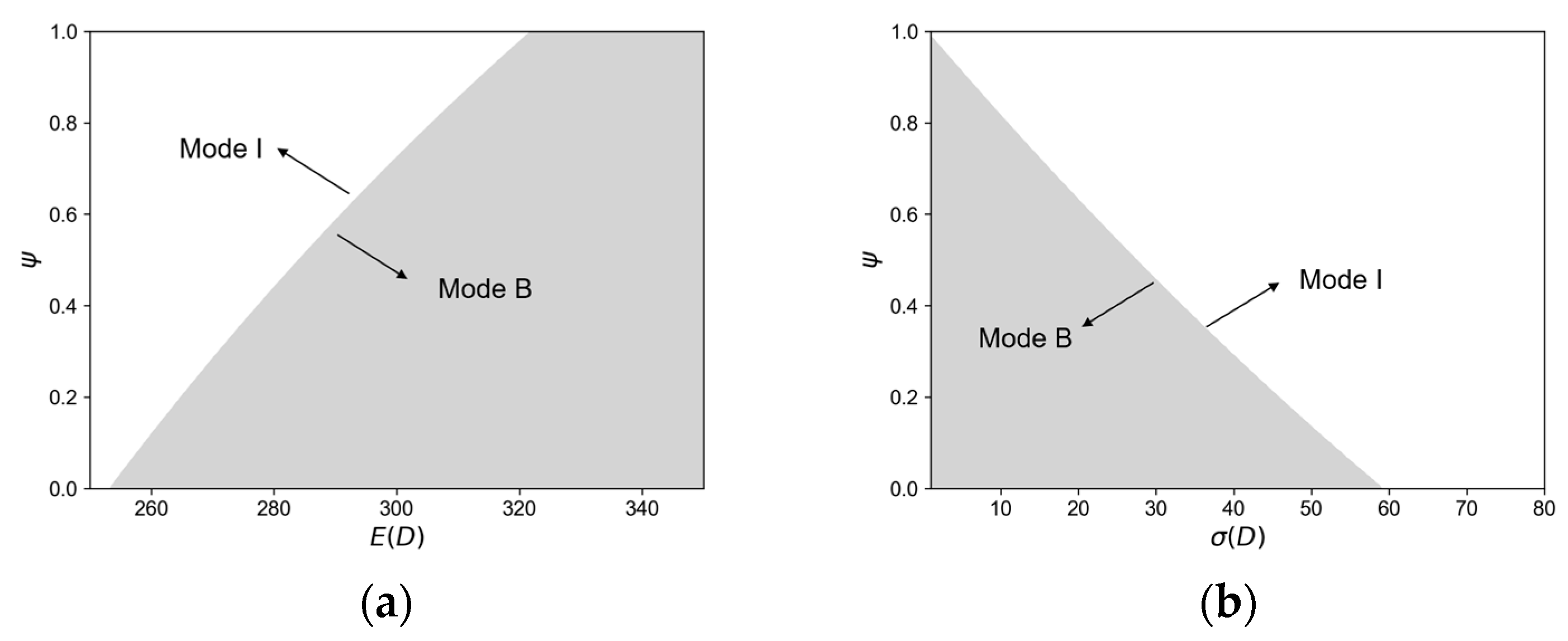
The levels of mean value of demand and exchange rate influence the supplier’s logistics mode choice. When market demand is low, mode I provides higher flexibility and lower operating costs, leading suppliers to prefer mode I. On the contrary, when the level of market demand is high, mode B becomes more economical. Centralized storage can reduce unit logistics costs and improve logistics efficiency, and suppliers prefer mode B. This conclusion is consistent with the current logistics practice. For instance, sellers of special handicrafts or custom-made goods on platforms like Etsy or Shopify typically tend to use mode I due to their smaller order volumes. Large CBEC platforms such as Tmall Global and JD International usually employ mode B to handle large volumes of orders. The impact of exchange rate averaging on the logistics mode also depends on the logistics cost trade-off. When the cost of mode B has a clear advantage, suppliers will always choose mode B. When the cost advantage of mode B decreases, if the exchange rate stabilizes within a specific range, suppliers will choose mode I; otherwise, they will choose mode B.

(iii)

There is consistency in the impact of exchange rate and market demand fluctuations on suppliers’ logistics mode. When both exchange rate and demand volatility are low, indicating a relatively stable market, suppliers can use mode B to optimize cost structure and improve overall supply chain efficiency. Conversely, when exchange rate and demand risks increase, market uncertainty rises. In this environment, mode I offers higher flexibility and quicker response capability, better adapting to demand and exchange rate fluctuations, leading suppliers to choose mode I. This finding is not only consistent with Zha et al. [9] and Zhang et al. [3] on the impact of demand fluctuations on logistics mode choice but also the first systematic exploration of the impact of exchange rate fluctuations on suppliers’ logistics mode choice, which provides a theoretical basis and decision-making support for CBEC companies to formulate logistics strategies in the face of exchange rate changes.

(iv)

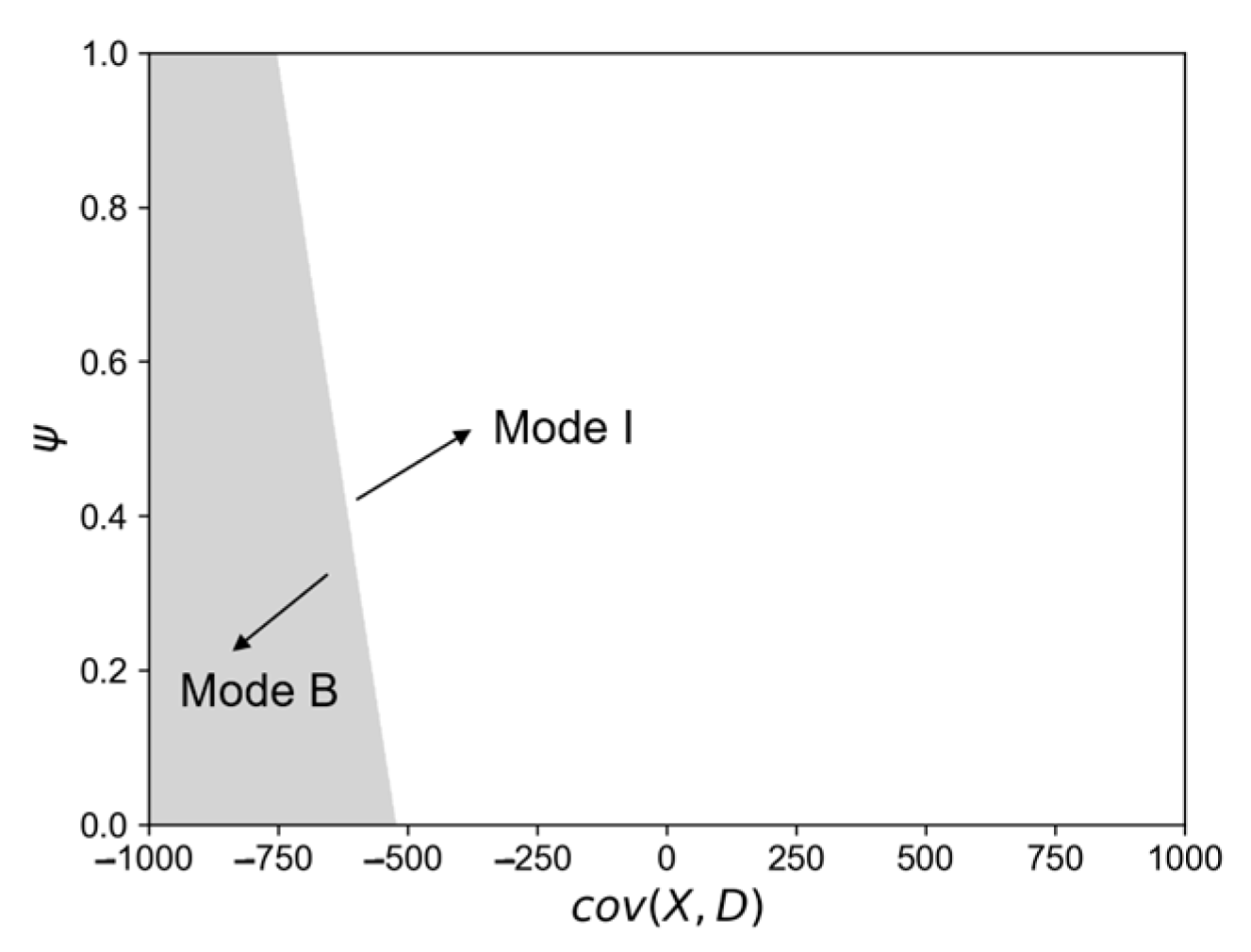
The correlation between exchange rate and demand affects supplier profit and, subsequently, the logistics mode choice. When the correlation is high, exchange rate fluctuations can quickly influence demand, resulting in the instability of demand. At this time, suppliers may prefer mode I to respond directly to demand changes and seize sales opportunities quickly. When the correlation is low, it indicates that market demand is less sensitive to exchange rate fluctuations and that consumer purchasing behavior is more stable. At this time, adopting mode B can provide full play to the advantages of logistics costs, improving logistics efficiency through centralized inventory management and batch order processing, providing more stable supply chain management.

6.2. Managerial Implications

Based on the research conclusions of this paper, we derive the following four managerial implications:

(i)

Suppliers should consider product profit margins and market risk to optimize their product portfolios. For high-profit products, increase inventory during periods of high demand volatility to ensure customer demand is met during market peaks, thus seizing profit opportunities. Conversely, inventory should be reduced during high exchange rate volatility to avoid profit losses caused by exchange rate fluctuations. For low-profit products, adopt the opposite strategy. This approach maintains profits while reducing the risk associated with market uncertainties. In addition, suppliers should closely monitor market demand changes and dynamically adjust the amount of stock in overseas warehouses to reduce inventory risk. Different inventory strategies should be adopted to respond to exchange rate changes. Increase inventory during currency depreciation to capitalize on export benefits and reduce export inventory during currency appreciation.

(ii)

Choosing an appropriate logistics mode to respond to changes in market demand. When the level of market demand is low and market fluctuations are high, suppliers should adopt mode I to improve the flexibility of response to the market. Mode I is suitable for quickly responding to small orders and testing new markets, reducing the risk of overinvestment and inventory backlog. When market demand is high, and market volatility is low, mode B should be prioritized to reduce unit logistics costs and improve operational efficiency through centralized storage and batch processing. This not only optimizes the cost structure but also strengthens market supply stability. To summarize, CBEC companies should regularly conduct market demand analysis, combine sales data with market trend forecasts, and adjust inventory and logistics deployment accordingly. Additionally, flexible logistics channels should be established to determine the appropriate logistics mode based on market demand, ensuring a balance between cost efficiency and market response speed.

(iii)

Selecting an appropriate logistics mode to cope with exchange rate fluctuations. When the logistics cost of overseas warehouses has apparent advantages, maintaining the overseas warehouse mode is a reasonable choice as it controls costs while ensuring supply chain efficiency. However, suppose the cost advantage of overseas warehousing decreases, for example, due to local policy changes, rising operating costs, etc. In that case, suppliers should re-evaluate the cost-effectiveness of both logistics modes and choose the most suitable one based on the extent of exchange rate appreciation or depreciation. When exchange rate volatility is low, a stable market environment allows for the use of the overseas warehouse mode to optimize costs and improve supply chain efficiency. Conversely, when exchange rate risk increases, suppliers should adopt mode I to mitigate risks with its inventory flexibility and quick market response capability. CBEC companies should enhance exchange rate forecasting and increase logistics flexibility, adjusting logistics strategies based on exchange rate trends.

(iv)

CBEC companies should consider the correlation between exchange rates and demand when choosing a logistics mode. Different logistics modes are selected according to the high or low correlation between exchange rate and demand in order to maximize market response speed, cost efficiency, and risk management. Mode I is suitable for markets with a high correlation between exchange rates and demand, allowing quick adaptation to environmental changes, such as in luxury goods. Mode B is more suitable for markets with relatively stable demand or less sensitive to exchange rate fluctuations, such as necessities. The correlation between exchange rates and demand is closely related to product attributes and industries. Therefore, CBEC companies should conduct market analysis for different industries and product types, designing and implementing efficient logistics solutions for different product categories.

6.3. Future Research Directions

There are still many exciting and worthwhile areas for future research. First, this paper considers a supply chain structure consisting of a supplier and an e-commerce platform, exploring the supplier’s logistics mode choice under demand and exchange rate risks. Future research could consider logistics mode choices under different CBEC supply chain structures. Second, this paper focuses on the supplier’s inventory strategy and logistics mode choice under exchange rate risks and analyzes the impact of demand and exchange rate uncertainties. However, it does not consider the management of exchange rate risks. Therefore, financial hedging and risk-sharing for exchange rate risks in CBEC are also topics worth exploring.

References

- Niu, B.Z.; Chen, K.L.; Chen, L.; Ding, C.; Yue, X.H. Strategic waiting for disruption forecasts in cross-border e-commerce operations. Prod. Oper. Manag. 2021, 30, 2840–2857. [Google Scholar] [CrossRef]
- Li, X.F.; Ma, J.; Li, S. Intelligence customs declaration for cross-border e-commerce based on the multi-modal model and the optimal window mechanism. Ann. Oper. Res. 2022, 1–25. [Google Scholar] [CrossRef] [PubMed]
- Zhang, X.M.; Zha, X.Y.; Dan, B.; Liu, Y.; Sui, R.H. Logistics mode selection and information sharing in a cross-border e-commerce supply chain with competition. Eur. J. Oper. Res. 2024, 314, 136–151. [Google Scholar] [CrossRef]
- Belt and Road Portal. China’s Cross-Border e-Commerce Imports and Exports Total 2.38 Trillion Yuan in 2023, up 15.6 Percent. Available online: https://www.yidaiyilu.gov.cn/p/0JPOMQMJ.html (accessed on 15 June 2024).
- Global e-Commerce Sales Reach $6.3 Trillion by 2023. Available online: https://www.ennews.com/news-65332.html (accessed on 15 June 2024).
- Wang, M.; Zhao, L.D.; Herty, M. Logistics service sharing of sellers on an e-commerce platform considering the behavior of carbon emission pooling. Electron. Commer. Res. Appl. 2023, 59, 101267. [Google Scholar] [CrossRef]
- Amazon. Standard Selling Expenses. Available online: https://sell.amazon.com/zh/pricing (accessed on 15 June 2024).
- Does Tmall Global Require a Commission for Opening a Store? Can Individuals Open a Store? Available online: https://www.xeeger.com/article/23726 (accessed on 15 June 2024).
- Zha, X.Y.; Zhang, X.M.; Liu, Y.; Dan, B. Bonded-warehouse or direct-mail? Logistics mode choice in a cross-border e-commerce supply chain with platform information sharing. Electron. Commer. Res. Appl. 2022, 54, 101181. [Google Scholar] [CrossRef]
- Niu, B.Z.; Ruan, Y.Y. Self-reliant shipping to mitigate disruption risk in the direct-delivery channel: Will the e-tailer’s bonded-warehouse channel also benefit? Marit. Policy Manag. 2023, 1–28. [Google Scholar] [CrossRef]
- Song, B.; Yan, W.; Zhang, T.J. Cross-border e-commerce commodity risk assessment using text mining and fuzzy rule-based reasoning. Adv. Eng. Inform. 2019, 40, 69–80. [Google Scholar] [CrossRef]
- Shao, B.J.; Cheng, Z.D.; Wan, L.J.; Yue, J. The impact of cross border E-tailer’s return policy on consumer’s purchase intention. J. Retail. Consum. Serv. 2021, 59, 102367. [Google Scholar] [CrossRef]
- Shi, X.; Wang, H. Design of the cost allocation rule for joint replenishment to an overseas warehouse with a piecewise linear holding cost rate. Oper. Res. Int. J. 2022, 22, 4905–4929. [Google Scholar] [CrossRef]
- Hazarika, B.B.; Mousavi, R. Review of Cross-Border E-Commerce and Directions for Future Research. J. Glob. Inf. Manag. 2022, 30, 1–18. [Google Scholar] [CrossRef]
- Chen, X.; Li, B.; Song, D.P.; Wang, M.X. Influences of risk-aversion behavior and purchasing option in a cross-border dual-channel supply chain. Int. Trans. Oper. Res. 2023, 1–30. [Google Scholar] [CrossRef]
- The 2022 “Cross-border E-commerce Financial Services Report”. Available online: https://www.ebrun.com/report/512935.shtml (accessed on 15 June 2024).
- Zhiou Technology IPO: Relies on Overseas e-Commerce Amazon, Exchange Loss Exceeds 70 Million with Capital Risk. Available online: https://m.thepaper.cn/baijiahao_20576220 (accessed on 15 June 2024).
- US Dollar Index Edges Lower, Yen Expected to Appreciate Significantly—2024 Global Forex Market Outlook. Available online: https://www.163.com/dy/article/IP7U82Q805199DKK.html (accessed on 15 June 2024).
- Wang, X.; Xie, J.; Fan, Z.P. B2C cross-border E-commerce logistics mode selection considering product returns. Int. J. Prod. Res. 2021, 59, 3841–3860. [Google Scholar] [CrossRef]
- Niu, B.Z.; Chen, L.Y.; Wang, J.M. Ad valorem tariff vs. specific tariff: Quality-differentiated e-tailers’ profitability and social welfare in cross-border e-commerce. Omega 2022, 108, 102584. [Google Scholar] [CrossRef]
- Zhang, M.D.; Pratap, S.; Zhao, Z.H.; Prajapati, D.; Huang, G.Q. Forward and reverse logistics vehicle routing problems with time horizons in B2C e-commerce logistics. Int. J. Prod. Res. 2021, 59, 6291–6310. [Google Scholar] [CrossRef]
- Xie, F.J.; Feng, R.C.; Zhou, X.Y. Research on the optimization of cross-border logistics paths of the “belt and road” in the inland regions. J. Adv. Transport. 2022, 2022, 5776334. [Google Scholar] [CrossRef]
- Liu, X.; Zhang, K.; Chen, B.; Zhou, J.; Miao, L. Analysis of logistics service supply chain for the One Belt and One Road initiative of China. Transport. Res. E Log. 2018, 117, 23–39. [Google Scholar] [CrossRef]
- Ren, S.; Choi, T.M.; Lee, K.M.; Lin, L. Intelligent service capacity allocation for cross-border-E-commerce related third-party-forwarding logistics operations: A deep learning approach. Transport. Res. E Log. 2020, 134, 101834. [Google Scholar] [CrossRef]
- Han, S.H.; Chen, S.; Yang, K.; Li, H.C.; Yang, F.J.; Luo, Z.W. Free shipping policy for imported cross-border e-commerce platforms. Ann. Oper. Res. 2024, 335, 1537–1566. [Google Scholar] [CrossRef]
- Giuffrida, M.; Mangiaracina, R.; Perego, A.; Tumino, A. Cross-border B2C e-commerce to China: An evaluation of different logistics solutions under uncertainty. Int. J. Phys. Distrib. Log. Manag. 2020, 50, 355–378. [Google Scholar] [CrossRef]
- Kim, K.K.; Park, K.S. Transferring and sharing exchange-rate risk in a risk-averse supply chain of a multinational firm. Eur. J. Oper. Res. 2014, 237, 634–648. [Google Scholar] [CrossRef]
- Ogunranti, G.A.; Ceryan, O.; Banerjee, A. Buyer-supplier currency exchange rate flexibility contracts in global supply chains. Eur. J. Oper. Res. 2021, 288, 420–435. [Google Scholar] [CrossRef]
- Kazaz, B.; Dada, M.; Moskowitz, H. Global Production Planning Under Exchange-Rate Uncertainty. Manag. Sci. 2005, 51, 1101–1119. [Google Scholar] [CrossRef]
- Park, J.H.; Kazaz, B.; Webster, S. Risk mitigation of production hedging. Prod. Oper. Manag. 2017, 26, 1299–1314. [Google Scholar] [CrossRef]
- Gheibi, S.; Kazaz, B.; Webster, S. Capacity reservation and sourcing under exchange-rate uncertainty. Decis. Sci. 2021, 54, 257–276. [Google Scholar] [CrossRef]
- Li, S.L.; Wang, L.T. Outsourcing and capacity planning in an uncertain global environment. Eur. J. Oper. Res. 2010, 207, 131–141. [Google Scholar] [CrossRef]
- Liu, Z.G.; Nagurney, A. Supply chain outsourcing under exchange rate risk and competition. Omega 2011, 39, 539–549. [Google Scholar] [CrossRef]
- Hu, X.L.; Motwani, J.G. Minimizing downside risks for global sourcing under price-sensitive sensitive stochastic demand, exchange rate uncertainties, and supplier capacity constraints. Int. J. Prod. Econ. 2014, 147, 398–409. [Google Scholar] [CrossRef]
- Park, J.; Kazaz, B.; Webster, S. Technical note-pricing below cost under exchange-rate risk. Prod. Oper. Manag. 2016, 25, 153–159. [Google Scholar] [CrossRef]
- Ding, Q.; Dong, L.X.; Kouvelis, P. On the integration of production and financial hedging decisions in global markets. Oper. Res. 2007, 55, 470–489. [Google Scholar] [CrossRef]
- Arcelus, F.J.; Gor, R.; Srinivasan, G. Foreign exchange transaction exposure in a newsvendor setting. Eur. J. Oper. Res. 2013, 227, 552–557. [Google Scholar] [CrossRef]
- Anson, J.; Boffa, M.; Matthias, H. Consumer arbitrage in cross-border e-commerce. Rev. Int. Econ. 2019, 27, 1234–1251. [Google Scholar] [CrossRef]
- Gabrel, V.; Murat, C.; Thiele, A. Recent advances in robust optimization: An overview. Eur. J. Oper. Res. 2014, 235, 471–483. [Google Scholar] [CrossRef]
- Scarf, H. A min-max solution to an inventory problem. In Studies in the Mathematical Theory of Inventory and Production; Stanford University Press: Stanford, CA, USA; California, CA, USA, 1958; pp. 201–209. Available online: https://www.cambridge.org/core/journals/mathematical-gazette/article/abs/studies-in-the-mathematical-theory-of-inventory-and-production-by-k-j-arrow-s-karlin-and-h-scarf-pp-x-340-70s-1958-stanford-university-press-oup-london/1E93D92940792E412A9586692E541ADF (accessed on 15 June 2024).
- Gallego, G.; Moon, I. The distribution free newsboy problem: Review and extensions. J. Oper. Res. Soc. 1993, 44, 825–834. [Google Scholar] [CrossRef]
- Moon, I.; Gallego, G. Distribution free procedures for some inventory models. J. Oper. Res. Soc. 1994, 45, 651–658. [Google Scholar] [CrossRef]
- Ben-Tal, A.; Golany, B.; Nemirovski, A.; Vial, J.P. Retailer-supplier flexible commitments contracts: A robust optimization approach. Manuf. Serv. Oper. Manag. 2005, 7, 248–271. [Google Scholar] [CrossRef]
- Qiu, R.Z.; Shang, J. Robust optimization for risk-averse multi-period inventory decision with partial demand distribution information. Int. J. Prod. Res. 2014, 52, 7472–7495. [Google Scholar] [CrossRef]
- Murray, C.C.; Gosavi, A.; Talukdar, D. The multi-product price-setting newsvendor with resource capacity constraints. Int. J. Prod. Econ. 2012, 138, 148–158. [Google Scholar] [CrossRef]
- Zhang, J.; Xie, W.; Sarin, S.C. Robust multi-product newsvendor model with uncertain demand and substitution. Eur. J. Oper. Res. 2021, 293, 190–202. [Google Scholar] [CrossRef]
- Wang, Y.; Xiao, L.; Luo, X.G. On the optimal solution of a distributionally robust multi-product newsvendor problem. J. Oper. Res. Soc. 2022, 74, 2578–2592. [Google Scholar] [CrossRef]
- Chen, L.; He, S.M.; Zhang, S.Z. Tight Bounds for Some Risk Measures, with Applications to Robust Portfolio Selection. Oper. Res. 2011, 59, 847–865. [Google Scholar] [CrossRef]
- Yu, H.; Yan, X.L. Advance selling under uncertain supply and demand: A robust newsvendor perspective. Int. Trans. Oper. Res. 2022, 31, 2672–2715. [Google Scholar] [CrossRef]
- Bai, Q.G.; Xu, J.T.; Gong, Y.M.; Satyaveer, S.C. Robust decisions for regulated sustainable manufacturing with partial demand information: Mandatory emission capacity versus emission tax. Eur. J. Oper. Res. 2022, 298, 874–893. [Google Scholar] [CrossRef]
- Koçyiğit, C.; Iyengar, G.; Kuhn, D.; Wiesemann, W. Distributionally robust mechanism design. Manag. Sci. 2020, 66, 159–189. [Google Scholar] [CrossRef]
- Chen, L.; Dong, T.; Peng, J.; Ralescu, D. Uncertainty analysis and optimization modeling with application to supply chain management: A systematic review. Mathematics 2023, 11, 2530. [Google Scholar] [CrossRef]
- Fu, Q.; Sim, C.K.; Teo, C.P. Profit sharing agreements in decentralized supply chains: A distributionally robust approach. Oper. Res. 2018, 66, 500–513. [Google Scholar] [CrossRef]
- Zhong, Y.G.; Liu, J.; Zhou, Y.W.; Cao, B.; Cheng, T.C.E. Robust contract design and coordination under consignment contracts with revenue sharing. Int. J. Prod. Econ. 2022, 253, 2672–2715. [Google Scholar] [CrossRef]
- Chen, Z.; Xie, W.J. Regret in the newsvendor model with demand and yield randomness. Prod. Oper. Manag. 2021, 30, 4176–4197. [Google Scholar] [CrossRef]
- Perakis, G.; Roels, G. Regret in the newsvendor model with partial information. Oper. Res. 2008, 56, 188–203. [Google Scholar] [CrossRef]
- Ha, A.Y.; Luo, H.; Shang, W. Supplier encroachment, information sharing, and channel structure in online retail platforms. Prod. Oper. Manag. 2021, 31, 1235–1251. [Google Scholar] [CrossRef]
- What Are the Charging Standards of AliExpress? An Introduction to the Cost Composition and Calculation Method! Available online: https://www.amzdh.com/smtwem/4634.html (accessed on 15 June 2024).
- Gao, F.; Su, X. Omnichannel retail operations with buy-online-and-pick-up-in-store. Manag. Sci. 2017, 63, 2478–2492. [Google Scholar] [CrossRef]
- Jiang, L.; Anupindi, R. Customer-driven vs. retailer-driven search: Channel performance and implications. Manuf. Serv. Oper. Manag. 2010, 12, 102–119. [Google Scholar] [CrossRef]
- Lee, C.M.; Hsu, S.L. The effect of advertising on the distribution-free newsboy problem. Int. J. Prod. Econ. 2011, 129, 217–224. [Google Scholar] [CrossRef]
- The Japanese Yen Exchange Rate Plummets! The Lowest Price in 34 Years Boosts Luxury Goods Sales! Available online: https://baijiahao.baidu.com/s?id=1797588656965601257&wfr=spider&for=pc (accessed on 15 June 2024).