Dynamic Pricing and Commission Strategies in Live-Stream: An Incentive Mechanism Analysis

Abstract

This paper explores optimal strategies for manufacturers, streamers, and retailers in a dual-channel environment, focusing on three commission structures and two power structures. Our analysis identifies steady states where dynamic commissions converge, enhancing profitability and stability for all parties. We find that less dominant partners prefer commission structures that reinforce existing power structures. Profitability is influenced by dynamic commissions: under manufacturer dominance, dynamic wholesale price and commission rate increase profitability for manufacturers and retailers while decreasing streamers’ profits. In contrast, under streamer dominance, a dynamic commission rate enhances streamers’ profits but reduces those of manufacturers and retailers. This evaluation highlights the shared interests between manufacturers and retailers. Taking the spillover effect into account, commission strategies should consider hassle cost, initial commission rate, and spillover impact. Product selection strategies show consistent trends, with moderate hassle cost and a disutility factor ranging from moderate to high, regardless of the spillover effect.

1. Introduction

Live-stream e-commerce has revolutionized the retail industry, as streamers leverage their social media presence to create engaging shopping experiences that surpass traditional retail. By using their unique personalities and interactive techniques, streamers effectively promote brands and drive sales [1,2,3], playing a crucial role in the industry. However, the varying influences of streamers present challenges for revenue optimization, complicating the prediction and enhancement of financial returns. The current literature lacks sufficient exploration into how dynamic pricing and commission rate structures, influenced by streamer characteristics and power dynamics, can effectively address these challenges. Our study fills this gap by explicitly investigating manufacturers’ strategic decisions when partnering with High-influence (H) and Low-influence (L) streamers [4] under two distinct scenarios: “streamer-dominating”, where emerging brands leverage H-streamers to boost market visibility, and “manufacturer-dominating”, involving established brands using L-streamers.

Dynamic pricing plays a vital role in sectors like agriculture and manufacturing, where market forces significantly influence prices [5]. For instance, fluctuations in agricultural product prices, such as pork and eggs, and variations in dealer performance in the automotive industry illustrate the importance of flexible pricing. The Ministry of Agriculture and Rural Affairs closely tracks these fluctuations, highlighting the need for flexible wholesale pricing [6]. Manufacturers who adjust wholesale prices based on sales volume not only increase market share and profitability but also motivate dealers to improve sales, making this strategy essential for managing market volatility and optimizing supply chain efficiency [7].

The commission structure is critical for the financial success of partnerships. Traditional commission structures struggle to adapt to market volatility, causing disputes and inefficiencies. Many companies invest heavily in live-stream events with streamers, yet fixed high commission rates fail to incentivize active promotion, resulting in poor sales performance [8]. This lack of motivation for streamers highlights the shortcomings of current commission structures. Additionally, a search on the China Judgment Document Network reveals numerous contract disputes related to “live-stream promotion”, many involving MCN agencies that failed to meet sales targets [9]. To address these issues, our research proposes dynamic commission structures that adjust with sales performance. By linking commission rates directly to sales data, our model aligns incentives, fosters sustainable collaboration, and optimizes profits.

We introduce dynamic commission structures involving wholesale prices and commission rates, integrating sales data across periods to guide decision-making. These structures enable all parties to optimize short- and long-term profits while encouraging sustainable collaboration. Similar dynamic commission schemes, employed by companies like HubSpot and Salesforce, incentivize sales representatives to prioritize lasting customer relationships over single transactions.

This study explores dual-channel distribution across six scenarios, combining three commission structures with two power structures: manufacturer-dominating (EM, DWM, DDW) and streamer-dominating (ES, DWS, DDS). We examine how variations in dynamic wholesale price and commission rate influence profitability within these scenarios. Specifically, we address the following questions: (i) How do variables change under dynamic commission structures, and do cooperative states stabilize or fluctuate? How do these dynamics shift across power structures? (ii) What are the partnership preferences for manufacturers, streamers, and retailers under various commission structures? (iii) Which commission structure is optimal for each party, and what factors influence these choices? (iv) Can a distribution strategy satisfy the margins of all three parties under a given commission structure? and (v) How do strategic choices change with the spillover effect, and what drives these changes?

To address these questions, we developed a game-theoretic dual-channel distribution model that reflects the interactions between manufacturers, streamers, and retailers. The model incorporates three commission structures within two power structures, enabling a comprehensive analysis of how dynamic commission rates and dynamic wholesale price influence profitability and strategy.

We introduced a dynamic wholesale price adjustment mechanism to examine its impact on profitability across various product types and parameter settings. By incorporating spillover effects, we also assessed how externalities shape strategic decisions and profit distributions. The model’s robustness was tested through sensitivity analysis, providing insights into the effects of key parameter changes on cooperation stability, profit distribution, and strategic decisions. This methodological framework allowed us to derive actionable recommendations and enhance the model’s practical relevance.

This study contributes to the live-stream literature in five ways. First, it demonstrates that dynamic commission structures can significantly enhance profitability for manufacturers, streamers, and retailers, providing practical solutions for stabilizing cooperation in volatile supply chains. Second, it offers strategic guidance for selecting partners and commission structures, helping stakeholders refine their approaches to improve profitability under dynamic market conditions. Third, the analysis identifies optimal product distribution types and initial commission rate ranges, offering clear recommendations for maximizing joint profits and aligning incentives. Fourth, the inclusion of spillover effects provides a more realistic perspective, revealing how external factors influence strategic decisions, thereby enhancing the relevance of dual-channel retail research. Finally, our examination of dynamic pricing mechanisms and their interaction with market power structures provides new theoretical insights into strategic dynamics, highlighting how manufacturers, streamers, and retailers can adjust their strategies depending on the prevailing power structure.

The remainder of this paper is organized as follows: Section 2 reviews related literature, Section 3 introduces six models based on dynamic commissions, Section 4 presents extended models considering spillover effect, Section 5 conducts numerical studies, and Section 6 concludes the study. All proofs are provided in the Appendix.

2. Literature Review

This study explores live-stream commerce, streamer type and power structure, and dynamic commissions, topics that will be reviewed in the following sections.

2.1. Live-Stream Commerce

Since the rise of live-stream commerce in 2016, academic research has increasingly focused on empirical studies [1,10,11,12]. Wongkitrungrueng and Assarut (2020) [1] found that live-stream is effective in increasing sales, enhancing consumer experience, and building engagement. Kang et al. (2021) [13] show that proper interactivity can drive consumers’ engagement on live-stream platforms. Based on the conclusions of [1,3,13], we incorporate the concept that live-stream brings extra value to consumers into our model setting. With its growing popularity, many researchers have based their studies on channel modeling [14,15,16,17]. The literature primarily focuses on pricing strategies [3,18,19], sales format selection [20,21], selling modes [22,23,24,25], capacity decisions [26], and quality decisions [4]. Analytical studies such as those by [27,28] employ game theory to explore the strategic interactions between unions/streamers and platforms, identifying optimal decision-making frameworks. Wang and Zhang (2023) [21] investigate the conditions under which manufacturers should adopt live-stream channels, concluding that while beneficial, adoption depends on factors like potential misfit elimination and consumer hassle costs. Contrasting views on the impact of live-stream on sales formats and pricing strategies are presented by [19,20], with the latter emphasizing the retailer’s willingness to adopt agency selling when live-stream is involved. Pan et al. (2022) [3] and Liu et al. (2024) [29] explore the impact of live-stream on traditional sales channels and consumer behavior, highlighting the importance of streamers’ selling ability and consumer factors such as anticipated regret and search costs. These studies collectively provide a foundation for understanding the strategic implications of live-stream selling. Building on these motivations, our research develops a model that captures essential features of both traditional online and live-stream channels. Despite this growing body of work, there is a gap in the literature regarding the impact of commission structures and power structures on manufacturers’ decisions within the live-stream context. This study aims to bridge this gap by focusing on how sales volume influences commission structures in both traditional online and live-stream sales and by investigating the decision-making dynamics between manufacturers and streamers under different power structures.

2.2. Streamer Type and Power Structure

Our research builds on the growing literature examining streamer types in live-stream e-commerce. Huang et al. (2021) [22] distinguish between celebrity and corporate streamers to guide the streamer selection strategy of manufacturers by empirically exploring the interaction effects between streamer type and product type on consumers’ purchase intentions and behavior in live-stream. While Hou et al. (2021) [18] model streamer characteristics to determine the pricing policy for manufacturers. They distinguish between the two types of streamers by the value of social influence and discover that a larger social influence is always preferred by manufacturers when selecting a streamer. Qi et al. (2022) [26] study streamer characteristics and bargaining power for effective live-stream strategies. They distinguish between two types of streamers by the form of commission, in which the regular streamer has less bargaining power and charges a per-unit commission. However, with more bargaining power, the top streamer can demand a fixed payment besides a per-unit commission. Their finding reveals that manufacturers should not necessarily prioritize top streamers with high bargaining power. This contrasts with [18], who argue that larger social influence is always preferred. Based on [24,26] classify streamer types using their popularity, negotiating power, and commission payment methods and analyze seller preferences for different types of streamers and associated pricing strategies. Niu et al. (2024) [23] analyze whether to start live-stream selling and which live-stream selling strategy to adopt between the self-live-stream strategy and the top streamer-live-stream strategy, considering the nature of streamers and cooperation methods with manufacturers. Similarly, Zhang et al. (2023b) [25] categorize streamers based on their nature and ways of cooperation with manufacturers. Zhang et al. (2023) [4] analyze the impact of top streamers and ordinary streamers on the quality decision of live-stream e-commerce supply chains. These studies highlight the importance of classifying streamers according to their characteristics and their collaboration model with manufacturers, which directly influences the manufacturers’ channel and pricing strategies.

Similar to the research by [24,26], our study proposes that different streamer types wield varying bargaining power. Differently, we examine how the streamer type influences strategic decisions on commission structures. In addition, our practical observations reveal that in certain live-stream showrooms, some streamers present products over several days, potentially due to uncertainties in fulfilling negotiated commitments with merchants. In such cases, H-streamers may require a commitment to specific quantities, which they ultimately must fulfill. Reflecting this practical context, our model incorporates a variable decision subject related to sales volume when collaborating with H-streamers. Our study thus integrates a dynamic perspective on decision-making, emphasizing the importance of power structure within the live-stream sales context.

Huang et al. (2016) [30] examine how different power structures affect supply chain performance. Li et al. (2020) [31] analyze power dynamics in decentralized assembly systems. Hu et al. (2021) [32] examine strategic vertical integration decisions under distinct power structures. Zhang et al. (2023) [4] explore how the power characteristics of top and ordinary streamers influence quality decisions in live-stream e-commerce. These studies primarily reflect power dynamics by altering the game sequence, but our research proposes that power structures can also be represented by shifts in the key decision-makers (i.e., which party controls the decision variable), a factor often neglected in prior research.

Among the vast amounts of literature on manufacturers’ strategic decisions, Zhang et al. (2023b) [25] is the most relevant to our investigation of manufacturers’ optimal decisions regarding pricing strategies. Zhang et al. (2023b) [25] analyze manufacturers’ optimal decisions when choosing between merchant live-stream and external streamer live-stream formats, offering guidance on whether to use a live-stream channel. Our research builds on this by classifying external streamers into high-influence and low-influence categories and analyzing how power dynamics between the manufacturer and the streamers affect the optimal commission structures.

2.3. Dynamic Commission

Dynamic commission mechanisms introduce flexibility by linking commission rate to sales performance across multiple periods. This approach allows manufacturers to align streamers’ incentives more effectively, contrasting with traditional models that treat commission rates as static and exogenous [19,33,34,35,36,37,38,39,40,41]. While these static models provide foundational insights into commission structures, they fall short in addressing the dynamic nature of modern live-stream channels, where performance metrics often evolve across periods. Furthermore, conflicts between distribution channels amplify the significance of commission rates as a critical factor in shaping manufacturers’ strategic decisions on channel interactions.

Recent theoretical research has started exploring dynamic commission mechanisms [42,43,44,45,46,47,48]. For instance, Liu et al. (2020) [49] emphasize how market size influences the optimal commission rate. Tsunoda and Zennyo (2021) [48] explore a dynamic commission mechanism where the commission rate is adjusted based on a supplier’s choice between wholesale and agency models. The adjustment is influenced by external factors like market uncertainty, aiming to guide suppliers toward the sales model that maximizes the platform’s profit. Wei and Dong (2021) [44] investigate how retail platforms dynamically adjust the commission rate based on suppliers’ product differentiation and order fulfillment costs, aiming to optimize channel efficiency and competition between sales channels. These studies highlight the potential of a dynamic commission rate to improve channel efficiency and mitigate competition between sales channels.

While this body of research has laid important groundwork in understanding the endogenous adjustments of commission rate, it often emphasizes either exogenous factors such as market uncertainty or endogenous factors like product differentiation, leaving gaps in understanding how internal sales dynamics influence commission adjustments. Our research diverges by focusing on sales volume as a novel endogenous factor influencing commission rate. Specifically, we introduce a dynamic multi-period model that directly links commission rate to sales performance across periods. This approach moves beyond existing frameworks, which typically overlook the explicit connection between sales data and commission adjustments over a period.

Additionally, our research integrates concepts from the broader pricing literature [50,51,52,53,54,55], which examine how reference prices and consumer behavior influence strategic pricing decisions. By incorporating the reference price effect into the dynamic commission rate framework, we provide a more comprehensive model. This integration captures the evolving relationship between sales data and commission adjustments, offering insights into optimizing profits in a dynamic and performance-driven environment.

In conclusion, existing literature has extensively categorized streamers in live-stream e-commerce based on their influence and differentiated them by decision-making order or commission-sharing methods. However, it has largely overlooked the impact of distinct streamer types on manufacturers’ commission strategies within supply chain-dominant contexts. To bridge this gap, our study identifies two distinct types of streamers responsible for live channel sales decisions when manufacturers act as supply chain leaders. Furthermore, we explore how these different streamer types influence manufacturers’ strategies regarding commission structures. The unique contributions of our research are summarized in

Table 1. Differences between this study and prior studies.

Author	Year	Research Branch			Decision Variables	Exogenous	Endogenous		Single/Multi-Period	Multi-Period
		LC	ST/PS	DC			Y/N	Influential Factor		Y/N	$\mathbf{Period}\text{-}\mathbf{Varying} {\mathit{r}}_{\mathit{t}}$	$\mathbf{Period}\text{-}\mathbf{Varying} {\mathit{w}}_{\mathit{t}}$
Ji et al. [19]	2023	$\surd$	-	-	Retail Price	$\surd$	Y	BP	Single	N	N/A	N/A
Pan et al. [3]	2022	$\surd$	-	-	Retail Price	-	N	N/A	Single	N	N/A	N/A
Chen et al. [56]	2023a	-	$\surd$	-	Retail Price	N/A	N	N/A	Single	N	N/A	N/A
Wang and Zhang [21]	2023	$\surd$	-	$\surd$	Retail price	-	Y	MP, ME, SC, TC	Single	N	N/A	N/A
Tang et al. [57]	2023	-	$\surd$	$\surd$	Sales volume	$\surd$	Y	Selling cost	Single	N	N/A	N/A
Hu et al. [43]	2022	-	-	$\surd$	Retail price	-	Y	Marginal cost	Single	N	N/A	N/A
Sun et al. [58]	2020	-	-	-	Retail Price	N/A	N	N.A.	Multiple	Y	-	-
Chen et al. [59]	2019	-	-	-	Retail Price	N/A	N	N.A.	Multiple	Y	-	$\surd$
Liu et al. [29]	2024	$\surd$	-	-	Retail Price	-	N	N.A.	Single	N	N/A	N/A
Liu et al. [49]	2020	-	-	-	Sales volume	$\surd$	Y	Market size	Single	N	N/A	N/A
Chen et al. [60]	2024	$\surd$	-	-	Retail Price	-	N	N/A	Single	N	N/A	N/A
Niu et al. [23]	2024	$\surd$	$\surd$	-	Retail Price	$\surd$	N	N/A	Single	N	N/A	N/A
Hou et al. [18]	2021	$\surd$	$\surd$	-	Retail Price	$\surd$	N	N/A	Single	N	N/A	N/A
Yu et al. [61]	2022	$\surd$	$\surd$	-	Retail Price	$\surd$	N	N/A	Single	N	N/A	N/A
Zhang et al. [4]	2023	$\surd$	$\surd$	-	QIE, QTE	$\surd$	N	N/A	Single	N	N/A	N/A
Zhang et al. [25]	2023b	$\surd$	$\surd$	-	Retail Price	$\surd$	N	N.A.	Single	N	N/A	N/A
This paper	2024	$\surd$	$\surd$	$\surd$	Sales volume	$\surd$	$\surd$	Sales volume, commission	Multiple	Y	$\surd$	$\surd$

Note: $\surd$: considered, -: not considered, N/A: not applicable. LC: live-stream commerce. ST/PS: streamer type and power structure. DC: dynamic commission. BP: bargaining power. MP: misfit probability. ME: misfit elimination. SC: service cost. TC: travel cost. QIE: manufacturer’s quality improvement effort level. QTE: streamer’s quality testing effort level.

, highlighting how our approach contrasts with and extends the current body of literature.

3. Problem Description

In a supply chain offering products through both live-stream and traditional online channels, consumer experiences differ significantly, which affects purchase decisions. Studies show that live-stream provides a richer visual product experience compared to traditional online channels, which often lack detailed product descriptions [62]. However, live-stream may incur hassle costs, such as longer transaction time, potentially discouraging some consumers [3,16,21], denoted as $c_i$. Assuming consumers’ valuations are uniformly distributed between 0 and 1 and incorporating the disutility factor $\theta$ associated with the traditional online channel experience [63], we define consumers’ utility functions as $u_r=\theta v-p_r$ for traditional online channels and $u_l=v-p_l-c_i$ for live-stream channels, where $p_r$ and $p_l$ are retail prices in traditional online and live-stream channels.

In this dual-channel setting, consumers choose between live-stream and traditional online channels. Following [62,63], the marginal consumers, those who are between participating and not participating in the traditional online channel, are represented as ${\displaystyle \frac{p_r}{\theta }}.$ The type that is indifferent between both channels is denoted as ${\displaystyle \frac{p_l+c_i-p_r}{1-\theta }}$. Market segmentation is thus defined as $D_r={\displaystyle \frac{p_l\theta +c_i\theta -p_r}{\theta (1-\theta )}}$, $D_l={\displaystyle \frac{1-\theta -p_l-c_i+p_r}{1-\theta }}$, where $D_r$ and $D_l$ represent the sales volumes for traditional online and live-stream, respectively. Focusing on scenarios where the decision variable shifts from retail price to product supply quantity across channels [64], the inverse demand functions for the two channels are $p_r=\theta (1-D_l-D_r)$ and $p_l=1-D_l-D_r\theta -c_i$.

Table 2. Summary of notations.

Notations	Description
$b$	$\mathrm{Superscript} \mathrm{of} \mathrm{benchmark} \mathrm{models}, b\in \{EM,ES\}$
$k$	$\mathrm{Superscript} \mathrm{of} \mathrm{dynamic} \mathrm{models}, k\in \{DWM,DWS,DDM,DDS\}$.
$i$	$\mathrm{Superscript} \mathrm{of} \mathrm{manufacturer}\text{-}\mathrm{dominating} \mathrm{scenarios}, l\in \{EM,DWM,DDM\}$
$j$	$\mathrm{Superscript} \mathrm{of} \mathrm{streamer}\text{-}\mathrm{dominating} \mathrm{scenarios}, m\in \{ES,DWS,DDS\}$
$n$	Superscript of extended models
$M,S,R$	Subscript of manufacturer, streamer, and retailer
$r^h$$, r^l$	The commission rate paid by the manufacturer to the H- and L-streamers
$r$	$\mathrm{The} \mathrm{commission} \mathrm{rate} 0<r<1$.
$r_t$	$\mathrm{The} \mathrm{commission} \mathrm{rate} \mathrm{in} \mathrm{period} t$$, 0<r_t<1$.
${\pi }_{M,t}^{**}, {\pi }_{S,t}^{**}, {\pi }_{R,t}^{**}$	The profits of the manufacturer, streamer, and retailer under steady states
${\pi }_{M,t}, {\pi }_{S,t}, {\pi }_{R,t}$	$\mathrm{The} \mathrm{profits} \mathrm{of} \mathrm{the} \mathrm{manufacturer}, \mathrm{streamer}, \mathrm{and} \mathrm{retailer} \mathrm{in} \mathrm{period} t$
${\pi }_M^{SEMP},{\pi }_M^{SEMN}$	The profits under positive and negative spillover effects
Decision Variables	Description
$D_r$$, D_l$	The sales volume of the traditional online channel and the live-stream channel
$w$	The wholesale price
$D_{r,t}$$, D_{l,t}$	$\mathrm{The} t_{th}$ period sales volume of the traditional online channel and the live-stream channel
$w_t$	$\mathrm{The} t_{th}$ period wholesale price

summarizes the main notations.

The manufacturer adjusts the wholesale price and the commission rate to optimize sales performance in each channel. Detailed descriptions of these dynamic commissions are provided in the following section.

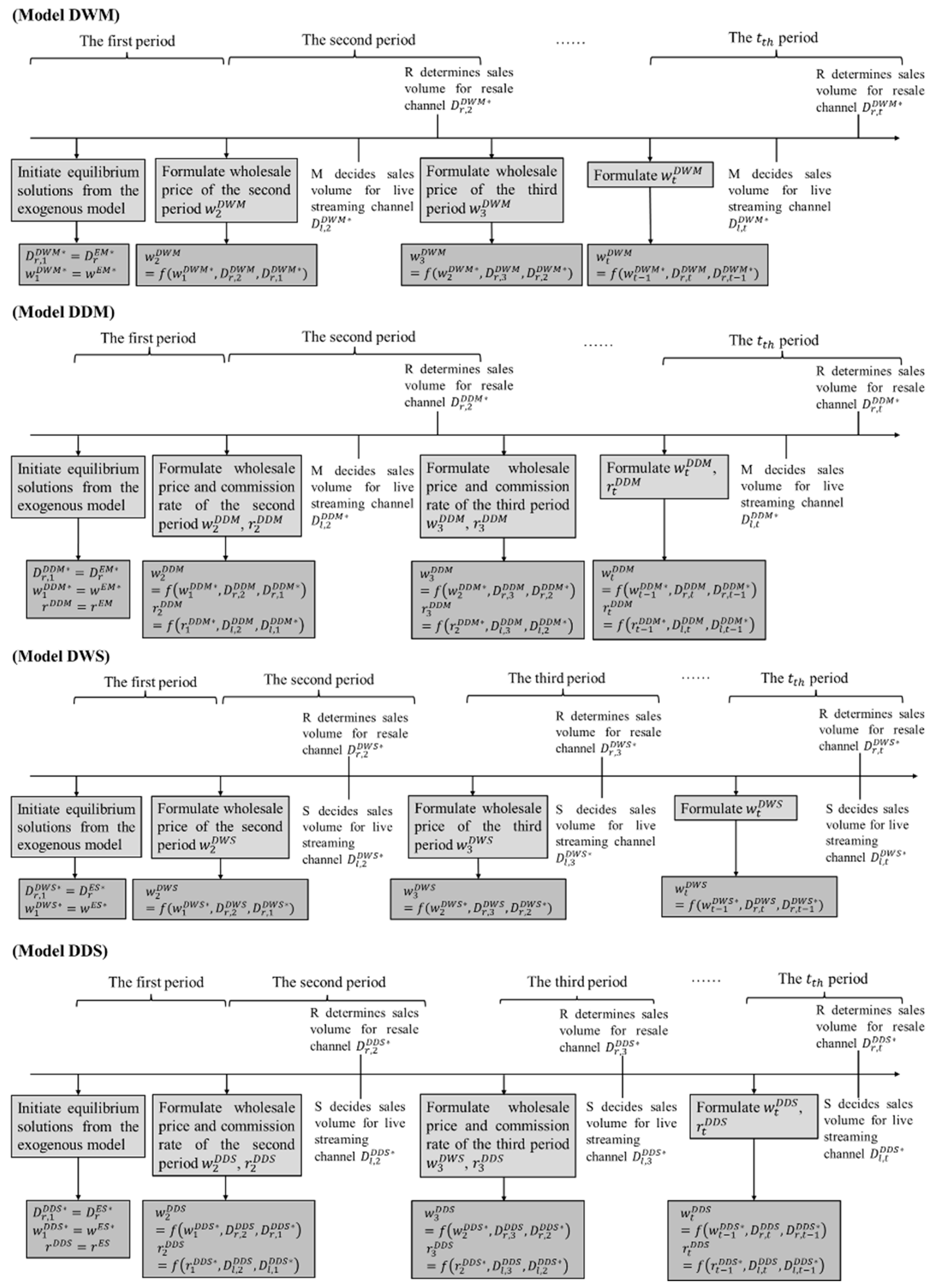
3.1. The Structure of Dynamic Wholesale Price and Commission Rate

Drawing upon the reference effect proposed by [50], we construct dynamic wholesale price and dynamic commission rate functions. According to economies of scale, the wholesale price is inversely related to sales volume. Building on this, we formulate the dynamic wholesale price as $w_t=\alpha g_{sv,t}+\left(1-\alpha \right)g_{wp,t}=\alpha \left[w_{t-1}\left(1-\left(D_{r,t}-D_{r,t-1}\right)\right)\right]+\left(1-\alpha \right)w_{t-1}$, where the memory parameter $\alpha \in \left(\mathrm{0,1}\right)$ indicates the dependence of the current wholesale price on past sales. The sale response factor $g_{sv,t}$ reflects the influence of consecutive sales performance on the current price, and the wholesale price response factor $g_{wp,t}$ shows the influence of the previous period’s wholesale price. A higher sales volume relative to the previous period, with a sales response factor below $w_{t-1}$, leads to a lower wholesale price, while lower sales result in a higher price. Similarly, the dynamic commission rate function is formulated as $r_t=\alpha f_{sv,t}+\left(1-\alpha \right)f_{cr,t}=\alpha \left[r_{t-1}\left(1+{\displaystyle \frac{D_{l,t}-D_{l,t-1}}{a{D}_{l,t}{D}_{l,t-1}}}\right)\right]+\left(1-\alpha \right)r_{t-1}$, with the constant $a$ ensuring the rate remains between 0 and 1 for each period $t=2,\dots T.$ The The manufacturer adjusts the commission rate $r_t$ based on the difference in live-stream channel sales $D_{l,t}-D_{l,t-1}$ and the previous period’s commission rate $r_{t-1}$. The sales response factor $f_{sv,t}$ signifies the effect of sales performance on the commission rate. The commission rate response factor $f_{cr,t}$ illustrates the influence of the prior period’s rate. If current sales exceed the previous period with a sales response factor above $r_{t-1}$, the commission rate increases. Otherwise, it decreases. Figure 1 depicts the sequence of the four dynamic models incorporating the two dynamic mechanisms.

3.2. Manufacturer-Dominating Scenarios

In manufacturer-dominating scenarios, the manufacturer, as the leader, first sets the sales volume $D_l^{EM*}$ for the live-stream channel and the wholesale price $w^{EM*}$ for the traditional online channel. The retailer then determines the sales volume $D_r^{EM*}$ for the traditional online channel. In Model DWM, the manufacturer replaces the fixed wholesale price with the dynamic function, and the Model DDM introduces dynamics for both the wholesale price and commission rate. Backward induction is used to determine optimal strategies [28,65]. When partnering with an L-streamer, the commission rate is $r^l=r^{EM}$ in Model EM, $r^l=r_1^{DWM}$ in Model DWM, and $r^l=r_1^{DDM}$ in Model DDM.

3.2.1. Model EM

Assuming that the manufacturer’s profit function ${\pi }_M^{EM}$ is jointly concave in $\left(D_l^{EM},w^{EM}\right)$, it guarantees the existence of a unique maximum. By applying first-order optimality conditions to the decision sequence, we derive equilibrium profits and decision variables.

Lemma 1.

In Model EM, for the manufacturer to maximize profits with a dual-channel strategy, the disutility factor and hassle cost must satisfy $2c_i+\theta -2<0$, and the commission rate must remain below $r_b^{EM}$.

A successful dual-channel sales strategy depends on maintaining a balance between hassle cost and consumer experience. If the traditional online channel consistently outperforms the live-stream channel, it may diminish the effectiveness of the dual-channel approach. Additionally, it is beneficial for the manufacturer to secure a significant profit share, particularly when the streamer’s commission rate is capped.

Lemma 2.

The optimal decision variables in Model EM, as well as the expected profits of the three parties, are summarized in

Table 3. Equilibrium outcomes in benchmark models.

Decision Variables	EM	ES
$w^{b*}$	${\displaystyle \frac{2\theta \left(r^{EM}-1\right)\left(\left(c_i+\frac{\theta }{2}-1\right)r^{EM}-\theta +2\right)}{{r^{EM}}^2\theta +\left(-4\theta +8\right)r^{EM}+4\theta -8}}$	${\displaystyle \frac{\left(4c_i{r}^{ES}-c_i\theta +2r^{ES}\theta -4r^{ES}-3\theta +8\right)\theta }{2\left(r^{ES}\theta -3\theta +8\right)}}$
$D_r^{b*}$	$-{\displaystyle \frac{\left(r^{EM}-1\right)\left(\left(c_i-1\right)r^{EM}-2c_i\right)}{{r^{EM}}^2\theta +\left(-4\theta +8\right)r^{EM}+4\theta -8}}$	${\displaystyle \frac{\left(-r^{ES}+2\right)c_i+r^{ES}}{8+\left(r^{ES}-3\right)\theta }}$
$D_l^{b*}$	${\displaystyle \frac{\left(-4c_i-\theta +4\right)r^{EM}+4c_i+2\theta -4}{{r^{EM}}^2\theta +\left(-4\theta +8\right)r^{EM}+4\theta -8}}$	${\displaystyle \frac{\left(c_i-3\right)\theta -8c_i+8}{16+\left(2r^{ES}-6\right)\theta }}$
${\pi }_M^{b*}$	$-{\displaystyle \frac{2\left(r^{EM}-1\right)\left(\left(c_i-1\right)\left(c_i+\frac{\theta }{2}-1\right)r^{EM}+\left(-c_i+\frac{1}{2}\right)\theta -{\left(c_i-1\right)}^2\right)}{{r^{EM}}^2\theta +\left(-4\theta +8\right)r^{EM}+4\theta -8}}$	${\displaystyle \frac{\begin{array}{c}\left({c_i}^2+\left(-4r^{ES}+6\right)c_i+4r^{ES}-3\right)\theta \\ -8{\left(c_i-1\right)}^2\left(-1+r^{ES}\right)\end{array}}{32+\left(4r^{ES}-12\right)\theta }}$
${\pi }_S^{b*}$	$-{\displaystyle \frac{\begin{array}{c}4\left(\left(\left(c_i-2\right)\theta -4c_i+4\right)r^{EM}-2\left(\theta -2\right)\left(c_i-1\right)\right)\\ r^{EM}\left(\left(c_i+\frac{\theta }{4}-1\right)r^{EM}-c_i-\frac{\theta }{2}+1\right)\end{array}}{{\left({r^{EM}}^2\theta +\left(-4\theta +8\right)r^{EM}+4\theta -8\right)}^2}}$	${\displaystyle \frac{{\left(\left(c_i-3\right)\theta -8c_i+8\right)}^2{r}^{ES}}{4{\left(8+\left(r^{ES}-3\right)\theta \right)}^2}}$
${\pi }_R^{b*}$	${\displaystyle \frac{\theta {\left(r^{EM}-1\right)}^2{\left(\left(c_i-1\right)r^{EM}-2c_i\right)}^2}{{\left({r^{EM}}^2\theta +\left(-4\theta +8\right)r^{EM}+4\theta -8\right)}^2}}$	${\displaystyle \frac{{\theta \left(\left(c_i-1\right)r^{ES}-2c_i\right)}^2}{{\left(8+\left(r^{ES}-3\right)\theta \right)}^2}}$

.

Lemma 2 demonstrates the dynamics when a larger share of profits is allocated to the commission rate. As this rate increases, the manufacturer, despite its leading position, faces a growing disadvantage. In response, the manufacturer takes two strategic actions: first, reducing the live-stream channel’s sales volume by controlling product distribution (${\displaystyle \frac{\partial D_l^{EM*}}{\partial r^{EM}}}<0$); second, lowering the wholesale price for the retailer to encourage sales through the traditional online channel, thus enhancing profitability (${\displaystyle \frac{\partial w^{EM*}}{\partial r^{EM}}}<0$). These adjustments lead to both a decrease in the live-stream channel’s sales volume and a reduction in the wholesale price as the commission rate rises. The retailer responds by increasing sales in the traditional online channel, leveraging the lower wholesale cost (${\displaystyle \frac{{\partial D}_r^{EM*}}{\partial r^{EM}}}>0$). Consequently, the streamer benefits from the higher commission rate, resulting in increased profits. The retailer also profits by capitalizing the manufacturer’s adjustments to capture more sales through the traditional online channel. However, the manufacturer faces a challenge as its profits decline with the rising commission rate (${\displaystyle \frac{\partial {\pi }_S^{EM*}}{\partial r^{EM}}}>0$, ${\displaystyle \frac{\partial {\pi }_R^{EM*}}{\partial r^{EM}}}>0$, ${\displaystyle \frac{\partial {\pi }_M^{EM*}}{\partial r^{EM}}}<0$).

3.2.2. Model DWM

We initiate the solving process with the equilibrium solutions from the first period, $D_{r,1}^{DWM*}=D_r^{EM*}$ and $w_1^{DWM*}=w^{EM*}$. These data are used to calculate the second period’s wholesale price. The second-period wholesale price is then updated as: $w_2^{DWM}=\alpha \left[w_1^{DWM*}\left(1-\left(D_{r,2}^{DWM}-D_{r,1}^{DWM*}\right)\right)\right]+\left(1-\alpha \right)w_1^{DWM*}$. With this updated wholesale price, the retailer first determines the second-period sales volume $D_{r,2}^{DWM*}$ by maximizing their profit ${\pi }_{R,2}^{DWM}$, ${\pi }_{R,2}^{DWM}=\left(\theta \left(1-D_{l,2}^{DWM}-D_{r,2}^{DWM}\right)-w_2^{DWM}\right)D_{r,2}^{DWM}$. Next, the manufacturer optimizes the live-stream channel’s sales volume $D_{l,2}^{DWM*}$ to maximize their profit ${\pi }_{M,2}^{DWM}$, ${\pi }_{M,2}^{DWM}=w_2^{DWM}{D}_{r,2}^{DWM*}+\left(1-r^{DWM}\right)\left(1-D_{l,2}^{DWM}-D_{r,2}^{DWM*}\theta -c_i\right)D_{l,2}^{DWM}$. After determining the optimal decisions for the second period, $D_{l,2}^{DWM*}$, $D_{r,2}^{DWM*}$, $w_2^{DWM*}$, we proceed to the subsequent periods using the same method. This iterative process continues for each period $t^{\prime }$, producing a sequence of optimal decisions and corresponding profits. These include the optimal sales volumes for both channels, the wholesale price, the commission rate, and the profits for the manufacturer, streamer, and retailer: $\left\{D_{l,t^{\prime }}^{DWM*}\right\}$, $\left\{D_{r,t^{\prime }}^{DWM*}\right\}$, $\left\{w_{t^{\prime }}^{DWM*}\right\}$, $\left\{r_{t^{\prime }}^{DWM*}\right\}$, $\left\{{\pi }_{M,t^{\prime }}^{DWM*}\right\}$, $\left\{{\pi }_{S,t^{\prime }}^{DWM*}\right\}$, $\left\{{\pi }_{R,t^{\prime }}^{DWM*}\right\}$ where $t^{\prime }=\mathrm{1,2},\dots ,T-1,T$.

3.2.3. Model DDM

We start by setting the wholesale price and sales volumes for the first period as follows: $w_1^{DDM}=w^{EM}$, $r_1^{DDM}=r^{EM}$, $D_{l,1}^{DDM*}=D_l^{EM*}$, $D_{r,1}^{DDM*}=D_r^{EM*}$. For the second period, the commission rate $r_2^{DDM}$ and the wholesale price $w_2^{DDM}$ are updated: $r_2^{DDM}=\alpha \left[r_1^{DDM}\left(1+{\displaystyle \frac{D_{l,2}^{DDM}-D_{l,1}^{DDM*}}{a{D}_{l,2}^{DDM}{D}_{l,1}^{DDM*}}}\right)\right]+\left(1-\alpha \right)r_1^{DDM}=\alpha \left[r_1^{EM}\left(1+{\displaystyle \frac{D_{l,2}^{DDM}-D_{l,1}^{DDM*}}{a{D}_{l,2}^{DDM}{D}_{l,1}^{DDM*}}}\right)\right]+\left(1-\alpha \right)r_1^{EM}$, $w_2^{DDM}=\alpha \left[w_1^{DDM*}\left(1-\left(D_{r,2}^{DDM}-D_{r,1}^{DDM*}\right)\right)\right]+\left(1-\alpha \right)w_1^{DDM*}$. The retailer first determines the second-period sales volume $D_{r,2}^{DDM*}$ by maximizing their profit ${\pi }_{R,2}^{DDM}$, ${\pi }_{R,2}^{DDM}=\left(\theta \left(1-D_{l,2}^{DDM}-D_{r,2}^{DDM}\right)-w_2^{DDM}\right)D_{r,2}^{DDM}$. Next, the manufacturer optimizes the live-stream channel’s sales volume $D_{l,2}^{DDM*}$ to maximize their profit ${\pi }_{M,2}^{DDM}$, ${\pi }_{M,2}^{DDM}=w_2^{DDM}{D}_{r,2}^{DDM}+\left(1-r^{DDM}\right)\left(1-D_{l,2}^{DDM}-D_{r,2}^{DDM}\theta -c_i\right)D_{l,2}^{DDM}$. We then derive the optimal decision variables for the second period: $r_2^{DDM*}, D_{l,2}^{DDM*}$, $w_2^{DDM*}, D_{r,2}^{DDM*}$. This approach is repeated for all subsequent periods. After each period’s calculation, we establish a trajectory for all variables and profits: $\left\{D_{l,t^{\prime }}^{DDM*}\right\}$, $\left\{D_{r,t^{\prime }}^{DDM*}\right\}$, $\left\{w_{t^{\prime }}^{DDM*}\right\}$, $\left\{r_{t^{\prime }}^{DDM*}\right\}$, $\left\{{\pi }_{M,t^{\prime }}^{DDM*}\right\}$, $\left\{{\pi }_{S,t^{\prime }}^{DDM*}\right\}$, $\left\{{\pi }_{R,t^{\prime }}^{DDM*}\right\}$ where $t^{\prime }=\mathrm{1,2},\dots ,T-1,T$.

3.3. Streamer-Dominating Scenarios

In streamer-dominating scenarios, the streamer has significant influence, and decision-making in the live-stream channel transitions from the manufacturer to the streamer, forming a two-stage sequential game. First, the manufacturer sets the wholesale price $w^{ES*}$. Next, the streamer and retailer simultaneously determine their respective sales volumes, $D_l^{ES*}$ and $D_r^{ES*}$. In Model DWS, the manufacturer sets a fixed commission rate $r^{DWS}$ and implements a dynamic wholesale price function $w_t^{DWS}$. In Model DDS, both the commission rate $r_t^{DDS}$ and wholesale price $w_t^{DDS}$ are dynamic. When partnering with an H-streamer, the commission rate is $r^h=r^{ES}$ in Model ES, $r^h=r_1^{DWS}$ in Model DWS, $r^h=r_1^{DDS}$ in Model DDS. Equilibrium outcomes of dynamic models are summarized in Appendix A 

Table A1. The equilibrium results of dynamic models.

Decision Variables	$\mathbf{The} \mathbf{Equilibrium} \mathbf{Results} \mathbf{for} \mathbf{Each} \mathbf{Period} \mathit{t}$
$D_{r,t}^{DWM*}$	${\displaystyle \frac{\begin{array}{c}\left(1-r^{DWM}\right){\theta }^3+\left(\left(D_{r,t-1}^{DWM*}\alpha +1\right)\left(r^{DWM}-2\right)w_{t-1}^{DWM*}+2\left(r^{DWM}-1\right)\left(c_i+1\right)\right){\theta }^2-2w_{t-1}^{DWM*}\left(r^{DWM}-1\right)\left(2+\left(c_i+2D_{r,t-1}^{DWM*}+1\right)\alpha \right)\theta +4\alpha {w_{t-1}^{DWM*}}^2\left(D_{r,t-1}^{DWM*}\alpha +1\right)\left(r^{DWM}-1\right)\end{array}}{\left(-4r^{DWM}+4\right){\theta }^3+\left(\left(4r^{DWM}-6\right)\alpha w_{t-1}^{DWM*}+8r^{DWM}-8\right){\theta }^2-16\alpha w_{t-1}^{DWM*}\left(r^{DWM}-1\right)\theta +8{\alpha }^2{w_{t-1}^{DWM*}}^2\left(r^{DWM}-1\right)}}$,
$D_{l,t}^{DWM*}$	${\displaystyle \frac{\begin{array}{c}\left(1-r^{DWM}\right){\theta }^3+\left(\left(\left(-2+\left(D_{r,t-1}^{DWM*}+1\right)r^{DWM}\right)\alpha +r^{DWM}\right)w_{t-1}^{DWM*}-2\left(r^{DWM}-1\right)\left(c_i-1\right)\right){\theta }^2+4w_{t-1}^{DWM*}\left(r^{DWM}-1\right)\alpha \left(\left(-\frac{\alpha D_{r,t-1}^{DWM*}}{4}-\frac{1}{4}\right)w_{t-1}^{DWM*}+c_i-1\right)\theta -2{\alpha }^2{w_{t-1}^{DWM*}}^2\left(r^{DWM}-1\right)\left(c_i-1\right)\end{array}}{\left(-2r^{DWM}+2\right){\theta }^3+\left(\alpha \left(2r^{DWM}-3\right)w_{t-1}^{DWM*}+4r^{DWM}-4\right){\theta }^2-8\alpha w_{t-1}^{DWM*}\left(r^{DWM}-1\right)\theta +4{\alpha }^2{w_{t-1}^{DWM*}}^2\left(r^{DWM}-1\right)}}$,
$w_t^{DWM*}$	${\displaystyle \frac{2\left(\begin{array}{c}\left(\frac{3w_{t-1}^{DWM*}\left(r^{DWM}-\frac{4}{3}\right)D_{r,t-1}^{DWM*}{\alpha }^2}{2}+\left(\left(\frac{3r^{DWM}}{2}-2\right)w_{t-1}^{DWM*}-\left(r^{DWM}-1\right)\left(c_i-4D_{r,t-1}^{DWM*}+1\right)\right)\alpha +4r^{DWM}-4\right){\theta }^2\\ -2\left(1+\left(D_{r,t-1}^{DWM*}-\frac{1}{4}\right)\alpha \right)\left(r^{DWM}-1\right){\theta }^3+\left(-6+\left(c_i-6D_{r,t-1}^{DWM*}+1\right)\alpha \right)\left(r^{DWM}-1\right)w_{t-1}^{DWM*}\alpha \theta +2{\alpha }^2{w_{t-1}^{DWM*}}^2\left(D_{r,t-1}^{DWM*}\alpha +1\right)\left(r^{DWM}-1\right)\end{array}\right)w_{t-1}^{DWM*}}{\left(-4r^{DWM}+4\right){\theta }^3+\left(\left(4r^{DWM}-6\right)\alpha w_{t-1}^{DWM*}+8r^{DWM}-8\right){\theta }^2-16\alpha w_{t-1}^{DWM*}\left(r^{DWM}-1\right)\theta +8{\alpha }^2{w_{t-1}^{DWM*}}^2\left(r^{DWM}-1\right)}},$
$D_{r,t}^{DWS*}$	${\displaystyle \frac{2\alpha w_{t-1}^{DWS*}{D}_{r,t-1}^{DWS*}-c_i\theta -\theta +2w_{t-1}^{DWS*}}{4\alpha w_{t-1}^{DWS*}+{\theta }^2-4\theta }}$,
$D_{l,t}^{DWS*}$	$-{\displaystyle \frac{D_{r,t-1}^{DWS*}\alpha \theta w_{t-1}^{DWS*}+2\alpha c_i{w}_{t-1}^{DWS*}-2\alpha w_{t-1}^{DWS*}-2c_i\theta -{\theta }^2+\theta w_{t-1}^{DWS*}+2\theta }{4\alpha w_{t-1}^{DWS*}+{\theta }^2-4\theta }}$,
$w_t^{DWS*}$	${\displaystyle \frac{\left(\left(D_{r,t-1}^{DWS*}\alpha +1\right){\theta }^2+\left(-4+\left(c_i-4D_{r,t-1}^{DWS*}+1\right)\alpha \right)\theta +2\alpha w_{t-1}^{DWS*}\left(D_{r,t-1}^{DWS*}\alpha +1\right)\right)w_{t-1}^{DWS*}}{4\alpha w_{t-1}^{DWS*}+{\theta }^2-4\theta }}$,
$D_{r,t}^{DDM*}$	${\displaystyle \frac{\begin{array}{c}\left(r_{t-1}^{DDM*}\left(D_{l,t-1}^{DDM*}-1\right)\alpha -a{D}_{l,t-1}^{DDM*}\left(r_{t-1}^{DDM*}-1\right)\right){\theta }^3\\ +\left({\alpha }^2{r}_{t-1}^{DDM*}{w}_{t-1}^{DDM*}{D}_{r,t-1}^{DDM*}+\left(\left(D_{r,t-1}^{DDM*}a{r}_{t-1}^{DDM*}{w}_{t-1}^{DDM*}-2D_{r,t-1}^{DDM*}a{w}_{t-1}^{DDM*}-2r_{t-1}^{DDM*}\right)D_{l,t-1}^{DDM*}+2r_{t-1}^{DDM*}\left(c_i+\frac{w_{t-1}^{DDM*}}{2}+1\right)\right)\alpha +2a{D}_{l,t-1}^{DDM*}\left(r_{t-1}^{DDM*}\left(c_i+\frac{w_{t-1}^{DDM*}}{2}+1\right)-c_i-w_{t-1}^{DDM*}-1\right)\right){\theta }^2\\ -2\left(r_{t-1}^{DDM*}\left(c_i-D_{l,t-1}^{DDM*}+2D_{r,t-1}^{DDM*}+1\right){\alpha }^2+\left(a\left(r_{t-1}^{DDM*}-1\right)\left(c_i+2D_{r,t-1}^{DDM*}+1\right)D_{l,t-1}^{DDM*}+2r_{t-1}^{DDM*}\right)\alpha +2a{D}_{l,t-1}^{DDM*}\left(r_{t-1}^{DDM*}-1\right)\right)w_{t-1}^{DDM*}\theta +4\left(D_{r,t-1}^{DDM*}\alpha +1\right)\left(\alpha r_{t-1}^{DDM*}+a{D}_{l,t-1}^{DDM*}\left(r_{t-1}^{DDM*}-1\right)\right)\alpha {w_{t-1}^{DDM*}}^2\end{array}}{\begin{array}{c}\left(4{\alpha }^2{r}_{t-1}^{DDM*}{w}_{t-1}^{DDM*}+\left(4\left(r_{t-1}^{DDM*}-\frac{3}{2}\right)a{w}_{t-1}^{DDM*}{D}_{l,t-1}^{DDM*}+8r_{t-1}^{DDM*}\right)\alpha +8a{D}_{l,t-1}^{DDM*}\left(r_{t-1}^{DDM*}-1\right)\right){\theta }^2\\ \left(-4\alpha r_{t-1}^{DDM*}-4a{D}_{l,t-1}^{DDM*}\left(r_{t-1}^{DDM*}-1\right)\right){\theta }^3-16\left(\alpha r_{t-1}^{DDM*}+a{D}_{l,t-1}^{DDM*}\left(r_{t-1}^{DDM*}-1\right)\right)\alpha w_{t-1}^{DDM*}\theta +8\left(\alpha r_{t-1}^{DDM*}+a{D}_{l,t-1}^{DDM*}\left(r_{t-1}^{DDM*}-1\right)\right){\alpha }^2{w_{t-1}^{DDM*}}^2\end{array}}}$,
$D_{l,t}^{DDM*}$	${\displaystyle \frac{\begin{array}{c}\left(-r_{t-1}^{DDM*}\left(D_{l,t-1}^{DDM*}+1\right)\alpha -a{D}_{l,t-1}^{DDM*}\left(r_{t-1}^{DDM*}-1\right)\right){\theta }^3-2{\alpha }^2\left(r_{t-1}^{DDM*}\left(c_i-D_{l,t-1}^{DDM*}-1\right)\alpha +a{D}_{l,t-1}^{DDM*}\left(r_{t-1}^{DDM*}-1\right)\left(c_i-1\right)\right){w_{t-1}^{DDM*}}^2\\ +\left(r_{t-1}^{DDM*}{w}_{t-1}^{DDM*}\left(D_{l,t-1}^{DDM*}+D_{r,t-1}^{DDM*}+1\right){\alpha }^2+\left(\left(\left(2+a\left(D_{r,t-1}^{DDM*}+1\right)w_{t-1}^{DDM*}\right)D_{l,t-1}^{DDM*}-2c_i+w_{t-1}^{DDM*}+2\right)r_{t-1}^{DDM*}-2a{w}_{t-1}^{DDM*}{D}_{l,t-1}^{DDM*}\right)\alpha -2D_{l,t-1}^{DDM*}\left(\left(c_i-\frac{w_{t-1}^{DDM*}}{2}-1\right)r_{t-1}^{DDM*}-c_i+1\right)a\right){\theta }^2\\ +4\left(-\frac{{\alpha }^2{r}_{t-1}^{DDM*}{w}_{t-1}^{DDM*}{D}_{r,t-1}^{DDM*}}{4}+\left(\left(-\frac{a{w}_{t-1}^{DDM*}{D}_{l,t-1}^{DDM*}{D}_{r,t-1}^{DDM*}}{4}+c_i-\frac{w_{t-1}^{DDM*}}{4}-D_{l,t-1}^{DDM*}-1\right)r_{t-1}^{DDM*}+\frac{a{w}_{t-1}^{DDM*}{D}_{l,t-1}^{DDM*}{D}_{r,t-1}^{DDM*}}{4}\right)\alpha +a{D}_{l,t-1}^{DDM*}\left(r_{t-1}^{DDM*}-1\right)\left(c_i-\frac{w_{t-1}^{DDM*}}{4}-1\right)\right)\alpha w_{t-1}^{DDM*}\theta \end{array}}{\begin{array}{c}\left(-2\alpha r_{t-1}^{DDM*}-2a{D}_{l,t-1}^{DDM*}\left(r_{t-1}^{DDM*}-1\right)\right){\theta }^3+\left(2{\alpha }^2{r}_{t-1}^{DDM*}{w}_{t-1}^{DDM*}+\left(2D_{l,t-1}^{DDM*}a{r}_{t-1}^{DDM*}{w}_{t-1}^{DDM*}-3D_{l,t-1}^{DDM*}a{w}_{t-1}^{DDM*}+4r_{t-1}^{DDM*}\right)\alpha +4a{D}_{l,t-1}^{DDM*}\left(r_{t-1}^{DDM*}-1\right)\right){\theta }^2\\ -8\left(\alpha r_{t-1}^{DDM*}+a{D}_{l,t-1}^{DDM*}\left(r_{t-1}^{DDM*}-1\right)\right)\alpha w_{t-1}^{DDM*}\theta +4\left(\alpha r_{t-1}^{DDM*}+a{D}_{l,t-1}^{DDM*}\left(r_{t-1}^{DDM*}-1\right)\right){\alpha }^2{w_{t-1}^{DDM*}}^2\end{array}}}$,
$w_t^{DDM*}$	${\displaystyle \frac{2w_{t-1}^{DDM*}\left(\begin{array}{c}2D_{r,t-1}^{DDM*}{\alpha }^4{r}_{t-1}^{DDM*}{w_{t-1}^{DDM*}}^2+2\left(\frac{3{\theta }^2{r}_{t-1}^{DDM*}{D}_{r,t-1}^{DDM*}}{4}+\frac{r_{t-1}^{DDM*}\left(c-D_{l,t-1}^{DDM*}-6D_{r,t-1}^{DDM*}+1\right)\theta }{2}+w_{t-1}^{DDM*}\left(D_{r,t-1}^{DDM*}a\left(r_{t-1}^{DDM*}-1\right)D_{l,t-1}^{DDM*}+r_{t-1}^{DDM*}\right)\right)w_{t-1}^{DDM*}{\alpha }^3\\ +\left(\begin{array}{c}-\frac{r_{t-1}^{DDM*}\left(D_{l,t-1}^{DDM*}-1+4D_{r,t-1}^{DDM*}\right){\theta }^3}{2}+\left(\left(\left(\frac{3a{w}_{t-1}^{DDM*}{D}_{r,t-1}^{DDM*}}{2}+1\right)r_{t-1}^{DDM*}-2a{w}_{t-1}^{DDM*}{D}_{r,t-1}^{DDM*}\right)D_{l,t-1}^{DDM*}-r_{t-1}^{DDM*}\left(1-\frac{3w_{t-1}^{DDM*}}{2}+c_i-4D_{r,t-1}^{DDM*}\right)\right){\theta }^2\\ +\left(a\left(r_{t-1}^{DDM*}-1\right)\left(c_i-6D_{r,t-1}^{DDM*}+1\right)D_{l,t-1}^{DDM*}-6r_{t-1}^{DDM*}\right)w_{t-1}^{DDM*}\theta +2a{w_{t-1}^{DDM*}}^2{D}_{l,t-1}^{DDM*}\left(r_{t-1}^{DDM*}-1\right)\end{array}\right){\alpha }^2\\ -\theta \left(\begin{array}{c}\left(2a\left(r_{t-1}^{DDM*}-1\right)\left(-\frac{1}{4}+D_{r,t-1}^{DDM*}\right)D_{l,t-1}^{DDM*}+2r_{t-1}^{DDM*}\right){\theta }^2+6a{w}_{t-1}^{DDM*}{D}_{l,t-1}^{DDM*}\left(r_{t-1}^{DDM*}-1\right)\\ +\left(\left(r_{t-1}^{DDM*}\left(1-\frac{3w_{t-1}^{DDM*}}{2}+c_i-4D_{r,t-1}^{DDM*}\right)-c_i+2w_{t-1}^{DDM*}+4D_{r,t-1}^{DDM*}-1\right)a{D}_{l,t-1}^{DDM*}-4r_{t-1}^{DDM*}\right)\theta \end{array}\right)\alpha -2a{\theta }^2{D}_{l,t-1}^{DDM*}\left(r_{t-1}^{DDM*}-1\right)\left(\theta -2\right)\end{array}\right)}{\begin{array}{c}8{\alpha }^3{r}_{t-1}^{DDM*}{w_{t-1}^{DDM*}}^2+8w_{t-1}^{DDM*}\left(\frac{{\theta }^2{r}_{t-1}^{DDM*}}{2}-2\theta r_{t-1}^{DDM*}+a{w}_{t-1}^{DDM*}{D}_{l,t-1}^{DDM*}\left(r_{t-1}^{DDM*}-1\right)\right){\alpha }^2\\ +4\theta \left(-{\theta }^2{r}_{t-1}^{DDM*}+\left(\left(r_{t-1}^{DDM*}-\frac{3}{2}\right)a{w}_{t-1}^{DDM*}{D}_{l,t-1}^{DDM*}+2r_{t-1}^{DDM*}\right)\theta -4a{w}_{t-1}^{DDM*}{D}_{l,t-1}^{DDM*}\left(r_{t-1}^{DDM*}-1\right)\right)\alpha -4a{\theta }^2{D}_{l,t-1}^{DDM*}\left(r_{t-1}^{DDM*}-1\right)\left(\theta -2\right)\end{array}}}$,
$D_{r,t}^{DDS*}$	${\displaystyle \frac{2D_{r,t-1}^{DDS*}{\alpha }^2{w}_{t-1}^{DDS*}+\left(\left(-c_i+D_{l,t-1}^{DDS*}-1\right)\theta +2D_{l,t-1}^{DDS*}{D}_{r,t-1}^{DDS*}a{w}_{t-1}^{DDS*}+2w_{t-1}^{DDS*}\right)\alpha -D_{l,t-1}^{DDS*}a\left(\left(c_i+1\right)\theta -2w_{t-1}^{DDS*}\right)}{\left(4\alpha w_{t-1}^{DDS*}+{\theta }^2-4\theta \right)\left(D_{l,t-1}^{DDS*}a+\alpha \right)}}$,
$D_{l,t}^{DDS*}$	${\displaystyle \frac{-2\left(\frac{\theta D_{r,t-1}^{DDS*}}{2}+c_i-D_{l,t-1}^{DDS*}-1\right)w_{t-1}^{DDS*}{\alpha }^2+\left({\theta }^2+\left(-D_{l,t-1}^{DDS*}{D}_{r,t-1}^{DDS*}a{w}_{t-1}^{DDS*}-2D_{l,t-1}^{DDS*}+2c_i-w_{t-1}^{DDS*}-2\right)\theta -2a{w}_{t-1}^{DDS*}{D}_{l,t-1}^{DDS*}\left(c_i-1\right)\right)\alpha +2D_{l,t-1}^{DDS*}a\theta \left(c_i+\frac{\theta }{2}-\frac{w_{t-1}^{DDS*}}{2}-1\right)}{\left(4\alpha w_{t-1}^{DDS*}+{\theta }^2-4\theta \right)\left(D_{l,t-1}^{DDS*}a+\alpha \right)}}$,
$w_t^{DDS*}$	${\displaystyle \frac{\left(\begin{array}{c}2D_{r,t-1}^{DDS*}{\alpha }^3{w}_{t-1}^{DDS*}+\left({\theta }^2{D}_{r,t-1}^{DDS*}+\left(c_i-D_{l,t-1}^{DDS*}-4D_{r,t-1}^{DDS*}+1\right)\theta +2D_{l,t-1}^{DDS*}{D}_{r,t-1}^{DDS*}a{w}_{t-1}^{DDS*}+2w_{t-1}^{DDS*}\right){\alpha }^2\\ +\left(\left(D_{l,t-1}^{DDS*}{D}_{r,t-1}^{DDS*}a+1\right){\theta }^2+\left(-4+a\left(c_i-4D_{r,t-1}^{DDS*}+1\right)D_{l,t-1}^{DDS*}\right)\theta +2a{w}_{t-1}^{DDS*}{D}_{l,t-1}^{DDS*}\right)\alpha +\theta \left(\theta -4\right)a{D}_{l,t-1}^{DDS*}\end{array}\right)w_{t-1}^{DDS*}}{\left(4\alpha w_{t-1}^{DDS*}+{\theta }^2-4\theta \right)\left(D_{l,t-1}^{DDS*}a+\alpha \right)}}$.

.

3.3.1. Model ES

Using backward induction, we first solve for the equilibrium sales in the traditional online channel $D_r^{ES}$ and live-stream channel $D_l^{ES}$ while taking the wholesale price $w^{ES}$ as given. The manufacturer then decides on the optimal wholesale price $w^{ES}$ by maximizing his profit. The profits for the manufacturer, streamer, and retailer are represented as ${\pi }_M^{ES}=w^{ES}{D}_r^{ES}+\left(1-r^{ES}\right)\left(1-D_l^{ES}-D_r^{ES}\theta -c_i\right)D_l^{ES}$, ${\pi }_S^{ES}=r^{ES}\left(1-D_l^{ES}-D_r^{ES}\theta -c_i\right)D_l^{ES}$, and ${\pi }_R^{ES}=\left(\theta \left(1-D_l^{ES}-D_r^{ES}\right)-w^{ES}\right)D_r^{ES}$. The optimal decision variables and the corresponding profits are detailed in Lemma 4.

Lemma 3.

For dual channels to coexist, the hassle cost $c_i$ and the disutility factor $\theta$ must meet specific conditions: if $c_i\in \left(0,{\displaystyle \frac{5}{7}}\right)$, then $\theta \in \left(\mathrm{0,1}\right)$; if $c_i\in \left({\displaystyle \frac{5}{7}},1\right)$, then $\theta \in \left(0,{\displaystyle \frac{8\left(c_i-1\right)}{c_i-3}}\right)$.

Balancing the disutility factor and hassle cost is crucial for companies operating in dual-channel distribution. When selling product is easier in the live-stream channel, there are no restrictions on the types of products in the traditional retail channel. However, when sales in the live-stream channel are more challenging, the purchasing experience in the traditional online and live-stream channels should not be too similar, as this could diminish the live-stream channel’s unique advantage.

Lemma 4.

In Model ES, the decision variables of the manufacturer, streamer, and retailer and the equilibrium profits are summarized in Table 3.

When an H-streamer takes the lead, strategic incentives may arise to reduce live-stream sales volume even with a higher commission rate (${\displaystyle \frac{\partial D_l^{ES*}}{\partial r^{ES}}}<0$). This approach is often linked to risk management and maintaining the product’s exclusivity to safeguard long-term brand value. By limiting sales, the streamer prioritizes long-term benefits over short-term gains, potentially increasing profit per item sold. If this increase offsets the reduced volume, the streamer can still achieve an overall profit increase (${\displaystyle \frac{\partial {\pi }_S^{ES*}}{\partial r^{ES}}}>0$). In response, the manufacturer might lower the wholesale price for the traditional online channel to remain competitive, prompting the retailer to increase sales volume (${\displaystyle \frac{\partial D_r^{ES*}}{\partial r^{ES}}}>0$, ${\displaystyle \frac{{\partial w}^{ES*}}{\partial r^{ES}}}<0$, ${\displaystyle \frac{\partial {\pi }_R^{ES*}}{\partial r^{ES}}}>0$). However, additional profits from the traditional online channel may not fully offset the reduced live-stream profits due to higher commissions, potentially leading to an overall profit decline for the manufacturer (${\displaystyle \frac{\partial {\pi }_M^{ES*}}{\partial r^{ES}}}<0$).

3.3.2. Model DWS

Starting with the equilibrium outcomes from Model ES, we establish the initial values for Model DWS as $D_{r,1}^{DWS*}=D_r^{ES*}$, $D_{l,1}^{DWS*}=D_l^{ES*}$, and $w_1^{DWS*}=w^{ES*}$, and the commission rate $r^{DWS}$ is set to be exogenous. From the second period, the wholesale price is updated as $w_2^{DWS}=\alpha \left[w_1^{DWS*}\left(1-\left(D_{r,2}^{DWS}-D_{r,1}^{DWS*}\right)\right)\right]+\left(1-\alpha \right)w_1^{DWS*}=\alpha \left[w_1^{ES*}\left(1-\left(D_{r,2}^{DWS}-D_{r,1}^{DWS*}\right)\right)\right]+\left(1-\alpha \right)w_1^{ES*}$. According to the backward induction, the streamer and retailer independently determine their optimal sales volumes, $D_{l,2}^{DWS*}=argmax {\pi }_{S,2}^{DWS}$ and $D_{r,2}^{DWS*}=argmax {\pi }_{R,2}^{DWS}$. $D_{r,2}^{DWS*}$ and $w_2^{DWS*}$ are then used to calculate the third-period optimal sales volumes, $D_{l,3}^{DWS*}$, $D_{r,3}^{DWS*}$. By continuing these steps, we generate the trajectory of decision variables and profits for all periods, represented as $\left\{D_{l,t^{\prime }}^{DWS*}\right\}$, $\left\{D_{r,t^{\prime }}^{DWS*}\right\}$, $\left\{w_{t^{\prime }}^{DWS*}\right\}$, $\left\{r_{t^{\prime }}^{DWS*}\right\}$, $\left\{{\pi }_{M,t^{\prime }}^{DWS*}\right\}$, $\left\{{\pi }_{S,t^{\prime }}^{DWS*}\right\}$, $\left\{{\pi }_{R,t^{\prime }}^{DWS*}\right\}$, where $t^{\prime }=\mathrm{1,2},\dots ,T-1,T$.

3.3.3. Model DDS

In Model DDS, initial values are set equal to those from Model ES: $r_1^{DDS}=r^{ES}$, $w_1^{DDS}=w^{ES*}$, $D_{r,1}^{DDS}=D_r^{ES*}$, $D_{l,1}^{DDS}=D_l^{ES*}$. For the second period, the commission rate and wholesale price are updated: $r_2^{DDS}=\alpha \left[r_1^{DDS}\left(1+{\displaystyle \frac{D_{l,2}^{DDS}-D_{l,1}^{DDS*}}{a{D}_{l,2}^{DDS}{D}_{l,1}^{DDS*}}}\right)\right]+\left(1-\alpha \right)r_1^{DDS}=\alpha \left[r_1^{ES}\left(1+{\displaystyle \frac{D_{l,2}^{DDS}-D_{l,1}^{DDS*}}{a{D}_{l,2}^{DDS}{D}_{l,1}^{DDS*}}}\right)\right]+\left(1-\alpha \right)r_1^{ES}$, $w_2^{DDS}=\alpha \left[w_1^{ES*}\left(1-\left(D_{r,2}^{DDS}-D_{r,1}^{DDS*}\right)\right)\right]+\left(1-\alpha \right)w_1^{ES*}$. The streamer and retailer independently determine their optimal sales volumes, $D_{l,2}^{DDS*}=argmax {\pi }_{S,2}^{DDS}$ and $D_{r,2}^{DDS*}=argmax {\pi }_{R,2}^{DDS}$. $D_{r,2}^{DDS*}$ and $w_2^{DDS*}$ are then used to calculate the third-period optimal sales volumes, $D_{l,3}^{DDS*}$, $D_{r,3}^{DDS*}$. This process is iterated across the next following periods, establishing trajectories for all variables and profits over the periods: $\left\{D_{l,t^{\prime }}^{DDS*}\right\}$, $\left\{D_{r,t^{\prime }}^{DDS*}\right\}$, $\left\{w_{t^{\prime }}^{DDS*}\right\}$, $\left\{r_{t^{\prime }}^{DDS*}\right\}$, $\left\{{\pi }_{M,t^{\prime }}^{DDS*}\right\}$, $\left\{{\pi }_{S,t^{\prime }}^{DDS*}\right\}$, $\left\{{\pi }_{R,t^{\prime }}^{DDS*}\right\}$, where $t^{\prime }=\mathrm{1,2},\dots ,T-1,T$.

Assumption 1.

(i). The memory parameter of sales volume should satisfy ${\alpha }^k<{\displaystyle \frac{\theta }{w_{t-1}^{k*}}}$. (ii). ${\pi }_{M,t}^{DDM*}$ is concave in $D_{l,t}^{DDM*}$ for each period $t$, $t=2,\dots ,T-1,T$.

The memory parameter assesses the effect of sales difference of two consecutive periods on the current wholesale price. To mitigate its impact on sales difference, the manufacturer constrains its growth, thereby preventing a period of high sales from leading to a subsequent decrease in the wholesale price. This strategic control is crucial to avoid price fluctuations that could undermine the sustainability of the supply chain and the manufacturer’s profitability.

Proposition 1.

The state path of commission rate and decision variables {$r_t^{DDS*}$}, {$w_t^{DDS*}$}, {$D_{l,t}^{DDS*}$}, {$D_{r,t}^{DDS*}$} are all monotonic.

A dynamic system in the live-stream channel incentivizes the streamer to increase sales volume, as higher sales lead to a progressively better commission rate. This positive relationship between sales and commission rate influences the strategies of both the manufacturer and retailer. In contrast, the manufacturer’s wholesale price rises monotonically while the sales volume in the traditional online channel steadily declines.

3.4. Equilibrium Analysis

Proposition 2.

For dynamic models, $D_{r,t}^{k*}$, $D_{l,t}^{k*}$ and $w_t^{k*}$ will ultimately converge to steady states.

Stability in key variables—commission rate, wholesale price, and sales volumes—allows all parties involved to better predict future market conditions and plan accordingly. For the manufacturer, a stable wholesale price ensures more accurate cost forecasts and inventory management. For the streamer and retailer, a stable commission rate simplifies financial planning and helps maintain a consistent level of effort. Furthermore, this convergence indicates that the system can self-regulate over time, reducing the need for constant intervention or adjustment. By achieving a steady state, stakeholders can focus on optimizing other areas of the business, confident that their fundamental pricing and commission structures are reliable.

Proposition 3.

Suppose that $r^{EM}=r^{ES}=r^{s1}$, then the following relationship exists: (i) ${ D}_r^{EM*}>D_r^{ES*}$, $D_l^{EM*}<D_l^{ES*}$, $w^{EM*}>w^{ES*}$; and (ii) ${\pi }_M^{EM*}>{\pi }_M^{ES*}$, ${\pi }_S^{EM*}<{\pi }_S^{ES*}$, ${\pi }_R^{EM*}>{\pi }_R^{ES*}$.

The proposition outlines optimal collaboration strategies for the manufacturer working with H- or L-streamers, as well as for the streamer partnering with brands of varying sizes. In streamer-dominating scenarios, the manufacturer significantly lowers the wholesale price to shift sales to the traditional online channel. In these cases, the retailer, aligning with the manufacturer to maximize mutual benefits, experiences lower sales volume compared to manufacturer-dominating scenarios. At the same commission rate, the manufacturer benefits more from selecting an L-streamer, while the streamer profits by partnering with a smaller brand. The retailer gains higher profits when collaborating with a large manufacturer and L-streamer, highlighting the aligned interests between the manufacturer and retailer.

Proposition 4.

Suppose the initial commission rate is the same in dynamic models $r_1^{DWM}=r_1^{DWS}$, and $r_1^{DDM}=r_1^{DDS}$, then for any feasible range values $\left(c_i,\theta \right)$, the following relationship exists for each period $t=\mathrm{2,3},,,T-1,T$: (i) $D_{r,t}^{DWM**}>D_{r,t}^{DWS**}$, $D_{l,t}^{DWM**}<D_{l,t}^{DWS**}$, $w_t^{DWM**}<w_t^{DWS**}$, ${\pi }_{M,t}^{DWM**}>{\pi }_{M,t}^{DWS**}$, ${\pi }_{R,t}^{DWM**}>{\pi }_{R,t}^{DWS**}$, ${\pi }_{S,t}^{DWM**}<{\pi }_{S,t}^{DWS**}$; and (ii) $D_{r,t}^{DDM**}>D_{r,t}^{DDS**}$, $D_{l,t}^{DDM**}<D_{l,t}^{DDS**}$, $w_t^{DDM**}<w_t^{DDS**}$, ${\pi }_{M,t}^{DDM**}>{\pi }_{M,t}^{DDS**}$, ${\pi }_{R,t}^{DDM**}>{\pi }_{R,t}^{DDS**}$, ${\pi }_{S,t}^{DDM**}<{\pi }_{S,t}^{DDS**}$.

Proposition 3 illustrates that, without a dynamic wholesale price mechanism, the manufacturer lowers the wholesale price significantly under streamer-dominating scenarios. However, Proposition 4 shows that when a dynamic wholesale price is introduced, the wholesale price decreases further under manufacturer dominance. This outcome is attributed to the aligned interests between the manufacturer and retailer, which encourages joint efforts to decrease the wholesale price. Other variables in the dynamic wholesale price and synergistic dual dynamic models remain consistent with the exogenous models. This alignment strengthens collaboration between the manufacturer and retailer in manufacturer-dominating scenarios while increasing the streamer’s self-interest in streamer-dominating scenarios. For the manufacturer, this highlights the importance of aligning wholesale price strategies with the retailer to foster closer collaboration, stabilize the supply chain, and enhance long-term profitability. For the streamer, it highlights how their influence shapes pricing decisions and secures favorable terms. For the retailer, it reveals that alignment with the manufacturer under a dynamic pricing model leads to better wholesale pricing, improved margins, and more attractive consumer offerings.

Proposition 5.

For the valid range of $\left(c_i,\theta \right)$ in each period $t$, there exists (i) ${\pi }_{M,t}^{DDM**}>{\pi }_{M,t}^{DWM**}>{\pi }_M^{EM*}$, ${\pi }_S^{EM*}>{\pi }_{S,t}^{DWM**}>{\pi }_{S,t}^{DDM**}$, ${\pi }_{R,t}^{DDM**}>{\pi }_{R,t}^{DWM**}>{\pi }_R^{EM*}$; and (ii) ${\pi }_{M,t}^{DWS**}=\mathit{max}{\pi }_{M,t}^{j**}$, ${\pi }_{R,t}^{DWS**}=\mathit{max}{\pi }_{R,t}^{j**}$, $\mathit{min}{\pi }_{S,t}^{j**}={\pi }_{S,t}^{DWS**} or {\pi }_{S,t}^{DDS**}$.

(i) In manufacturer-dominating scenarios, dynamic models consistently deliver higher profitability than the exogenous model, with the synergistic dual dynamic model yielding the highest profit. The retailer also benefits more from dynamic models, making the exogenous model the least beneficial. However, the streamer gains lower profits under dynamic models, making the exogenous model more appealing to them.

(ii) In streamer-dominating scenarios, while the manufacturer and retailer initially benefit from dynamic wholesale pricing, the dynamic commission rate results in significant losses. As live-stream sales become more challenging, the negative impact of the dynamic commission rate diminishes, and the exogenous model becomes the least profitable. Initially, the synergistic dual dynamic model boosts the streamer profits, but as the advantage of the live-stream channel declines, the exogenous model becomes more profitable. Overall, dynamic models are generally less favorable for the streamer.

4. Model Extension: The Impact of Spillover Effect

The “spillover effect” refers to the influence of live-stream channel activities on the traditional online channel, which can be neutral, positive, or negative [66,67,68]. This effect is quantified by the variable $\tau$, ranging from −1 to 1. A neutral effect occurs when $\tau =0$, while a positive $\tau$ indicates a beneficial impact, suggesting consumers may engage with live-streams but purchase through the traditional online channel (i.e., free-riding). Conversely, a negative $\tau$ implies that the streamer’s effort may harm sales in the traditional online channel. Retail prices in the extended models are given by $p_{r,t}^n=\theta \left(1-D_{l,t}^n-D_{r,t}^n\right)+\tau e$, $p_{l,t}^n=-D_{r,t}^n\theta -D_{l,t}^n-c_i+e+1$. Initial data are derived from the optimal decisions in the Spillover Effect Positive model (SEMP). The equilibrium solutions for the four extended models, EDWM, EDDM, EDWS, and EDDS, are solved using the same process as for the four dynamic models. We investigate how the spillover effect influences the manufacturer’s, streamer’s, and retailer’s choices regarding partners and commission structures.

5. Numerical Study

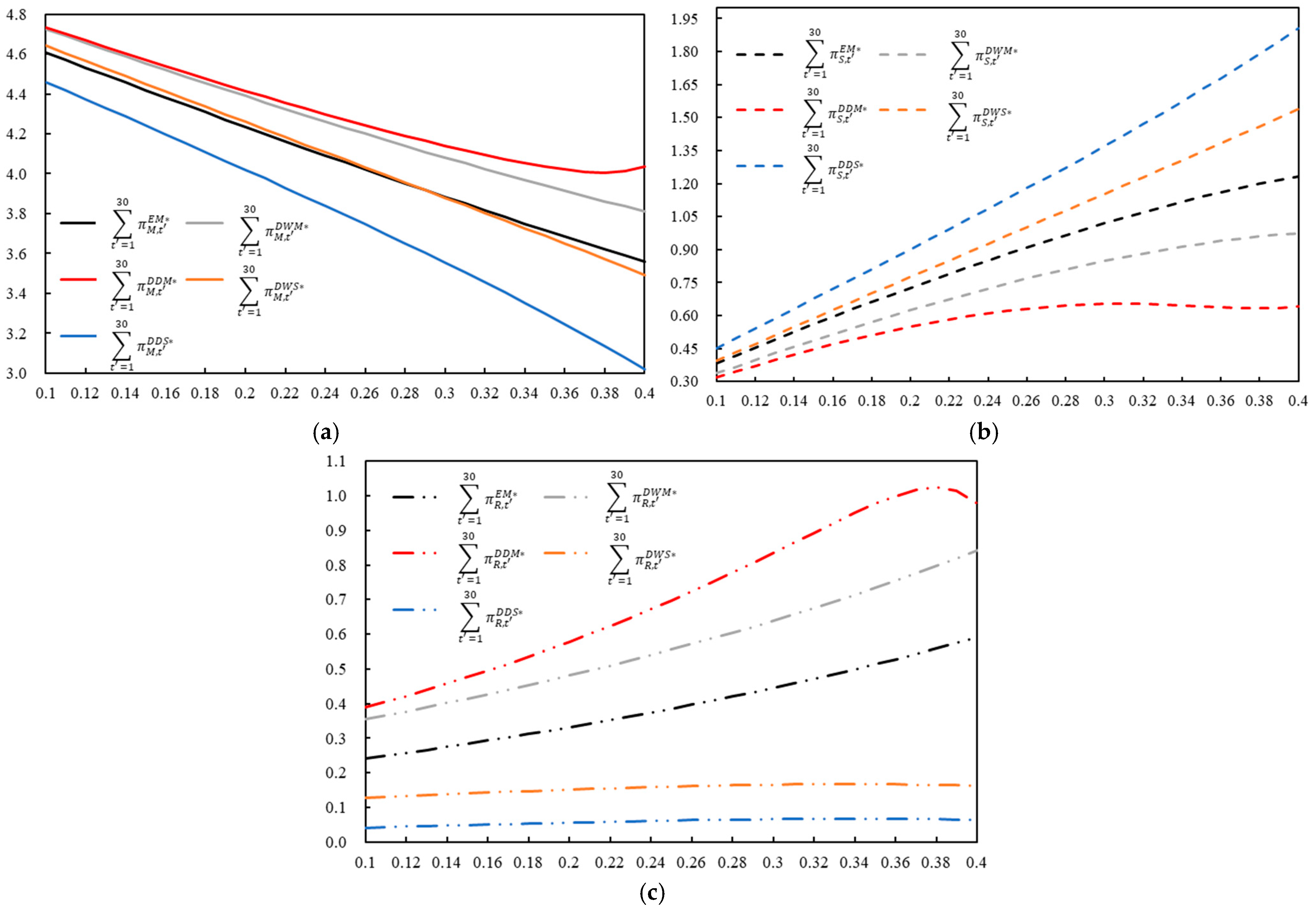
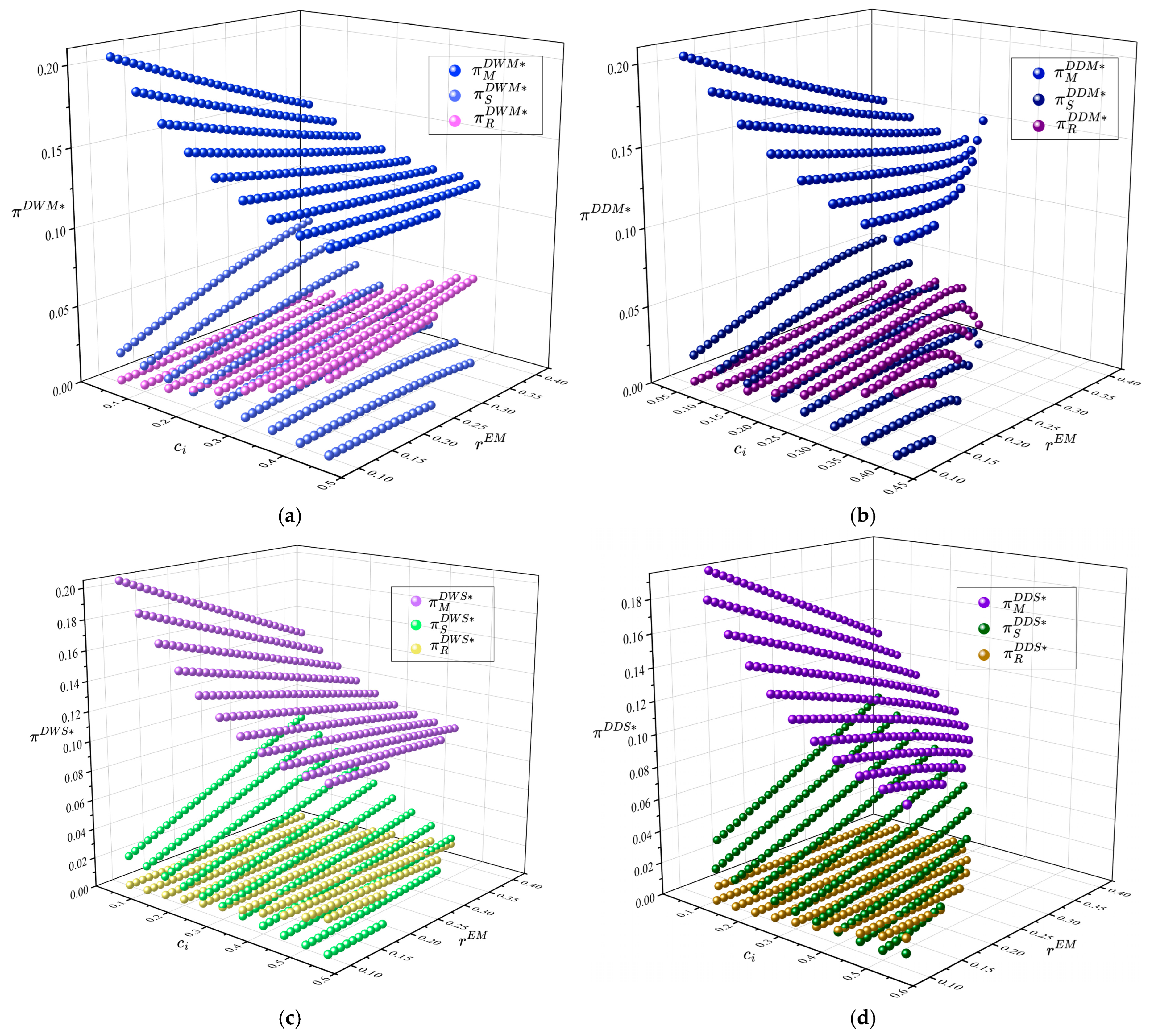
5.1. Comparison Among Dynamic Models

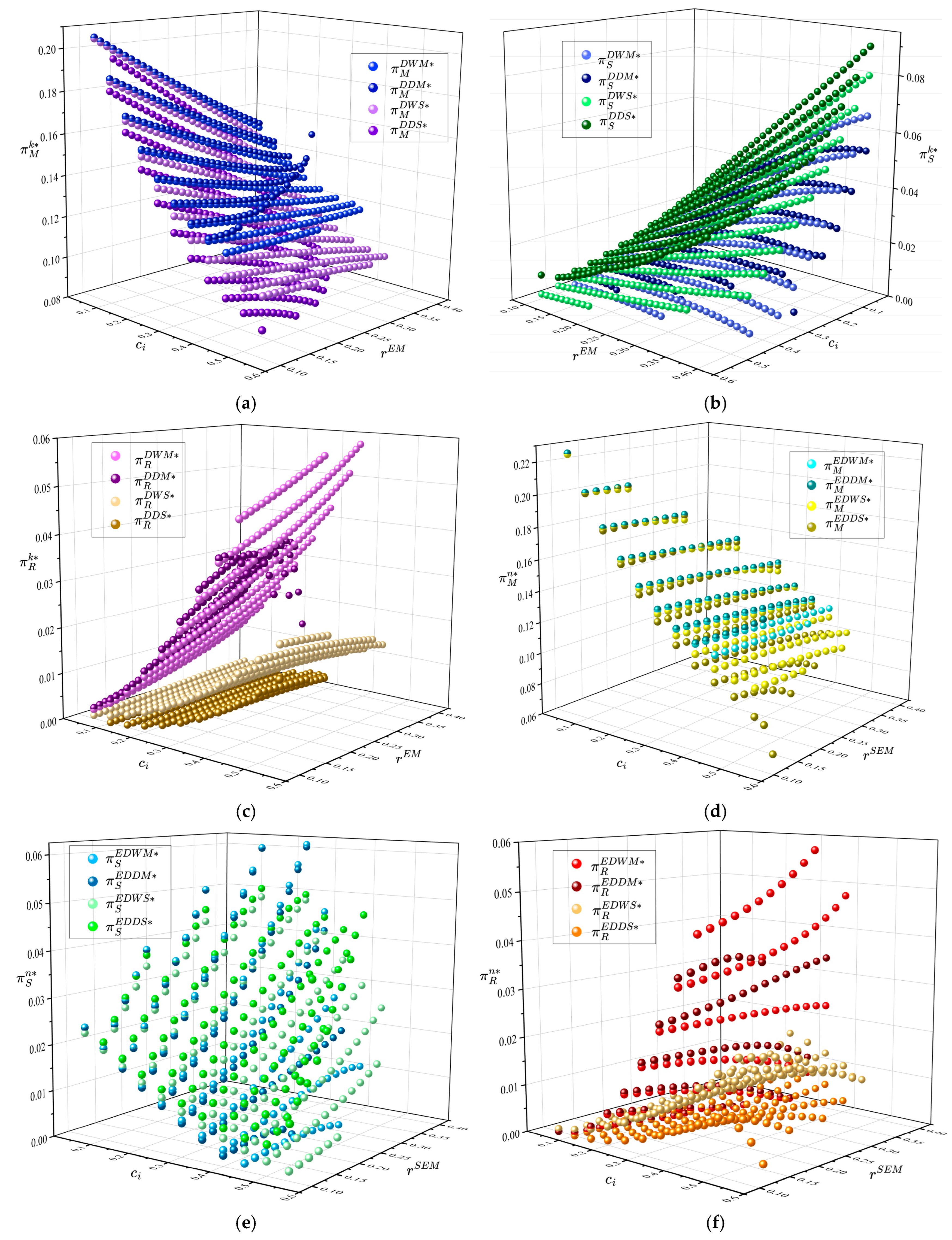
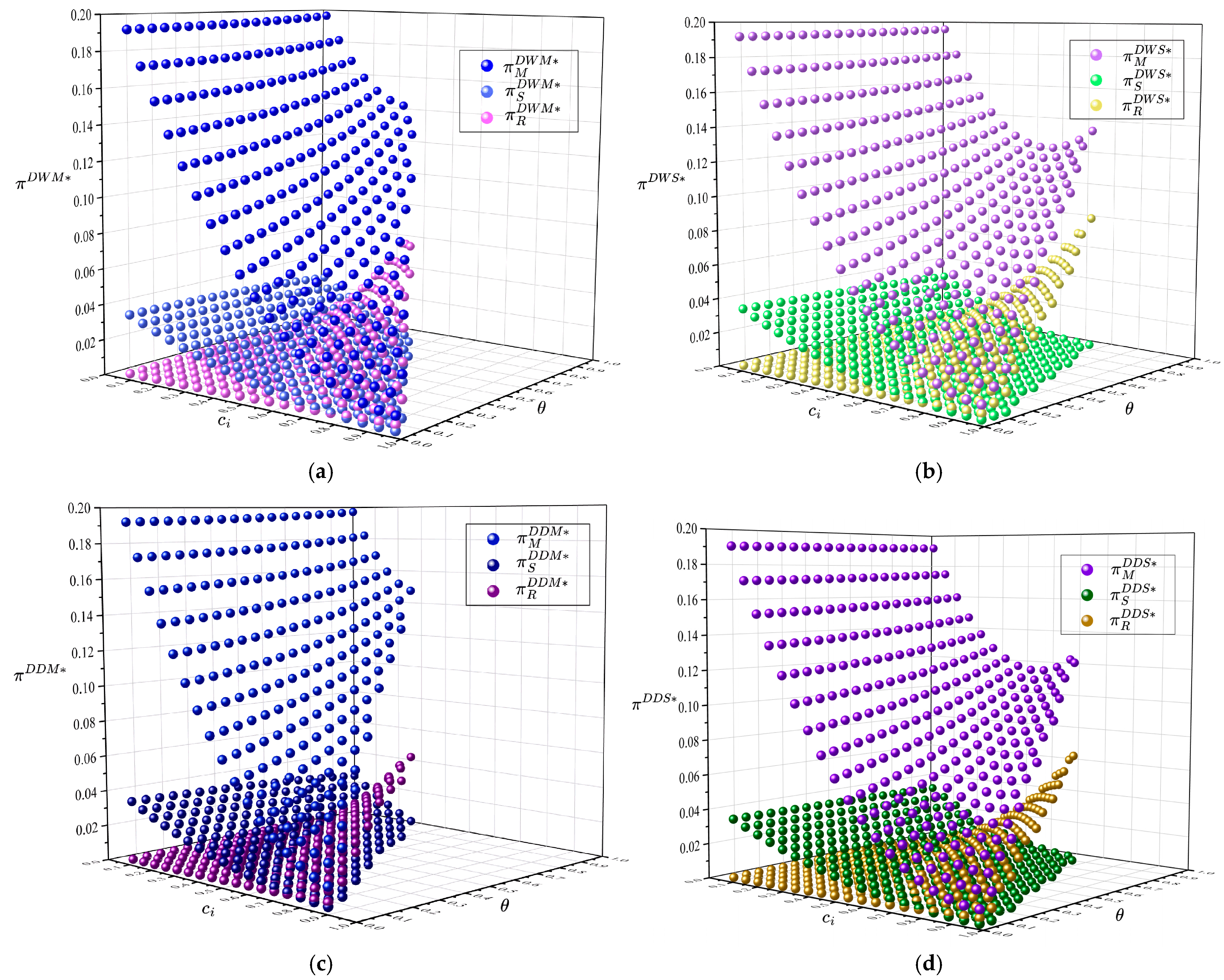
We begin by analyzing the commission preferences of the manufacturer, streamer, and retailer under a uniform rate, $r_1^{DWM}=r_1^{DDM}=r_1^{DWS}=r_1^{DDS}=r^{EM}$. Using the optimal outcomes from the exogenous model, we conduct a dynamic analysis with 40 initial states, varying the commission rate from 0.1 to 0.4 [20]. The parameters are fixed as follows: $c_i=0.2$, $a=10$. Following [50,63], we set $\theta =0.8$ and $\alpha =0.8$. By examining total profits over 30 periods, we aim to identify the commission structure that maximizes profitability for each party.

Figure 2 supports Proposition 4 and reveals two important findings regarding the influence of the initial commission rate on commission structure choices. First, both the manufacturer and streamer prefer a weaker partner when in dominant roles. The retailer consistently aligns with the manufacturer, indicating a shared interest. Second, the dominant role influences the choice of dynamic commission structure. Specifically, for the manufacturer and streamer, the preference order of the commission structure is dual-dynamic of dominance > dynamic wholesale price of dominance > dynamic wholesale price of non-dominance > dual-dynamic of non-dominance.

Figure 3 illustrates the steady trends of decision variables concerning the selling ease via the live-stream channel at various initial commission rates. While the spillover effect and initial commission rate do not affect these trends, dominant roles significantly influence them. These variations arise from the adjustment strategies of the manufacturer, streamer, and retailer under different power structures, as outlined in Lemmas 2 and 4. In manufacturer-dominating scenarios, the steady-state commission rate and wholesale price decline under dynamic mechanisms. Conversely, in streamer-dominating scenarios, the commission rate and wholesale price increase as the manufacturer compensates for losses in the live-stream channel. The retailer, impacted by the dynamic wholesale price, continuously seeks to boost sales in the traditional online channel. Overall, live-stream channel sales decrease across all models due to strategic choices made by the manufacturer and streamer in their respective dominant roles.

Figure 3 shows how hassle cost and initial commission rate affect decision variables in steady states. Correspondingly, Figure 4 identifies the optimal initial commission rate for products with different selling difficulties. It also highlights how these selling difficulties, along with initial commission rates, shape the commission structure preferences of the manufacturer, streamer, and retailer.

Figure 4 supports Proposition 5 and Figure 2 by guiding the setting of the initial commission rate for products with varying selling difficulties under different commission structures. In manufacturer-dominating scenarios, both the manufacturer and retailer prefer the dual dynamic model, as the manufacturer controls the live-stream channel and dynamic commission rate. Conversely, in streamer-dominating scenarios, the dynamic wholesale price model becomes more favorable, with the streamer taking the lead. This numerical experiment validates Proposition 6 and reinforces Figure 2 by comparing all four models, offering joint recommendations for partner selection and commission structure. The preferences align with Figure 2: the manufacturer favors DWM and DDM, while the streamer prefers DWS and DDS, prioritizing dual dynamic models. When the other party holds an advantage, they lean toward single dynamic models. Specifically, the manufacturer prefers DDM, followed by DWM, DWS, and lastly DDS. The streamer prefers DDS, followed by DWS, DWM, and DDM. Consistent with Propositions 3, 4, and 5, the retailer generally aligns with the manufacturer’s preferences, except in cases of high commission rates, where the dynamic wholesale price may be more beneficial for the retailer than a dual dynamic commission. Nonetheless, this scenario is still more favorable than streamer-dominating situations.

Figure 4d–f reveal how the positive spillover effect impacts strategic commission structure decisions. When the spillover effect is considered, the initial commission rate and hassle cost are key factors in determining preferences for the manufacturer, streamer, and retailer. For the manufacturer, EDDM consistently outperforms EDWM and the streamer-dominating models (EDWS and EDDS). As the initial commission rate rises, especially for products with medium and lower selling difficulty, EDDS becomes more favorable than EDWS, contrasting with preferences without the spillover effect. For the streamer, EDDS is preferred over EDWS, and EDWM is favored over EDDM. In particular, manufacturer-dominating structures like EDWM and EDDM are more advantageous for moderately easy and easy-to-sell products at higher initial commission rates. The retailer prefers EDDM over EDWM and EDWS over EDDS. As products become easier to sell and the initial commission rate rises, streamer-dominating structures (EDWS and EDDS) become more favorable.

5.2. Product Type

This section examines product types that yield favorable outcomes for the manufacturer, retailer, and streamer under different parameter settings. Within the DWM model in Figure 5, the manufacturer’s profit declines for products that are difficult to sell via live-stream but advantageous through traditional online channels. The streamer faces diminished profit as live-stream selling difficulty increases, while the retailer suffers when live-stream sales are easy. Figure 5a shows that the manufacturer’s and streamer’s profit decreases are significantly influenced by hassle cost, as is the retailer’s profit increase. Thus, to satisfy all profit margins, hassle cost should be moderate, and the disutility factor should be mid to high. The DDM model findings are closely similar to DWM, indicating that commission structures have little effect on product preferences for the manufacturer, streamer, and retailer. In the DWS model, the manufacturer’s profit initially falls but eventually rises with a high hassle cost and a high disutility factor. Although the retailer and streamer aim to maximize profits under streamer-dominating dynamic wholesale pricing, the live-stream channel’s advantage weakens as hassle cost increases. Consequently, the manufacturer’s profit growth from the traditional online channel cannot compensate for live-stream losses. However, as the live-stream losses diminish and traditional online profits increase due to a high disutility factor, the manufacturer’s overall profitability improves. For the DWS and DDS models, the optimal product types for joint profitability are those with a mid to high disutility factor and moderate hassle cost.

For the DWM model in Figure 6, the manufacturer experiences reduced profit for hard-to-sell product in a live-stream channel. Similarly, the streamer’s profit also diminishes in these cases, while the retailer’s profits decline when live-stream sales are easier. Figure 6a shows that the manufacturer’s and streamer’s profit reductions are significantly influenced by hassle cost, as is the retailer’s profit increase. Therefore, maintaining a moderate hassle cost is key to preserving overall profitability. The DDM model presents a contrast to the DWM model. For products that are difficult to sell through the live-stream channel, a higher initial commission rate can substantially boost the manufacturer’s profit under the dual dynamic model. However, the retailer’s profit is significantly reduced in this scenario. Profit changes for the streamer and manufacturer align with the DWM model. As product sales difficulty varies, the profits of the manufacturer and streamer become more volatile. In contrast, the retailer’s profit remains relatively stable, showing a slight increase with increased sales difficulty. The retailer’s profit is unaffected by hassle cost and the initial commission rate. Although the retailer’s profit remains relatively stable across parameter variations in the DWS and DDS analyses, it is still beneficial to maintain a moderate hassle cost and initial commission rate to ensure satisfactory profits for all three parties involved.

Figure 7 shows the choice of product type that gains higher joint profits, taking into account the spillover effect. In manufacturer-dominating scenarios, the retailer’s profit fluctuations are more distinctly influenced by hassle cost and initial commission rate. The profit trends for the manufacturer, streamer, and retailer are similar to those in scenarios without the spillover effect. Conversely, in streamer-dominating scenarios, the retailer’s profit is less sensitive to parameter changes, while the profit trends for the manufacturer and streamer remain consistent.

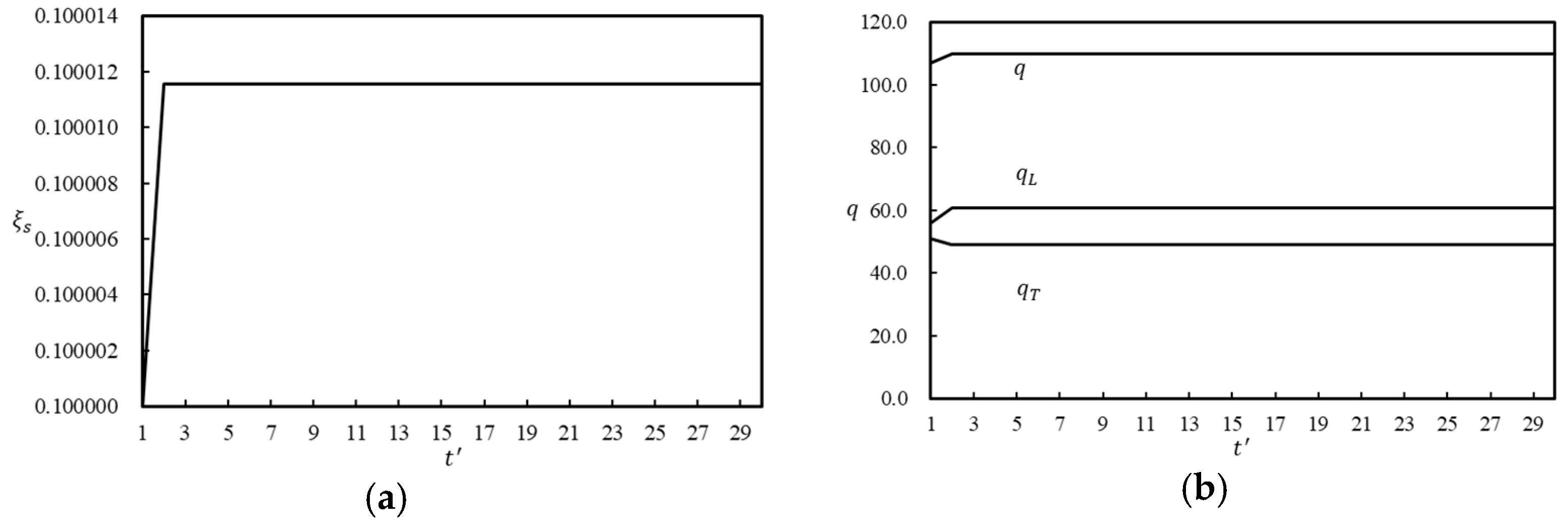
5.3. Validation of Dynamic Commission Rate

To verify the superiority and practicability of the dynamic commission rate, we cite numerical experiments based on [25] by applying the dynamic commission rate to the live-stream model S. Fixed parameters are exactly same as in the study by [25], except for the commission rate charged by the streamer. We obtain the commission rate of the streamer for each period, traditional channel sales, live-stream channel sales, and total sales, as shown in Figure 8.

Figure 8 presents the streamer’s commission rate over period $t^{\prime }$ after applying the dynamic commission rate. The streamer is incentivized by the commission rate to increase sales in the live-stream channel, which, in turn, raises the commission rate. Meanwhile, the manufacturer increases total sales despite a reduction in traditional channel sales. As demonstrated in Figure 8, the total sales across the dual-channel system increase.

6. Conclusions Summary

6.1. Conclusions

This study examines optimal strategies for the manufacturer, streamer, and retailer under two power structures—manufacturer-dominating and streamer-dominating—and across three commission structures: exogenous, dynamic wholesale price, and synergistic dual dynamic. We conducted a comparative analysis of six models to examine how factors like hassle cost, disutility, and initial commission rate influence partnership and commission decisions, aiming to maximize profitability for all parties.

Firstly, the comparative analysis of multiple models reveals that the manufacturer and retailer tend to share similar interests when choosing commission structures, particularly under manufacturer-dominating scenarios. Dynamic models generally lead to higher profits for both parties, whereas the streamer often prefers the benchmark model due to a weaker position in such power structures. In streamer-dominating scenarios, dynamic wholesale pricing remains beneficial for the manufacturer and retailer, while the streamer finds profitability more challenging, often favoring exogenous models instead.

Secondly, fixing the disutility factor highlights how hassle cost and initial commission rate shape the choices of commission structures and product types. Moderate hassle costs and initial commission rates create a win–win situation, benefiting all parties. The analysis confirms that manufacturers in a dominant position favor dual dynamic commission, while those in a follower role prefer single dynamic commissions. Importantly, this approach helps identify the reasonable range of initial commission rates that ensure joint profitability across different product categories.

Thirdly, examining partner selection under identical commission rates shows that both the manufacturer and streamer tend to prefer less influential partners. Retailers often align their choices with the manufacturer’s preferences, indicating a strong convergence of interests. This alignment fosters better collaboration among the three parties, resulting in improved profitability and more stable partnerships over time.

Lastly, the interplay between dynamic wholesale prices and dynamic commission rates yields distinct outcomes. In manufacturer-dominating scenarios, dynamic wholesale pricing significantly benefits the manufacturer and retailer but reduces streamer profits. Conversely, dynamic commission rates can positively impact the streamer in streamer-dominating contexts, even as their effect on the manufacturer and retailer is less favorable. Notably, all dynamic models eventually converge to a steady state, providing a reliable foundation for sustainable, long-term collaborations.

6.2. Managerial Insights

(i)

When selecting the appropriate commission structure, manufacturers operating in manufacturer-dominated scenarios can significantly improve their profits by adopting dynamic wholesale pricing or a dual dynamic mechanism. This approach also benefits retailers, as collaborative alignment increases overall efficiency. However, manufacturers should be mindful that dynamic commission rates may diminish the incentives for streamers in the live-streaming channel, potentially affecting long-term channel performance.

(ii)

In terms of product type and channel management, choosing products with moderate hassle costs and a higher disutility factor proves advantageous. Such products enhance the manufacturer’s profits by optimizing performance across both live-stream and traditional channels. Balancing these product characteristics helps ensure that channel management strategies are effective and contribute to sustained profitability.

(iii)

For partner selection, manufacturers generally favor L-streamers. This preference enables them to reduce commission costs while retaining stronger control over the traditional retail channel. By partnering with less influential streamers, manufacturers can achieve better coordination and maximize profits across both live-stream and traditional sales channels.

(iv)

The dual effect of dynamic mechanisms must also be carefully considered. While dynamic wholesale prices reliably contribute to the manufacturer’s profitability, dynamic commission rates can have adverse effects under certain conditions. Manufacturers must thoroughly evaluate these combined effects to determine the best approach to maximizing overall profits and sustaining channel growth.

(v)

Lastly, the stability of long-term partnerships is reinforced by the fact that all dynamic models eventually reach a steady state. This convergence not only ensures long-term supply chain sustainability but also provides a predictable foundation for ongoing profitability. Manufacturers should leverage these dynamic adjustments to maintain stable partnerships and foster a resilient supply chain over time.

6.3. Limitations

In this paper, we unify the memory parameter in dynamic models for both dynamic wholesale price and dynamic commission rate. Future research will differentiate memory parameters for these dynamic elements to examine their distinct impacts on the decisions of the manufacturer, streamer, and retailer regarding commission structures and power structures. Additionally, while this study only considers positive spillover effect moderated by live-stream hassle cost, subsequent work will investigate the influence of both negative and positive spillover effects on decision-making.

Our findings are derived from theoretical analyses and thus lack direct empirical validation, representing a limitation of this study. Future research could empirically test our proposed dynamic pricing and commission structures using real-world data from live-stream e-commerce platforms to enhance the practical applicability and robustness of the results.

References

1. Wongkitrungrueng, A.; Assarut, N. The role of live streaming in building consumer trust and engagement with social commerce sellers. J. Bus. Res. 2020, 117, 543–556. [Google Scholar]
2. Chen, H.; Dou, Y.; Xiao, Y. Understanding the Role of Live Streamers in Live-Streaming E-Commerce. Electron. Commer. Res. Appl. 2023, 59, 101266. [Google Scholar]
3. Pan, R.; Feng, J.; Zhao, Z. Fly with the wings of live-stream selling—Channel strategies with/without switching demand. Prod. Oper. Manag. 2022, 30, 3387–3399. [Google Scholar]
4. Zhang, Z.; Chen, Z.; Wan, M.; Zhang, Z. Dynamic quality management of live streaming e-commerce supply chain considering streamer type. Comput. Ind. Eng. 2023, 182, 109357. [Google Scholar] [CrossRef]
5. Thepaper. 2024. Available online: https://www.thepaper.cn/newsDetail_forward_27890414 (accessed on 29 June 2024).
6. Agri.cn. Available online: http://www.agri.cn/sj/jcyj/ (accessed on 25 March 2025).
7. Mbalib.com. Available online: https://www.mbalib.com/ask/question-6bdf2e72435e2ef4bad7aaf556c33d1e.html (accessed on 15 February 2025).
8. Toutiao. 2024. Available online: https://www.toutiao.com/article/7424452540441428519/ (accessed on 11 October 2024).
9. Qu, Y. Judicial Empirical Research on Disputes over Online Live Streaming with Goods. Acad. J. Bus. Manag. 2023, 5, 96–104. [Google Scholar]
10. Simchi-Levi, D.; Zheng, Z.; Zhu, F. Offline Planning and Online Learning Under Recovering Rewards. Manag. Sci. 2024, 71, 298–317. [Google Scholar]
11. Lu, S.; Yao, D.; Chen, X.; Grewal, R. Do Larger Audiences Generate Greater Revenues under Pay What You Want? Evidence from a Live-stream Platform. Manag. Sci. 2021, 40, 813–1007. [Google Scholar]
12. Zhao, K.; Lu, Y.; Hu, Y.; Hong, Y. Direct and indirect spillovers from content providers’ switching: Evidence from online livestreaming. Inf. Syst. Res. 2023, 34, 847–866. [Google Scholar]
13. Kang, K.; Lu, J.; Guo, L.; Li, W. The dynamic effect of interactivity on customer engagement behavior through tie strength: Evidence from live streaming commerce platforms. Int. J. Inf. Manag. 2021, 56, 102251. [Google Scholar]
14. Cui, X.; Li, Y.; Li, X.; Fang, S. Livestream e-commerce in a platform supply chain: A product-fit uncertainty reduction perspective. Int. J. Prod. Econ. 2023, 258, 108796. [Google Scholar]
15. Xie, P.; Shi, R.; Xu, D. Retailer service strategy on livestreaming platforms considering free riding behavior. Ann. Oper. Res. 2023, 344, 647–677. [Google Scholar]
16. Huang, L.; Liu, B.; Zhang, R. Channel strategies for competing retailers: Whether and when to introduce live stream? Eur. J. Oper. Res. 2024, 312, 413–426. [Google Scholar] [CrossRef]
17. Zhang, W.; Liu, C.W.; Ming, L.; Cheng, Y. The sales impacts of traffic acquisition promotion in live-stream commerce. Prod. Oper. Manag. 2024. [Google Scholar] [CrossRef]
18. Hou, J.; Shen, H.; Xu, F. A Model of Livestream Selling with Online Influencers. Soc. Sci. Res. Netw. 2021. [Google Scholar] [CrossRef]
19. Ji, G.; Fu, T.; Li, S. Optimal selling format considering price discount strategy in live-streaming commerce. Eur. J. Oper. Res. 2023, 309, 529–544. [Google Scholar]
20. Hao, C.; Yang, L. Resale or Agency Sale? Equilibrium Analysis on the Role of Live-stream Selling. Eur. J. Oper. Res. 2023, 307, 1117–1134. [Google Scholar]
21. Wang, J.; Zhang, X. The value of influencer channel in an emerging livestreaming e-commerce model. J. Oper. Res. Soc. 2023, 74, 112–124. [Google Scholar] [CrossRef]
22. Huang, M.X.; Ye, Y.Q.; Wang, W. The interaction effect of broadcaster and product type on consumers’ purchase intention and behaviors in livestreaming shopping. Nankai Bus. Rev. 2021, 26, 188–198. [Google Scholar]
23. Niu, B.; Chen, Y.; Zhang, J.; Chen, K.; Jin, Y. Brands’ Livestream Selling with Influencers’ Converting Fans into Consumers. Omega 2024, 131, 103195. [Google Scholar] [CrossRef]
24. Ye, F.; Ji, L.; Ning, Y.; Li, Y. Influencer selection and strategic analysis for live streaming selling. J. Retail. Consum. Serv. 2024, 77, 103673. [Google Scholar] [CrossRef]
25. Zhang, W.; Yu, L.; Wang, Z. Live-streaming selling modes on a retail platform. Transp. Res. Part E Logist. Transp. Rev. 2023, 173, 103096. [Google Scholar]
26. Qi, A.; Sethi, S.; Wei, L.; Zhang, J. Top or regular influencer? Contracting in live streaming platform selling. Soc. Sci. Res. Netw. 2022. [Google Scholar] [CrossRef]
27. Wang, X.; Tao, Z.; Liang, L.; Gou, Q. An analysis of salary mechanisms in the sharing economy: The interaction between streamers and unions. Int. J. Prod. Econ. 2019, 214, 106–124. [Google Scholar]
28. Yang, X.; Gou, Q.; Wang, X.; Zhang, J. Does bonus motivate streamers to perform better? An analysis of compensation mechanisms for live-stream platforms. Transp. Res. Part E Logist. Transp. Rev. 2022, 164, 102758. [Google Scholar]
29. Liu, S.; Hua, G.; Cheng, T.E.; Choi, T.M. Optimal pricing and quality decisions in supply chains with consumers’ anticipated regret and online celebrity retailers. IEEE Trans. Eng. Manag. 2024, 71, 1115–1129. [Google Scholar]
30. Huang, H.; Ke, H.; Wang, L. Equilibrium analysis of pricing competition and cooperation in supply chain with one common manufacturer and duopoly retailers. Int. J. Prod. Econ. 2016, 178, 12–21. [Google Scholar]
31. Li, G.; Li, L.; Liu, M.; Sethi, S.P. Impact of power structures in a subcontracting assembly system. Ann. Oper. Res. 2020, 291, 475–498. [Google Scholar]
32. Hu, Y.; Qu, S.; Li, G.; Sethi, S.P. Power structure and channel integration strategy for online retailers. Eur. J. Oper. Res. 2021, 294, 951–964. [Google Scholar]
33. Chen, Z.; Fan, Z.-P.; Zhao, X. Offering return-freight insurance or not: Strategic analysis of an e-seller’s decisions. Omega 2021, 103, 102447. [Google Scholar]
34. Zhang, Z.; Xu, H.; Chen, K.; Zhao, Y.; Liu, Z. Channel mode selection for an e-platform supply chain in the presence of a secondary marketplace. Eur. J. Oper. Res. 2023, 305, 1215–1235. [Google Scholar]
35. Tian, L.; Vakharia, A.J.; Tan, Y.; Xu, Y. Marketplace, reseller, or hybrid: Strategic analysis of an emerging e-commerce model. Prod. Oper. Manag. 2018, 28, 1595–1610. [Google Scholar]
36. Yan, Y.; Zhao, R.; Xing, T. Strategic introduction of the marketplace channel under dual upstream disadvantages in sales efficiency and demand information. Eur. J. Oper. Res. 2019, 273, 968–982. [Google Scholar]
37. Liu, H.; Xu, T.; Jing, S.; Liu, Z.; Wang, S. The interplay between logistics strategy and platform’s channel structure design in b2c platform market. Eur. J. Oper. Res. 2023, 310, 812–833. [Google Scholar]
38. Geng, X.; Tan, Y.; Wei, L. How add-on pricing interacts with distribution contracts. Prod. Oper. Manag. 2018, 27, 605–623. [Google Scholar]
39. Ha, A.Y.; Tong, S.; Wang, Y. Channel structures of online retail platforms. Manuf. Serv. Oper. Manag. 2022, 24, 1547–1561. [Google Scholar]
40. Zhen, X.; Xu, S.; Li, Y.; Shi, D. When and how should a retailer use third-party platform channels? the impact of spillover effects. Eur. J. Oper. Res. 2022, 301, 624–637. [Google Scholar]
41. Wei, J.; Lu, J.; Zhao, J. Interactions of competing manufacturers’ leader-follower relationship and sales format on online platforms. Eur. J. Oper. Res. 2019, 280, 508–522. [Google Scholar]
42. Li, L.; Fang, X.; Lim, Y.F. Asymmetric information of product authenticity on c2c e-commerce platforms: How can inspection services help? Manuf. Serv. Oper. Manag. 2023, 25, 631–647. [Google Scholar]
43. Hu, H.; Zheng, Q.; Pan, X.A. Agency or wholesale? The role of retail pass-through. Manag. Sci. 2022, 68, 7538–7554. [Google Scholar]
44. Wei, Y.; Dong, Y. Product distribution strategy in response to the platform’s marketplace introduction. Eur. J. Oper. Res. 2022, 303, 886–896. [Google Scholar]
45. Wang, L.; Chen, J.; Song, H. Marketplace or reseller? platform strategy in the presence of customer returns. Transp. Res. Part E Logist. Transp. Rev. 2021, 153, 102452. [Google Scholar] [CrossRef]
46. Abhishek, V.; Jerath, K.; Zhang, Z.J. Agency selling or reselling? Channel structures in electronic retailing. Manag. Sci. 2016, 62, 2259–2280. [Google Scholar]
47. Yang, L.; Guo, J.; Zhou, Y.W.; Cao, B. Equilibrium analysis for competing o2o supply chains with spillovers: Exogenous vs. endogenous consignment rates. Comput. Ind. Eng. 2021, 162, 107690. [Google Scholar] [CrossRef]
48. Tsunoda, Y.; Zennyo, Y. Platform information transparency and effects on third–party suppliers and offline retailers. Prod. Oper. Manag. 2021, 30, 4219–4235. [Google Scholar] [CrossRef]
49. Liu, W.; Yan, X.; Li, X.; Wei, W. The impacts of market size and data-driven marketing on the sales mode selection in an internet platform based supply chain. Transp. Res. Part E Logist. Transp. Rev. 2020, 136, 101914. [Google Scholar] [CrossRef]
50. Popescu, I.; Wu, Y. Dynamic pricing strategies with reference effects. Oper. Res. 2007, 55, 413–429. [Google Scholar]
51. Chen, X.; Hu, P.; Shum, S.; Zhang, Y. Dynamic stochastic inventory management with reference price effects. Oper. Res. 2016, 64, 1529–1536. [Google Scholar] [CrossRef]
52. Wang, Z. Technical note–intertemporal price discrimination via reference price effects. Oper. Res. 2016, 64, 290–296. [Google Scholar] [CrossRef]
53. Cao, P.; Zhao, N.; Wu, J. Dynamic pricing with bayesian demand learning and reference price effect. Eur. J. Oper. Res. 2019, 279, 540–556. [Google Scholar] [CrossRef]
54. Zhao, N.; Wang, Q.; Cao, P.; Wu, J. Dynamic pricing with reference price effect and price-matching policy in the presence of strategic consumers. J. Oper. Res. Soc. 2019, 70, 2069–2083. [Google Scholar] [CrossRef]
55. Zhang, J.; Chiang, W.-Y.K. Durable goods pricing with reference price effects. Omega 2020, 91, 102018. [Google Scholar]
56. Chen, J.; Pun, H.; Zhang, Q. Eliminate demand information disadvantage in a supplier encroachment supply chain with information acquisition. Eur. J. Oper. Res. 2023, 305, 659–673. [Google Scholar] [CrossRef]
57. Tang, Y.; Sethi, S.P.; Wang, Y. Games of supplier encroachment channel selection and e-tailer’s information sharing. Prod. Oper. Manag. 2023, 32, 3650–3664. [Google Scholar] [CrossRef]
58. Sun, S.; Zheng, X.; Sun, L. Multi-period pricing in the presence of competition and social influence. Int. J. Prod. Econ. 2020, 227, 107662. [Google Scholar] [CrossRef]
59. Chen, K.; Zha, Y.; Alwan, L.C.; Zhang, L. Dynamic pricing in the presence of reference price effect and consumer strategic behaviour. Int. J. Prod. Res. 2019, 58, 546–561. [Google Scholar] [CrossRef]
60. Chen, Q.; Yan, X.; Bian, Y.; Han, X. Live Streaming Channel and Product Assortment with both National and Store Brand products. Omega 2024, 131, 103212. [Google Scholar]
61. Yu, T.; Guan, Z.; Dong, J. Research on Live E-Commerce Supply Chain Decision-Making Considering Social Media Influencer’s Marketing Efforts under Different Power Structures. Chin. J. Manag. 2022, 19, 714–722. [Google Scholar]
62. Li, Y.; Ning, Y.; Fan, W.; Kumar, A.; Ye, F. Channel Choice in Live Streaming Commerce. Prod. Oper. Manag. 2024, 11, 2221–2240. [Google Scholar] [CrossRef]
63. Li, S.L.; Kenneth, C.H.; Yong, J. Optimal distribution strategy for enterprise software: Retail, saas, or dual channel? Prod. Oper. Manag. 2018, 27, 1928–1939. [Google Scholar]
64. Matsui, K. Optimal bargaining timing of a wholesale price for a manufacturer with a retailer in a dual-channel supply chain. Eur. J. Oper. Res. 2020, 287, 225–236. [Google Scholar]
65. Shen, B.; Xu, X.; Guo, S. The impacts of logistics services on short life cycle products in a global supply chain. Transp. Res. Part E Logist. Transp. Rev. 2019, 131, 153–167. [Google Scholar]
66. Dong, S.; Qin, Z.; Yan, Y. Effects of online-to-offline spillovers on pricing and quality strategies of competing firms. Int. J. Prod. Econ. 2022, 244, 108376. [Google Scholar]
67. Hsieh, C.; Lathifah, A. Exploring the spillover effect and supply chain coordination in dual-channel green supply chains with blockchain-based sales platform. Comput. Ind. Eng. 2023, 187, 109801. [Google Scholar]
68. Yang, W.; Govindan, K.; Zhang, J. Spillover effects of live streaming selling in a dual-channel supply chain. Transp. Res. Part E Logist. Transp. Rev. 2023, 180, 103298. [Google Scholar]
Figure 1. The sequence of events under dynamic models.
Jtaer 20 00061 g001
Figure 2. Profits in dynamic models. (a) The manufacturer’s profits; (b) the streamer’s profits; (c) the retailer’s profits.
Jtaer 20 00061 g002
Figure 3. Steady states of variables in dual dynamic models. (a) Variables in the DDM model; (b) variables in the EDDM model; (c) variables in the DDS model; (d) variables in the EDDS model.
Jtaer 20 00061 g003
Figure 4. Comparison of dynamic models ( τ S E M P = 0.06 ). (a) The profits of the manufacturer; (b) the profits of the streamer; (c) the profits of the retailer; (d) the profits of the manufacturer; (e) the profits of the streamer; (f) the profits of the retailer.
Jtaer 20 00061 g004
Figure 5. The option of product type in dynamic models (with r E M = r E S = 0.15 ). (a) The choice in the DWM model; (b) the choice in the DWS model; (c) the choice in the DDM model; (d) the choice in the DDS model.
Jtaer 20 00061 g005
Figure 6. The option of product type in dynamic models (with θ = 0.8 ). (a) The choice in the DWM model; (b) the choice in the DWS model; (c) the choice in the DDM model; (d) the choice in the DDS model.
Jtaer 20 00061 g006
Figure 7. The option of product type in extended models. (a) The choice in the EDWM model; (b) the choice in the EDDM model; (c) the choice in the EDWS model; (d) the choice in the EDDS model.
Jtaer 20 00061 g007
Figure 8. The commission rate and channel sales in [25]. (a) The streamer’s commission rate; (b) the sales.
Jtaer 20 00061 g008