Abstract
In this paper, a hybrid model that considers both accuracy and efficiency is proposed to predict photovoltaic (PV) power generation. To achieve this, improved forward feature selection is applied to obtain the optimal feature set, which aims to remove redundant information and obtain related features, resulting in a significant improvement in forecasting accuracy and efficiency. The prediction error is irregularly distributed. Thus, a bias compensation–long short-term memory (BC–LSTM) network is proposed to minimize the prediction error. The experimental results show that the new feature selection method can improve the prediction accuracy by 0.6% and the calculation efficiency by 20% compared to using feature importance identification based on LightGBM. The BC–LSTM network can improve accuracy by 0.3% using about twice the time compared with the LSTM network, and the hybrid model can further improve prediction accuracy and efficiency based on the BC–LSTM network.
1. Introduction
Currently, the consumption of fossil energy is increasing with societal developments. Solar energy has received more and more attention from all over the world in the past decade [1]. More and more PV power plants connected to the grid will bring great challenges to its security and stability [2,3]. In the case of the poor prediction accuracy of a PV power outage, the spinning reserve of a conventional power supply has to be increased to ensure the safety of the power system. As a result, the renewable energy consumption space is crowded out, which results in an increase in the amount of abandoned sunlight. Accurate forecasting of PV power generation can provide a reliable basis for peak load and frequency regulation, power flow optimization, and equipment maintenance, as well as technical support for the complementary and coordinated control of wind power, which is one of the key technologies to improve the grid’s ability to accept PV power. Therefore, accurate and reliable PV forecasting techniques are needed to optimize operation costs and reduce uncertainties in power systems [4].
The approaches of PV power prediction are generally divided into two categories: stepwise methods and direct methods [5]. The stepwise forecast consists of two steps. First, solar radiation intensity [6,7,8,9,10] and temperature [11,12,13] are forecasted, which are then applied as inputs to forecast the PV power. Unlike the stepwise forecast method, direct forecast predicts PV power through the historical data of PV power and meteorological information, and its approaches are divided into three categories: (1) statistical model methods; (2) physical methods; and (3) artificial intelligent learning methods [14,15,16].
One common method to improve prediction efficiency and accuracy is to select the optimal feature set from the original data set [17,18,19,20]. One way to select the optimal feature set is to use the Pearson correlation coefficient to analyze the influence of various meteorological factors on the output of PV power generation [21]. The Pearson coefficient can analyze linear relationships between features, but its ability to analyze nonlinear or nonstationary problems is limited. To better solve nonlinear or nonstationary problems, some researchers proposed an adaptive hybrid predictor subset selection strategy to obtain the most relevant and nonredundant predictors for enhanced short-term forecasting [22]. The strategy chooses the optimal feature set through the following two aspects: (1) the correlation between features and PV power to choose the most relevant feature set, and (2) the correlation between features to select the nonredundant feature set. However, according to our research, some features alone will not affect the prediction results, but a combination of certain features can affect the prediction results. We call this feature a combination relationship. Based on the existing research, we propose a new feature selection method, designed in consideration of all three aforementioned aspects.
Another common method to improve prediction accuracy is to change the structure of the model [23,24,25,26,27,28]. The convolutional neural network (CNN) embodies powerful capabilities in image processing [29]. In recent years, more and more CNN-based models have been used to forecast PV power and have achieved good results. The CNN network can extract the features of the original data well, but it is not good at dealing with timing problems. A recurrent neural network (RNN) is considered to be a more effective tool for time series data prediction. In previous work, some researchers demonstrated that RNN has better prediction performance than backpropagation NN (BPNN) and radial basis function NN (RBFNN) [30,31]. Unlike the aforementioned studies, some researchers introduced the concept of residuals into the model design [32]. By establishing an additional error prediction model, the prediction error is added back to the prediction result to obtain the final prediction result. This method cleverly introduces error compensation terms to improve prediction accuracy. Based on this, and considering the superiority of LSTM networks in time series problems, a hybrid model, the bias compensation–long short-term memory (BC–LSTM) network, is used to perform the PV power forecasting.
However, traditional bias compensation networks have the following problems. The actual power value and the power error term are generated inconsistently, and the influencing factors are also different. Using the same meteorological data as the model input, its prediction accuracy is poor, and its computational complexity is high. Therefore, a framework with a hybrid method combining feature selection and the BC–LSTM network is proposed where the feature selection method is applied to the two LSTM networks to improve prediction accuracy and calculation efficiency. In this study, a new method based on feature selection and the BC–LSTM network is proposed to forecast PV power. The main contributions are outlined as follows:
- (1)
- Unlike the existing research, improved forward feature selection is proposed to obtain the optimal feature set.
- (2)
- An LSTM network, in consideration of bias compensation, called BC–LSTM, is proposed to optimize the performance of the model.
- (3)
- A framework with a hybrid method combining feature selection and the BC–LSTM network is used to perform the PV power forecasting.
- (4)
- In addition to the RMSE and MAE indicators, the variance and skewness indicators are introduced to evaluate the prediction model.
The remainder of this paper is organized as follows: In Section 2, the related methods are introduced in detail; in Section 3, the hybrid method combines the feature selection, and the BC–LSTM network is explained; in Section 4, the performance of the five models are analyzed and compared; and in Section 5, the work of this paper is summarized, and the conclusions are provided.
2. Methods and Evaluation
2.1. Improved Forward Feature Selection
In the collected data set, some features may not be relevant or may have low correlation with respect to the PV output. It is necessary to select an optimal feature set from the whole data set. Based on the analysis of many existing studies, a new feature selection method called improved forward feature selection (IFFS) is proposed, which consists of two steps, as follows:
Step 1: Sort the importance of the original feature set using LightGBM.
Step 2: Select the optimal feature set according to the algorithm flow.
LightGBM is a machine-learning algorithm based on the gradient boosting decision tree (GBDT) released by the Microsoft Corporation in 2017 [33].
A feature set is introduced with n instances {x1, …, xn}, where each xi is a vector. In each iteration of gradient boosting, the negative gradients of the loss function with respect to the output of the model are denoted as {g1, …, gn}. The specific training steps for ordering the feature importance using LightGBM are as follows:
- (1)
- Discretize continuous features into k values and then generate a histogram with k bins.
- (2)
- Calculate the initial gradient, sort in descending order, select the first a × 100% large gradient sample, and randomly select the remaining small gradient samples of (b × (1−a)) as a new sample (small gradient samples multiplied by [1−a]/b weight coefficient).
- (3)
- Repeat the process in Step 2 until the specified number of iterations or convergence is reached.
- (4)
- Among all of the current leaves, split the leaf with the largest split gain until the leaf nodes are no longer split. The formula for calculating the split gain is shown in Equations (1) and (2).where Vj(d) represents the split gain of the jth feature at node d, A represents the large gradient sample set obtained in step 2.3, B represents the small gradient sample set obtained in step 2.3, d represents the node, a and b both represent the sampling rate, and gi represents the gradient.
The feature importance is calculated based on the number of times the feature splits. The more times a feature is used for node splitting, the more important the feature is.
Based on the sorted feature set, IFFS is proposed for the feature selection, which considers the combination relationship between features and improves computing efficiency, and is mainly achieved by the following:
- F is the feature set sorted using LightGBM, and the more important features are more likely to be useful features. Thus, n is the number of times of successively adding features without improving metrics instead of cumulatively adding features without improving metrics. This enables the more important features to be preferentially selected, which can effectively improve the calculation efficiency while ensuring the efficiency of the feature set.
- The two thresholds Nmax and Kmax are used to control the calculation efficiency of the algorithm. Reasonably selecting the threshold can ensure the validity of the feature set while improving the calculation efficiency.
- If the network’s metrics have not improved after a new feature is added, this feature is not abandoned directly. Instead, it is saved to the useless feature set. Then, the useless feature set and unselected feature set together form a new feature set and enter the next cycle, which ensures the selected feature set is more useful to some extent.
- When K increases, the candidate feature set is randomly shuffled so that the probability of all of the features to be selected is the same. This can consider the combination relationship between strong and weak features, which ensures the feature selection result is further optimized.
The pseudocode of IFFS is shown in Algorithm 1:
| Algorithm 1: Feature selection in consideration of the feature combination relationship |
| Input: F: List of candidate features sorted by LightGBM algorithm; X: Historical feature data set Y: Historical power data set Model: Training model Metric: Evaluation metric Nmax, Kmax: Threshold used for stopping feature selection Output: Fuseful: List of selected features Initialize: L = size (F) // Total number of candidate features. Fuseful = Ø // List of selected features. Funsel = Ø // List of unused features. N = 0, K = 0 // Counter for feature selection. numFeatureSel = 0 // Number of the features selected. metricMin = MAX_NUM // Minimum metric. while numFeatureSel <= L do // Get the first feature from the candidate features. f = F.getHead() // Add this feature and evaluate the model’s performance. Feval = Fuseful.addTail(f) // Train the forecasting model with the selected features. Model.fit (X[Feval], Y, metric = Metric) Ypred = Model.predict(X[Feval]) // Evaluate the forecasted output. metricEval = Metric(Y, Ypred) // Calculate the model’s performance. if metricEval <= metricMin then // If the metric is improved, select this new feature for the useful features. Fuseful = Feval // Increase the number of features selected. numFeatureSel = numFeatureSel + 1 // Remove the selected feature from the candidate features. F.removeHead() metricMin = metricEval // Update the minimum metric. N = 0 // Clear the counter. else // The new feature does not improve the model’s performance. Funsel.addTail(f) // Save it to the unselected features. N = N + 1 // Count the number of unselected features. // If each of Nmax consecutive features does not improve, if N >= Nmax then if K <= Kmax then // merge the unselected features into the rest of the candidates. F.merge(Funsel) Funsel = Ø // Clear the unselected features. N = 0 // Clear the counter of unselected features. // Randomly change the new candidate features’ order. Shuffle(F) // Count the number of times the candidate features are shuffled. K = K + 1 Else // The Kmax times of shuffling do not improve. break // The exit feature selection (while loop). end if end if end while // End while loop. return Fuseful |
2.2. BC–LSTM Network
The LSTM network was proposed by Hochreiter and Schmidhuber in 1997 to avoid long-term dependencies through targeted design [34]. It is mainly composed of an input layer, hidden layer, and output layer. Its specific structure is shown in Figure 1.
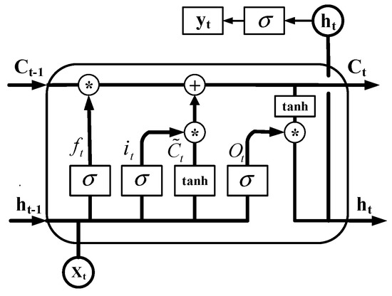
Figure 1.
The structure of the LSTM network.
The LSTM unit receives the current input Xt and the state ht−1 of the tuple and obtains the state Ct−1 of the neuron at time t. We first determine which information to clear through the forget gate, then add new information to the state of the cell through the input gate and update the state of the cell. This process is mainly controlled by the Sigmoid function and the Tanh function to form the neuron state Ct. Finally, the output gate determines which information in the cell is finally output. The memory cell state Ct is calculated by the activation function, and the output gate is dynamically controlled to form the final output ht of the LSTM cell at time t.
According to Figure 1, Equation (3) can be obtained:
where ‘*’ denotes the Hadamard product.
Further considering the weights W and the offsets b of the input, output, and forget gates, Equation (4) can be obtained:
where σ() is the logistic sigmoid function; Wi,x, Wf,x,Wo,x, and WC,x are the four weight matrices applied to the input; and Wi,h, Wf,h, Wo,h, and WC,h are the four weight matrices applied at the previous time step to the output. Additionally, bi, bf, bo, and bC are four bias vectors, and ft, it, and Ot refer to the activation functions of each gate.
Comparing the predicted PV power output and the actual power output, it can be found that the prediction error is irregularly distributed. Based on this fact, BC–LSTM is proposed, which builds an additional model (called the bias compensation network) to predict the prediction bias to minimize the overall prediction error. This method uses the error compensation term to improve the prediction accuracy. The structure of the BC–LSTM network is shown in Figure 2.
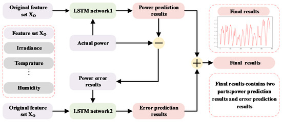
Figure 2.
The structure of BC–LSTM: purple boxes represent input, green boxes represent neural networks, red boxes represent output, and gray boxes represent the features.
3. Performance of the Hybrid Method
The interest in using the framework of the hybrid method is demonstrated in this section, combining the IFFS and the BC–LSTM network for PV forecasting purposes.
The BC–LSTM network uses two LSTM networks to predict the actual PV power and PV power error, respectively. The biggest difference between the hybrid method and traditional BC–LSTM network is that the new feature selection method is used to select feature sets for the prediction network and bias compensation network, respectively. The actual power value and the power error term are generated inconsistently, and the influencing factors are also different. Using the same meteorological data as the model input, its prediction accuracy is poor, and its computational complexity is high. Therefore, a framework for the hybrid method combining the feature selection and BC–LSTM network is proposed, where IFFS is applied to the two LSTM networks to improve prediction accuracy and calculation efficiency. The specific implementation process is shown in Figure 3.
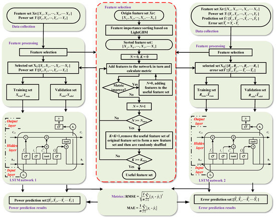
Figure 3.
Flow chart of PV short-term power prediction based on feature optimization method and BC–LSTM network.
Step one: Collect raw data and perform the data processing. The data processing procedure is composed of two sections: data cleaning and data preparation. In the first section, data cleaning includes two aspects: an outlier detector and missing value filling. The original data first uses isolation forests to detect outliers and remove outliers, then uses KNN to fill in the missing values. In the second section, new features are constructed based on the original features.
Step two: Construct the regression model based on LightGBM to obtain the feature importance identification. Then, obtain the optimal feature set according to the algorithm flow in Section 2.1.
Step three: Split the preprocessed data set into training and validation sets. Construct the regression model based on the LSTM network and initialize the parameters. In the tth state of the LSTM, update the cell state based on the input at time t and the state at the previous time t−1. The target at the mth iteration is to update the parameters and minimize the loss function, denoted as follows:
where xi is the ith sample, and yi is the expected result of the ith sample.
Step four: After k iterations, or after the loss function no longer decreases, output the final trained model, LSTM network 1, and the predicted results.
Step five: Subtract the predicted data from the original data to get the error set. The error set and the processed feature set form a new data set. Repeat step two through four for the new data set to get the final trained model, LSTM network 2, and the predicted error results.
Step six: The predicted results in step four and the predicted error results in step five form the final prediction results, and then calculate the metrics.
4. Case Study
4.1. Data Description and Implementation Environment
Two years’ (1 January 2017–31 December 2018) worth of NWP data from the no. 24 PV power plant located in Ningxia Zhongwei, China, were selected for this study. The data resolution is 15 min, and the prediction horizon is one day ahead, with a total of 20-dimensional original features. All data have been preprocessed for performance (the specific operations are shown in Section 3). The features after the data processing procedure are shown in Table 1. To strengthen the results of the generalization ability, the data from 2017 and from January, February, April, May, July, August, October, and November of 2018 are used as the training data set, and the data from March, June, September, and December of 2018 are used as the validation data set. Considering the power generation at sunset is almost zero, the night data is excluded in the training and validation data set. All experiments were run in the python3.6 environment in anaconda, accelerated by NVDIA Geforce RTX2080Ti, CPU Intel(R) Xeon(R) CPU E5-2680 v3@2.50 GHz 2.5 GHz, memory 8 GB.

Table 1.
Data information.
There are three tasks that need to be completed in this case study:
- (1)
- Verify the effectiveness of IFFS.
- (2)
- Verify the superiority of the BC–LSTM network compared to the traditional LSTM network.
- (3)
- Verify the superiority of the hybrid method compared to the BC–LSTM network.
4.2. Feature Selection
4.2.1. Feature Selection Result—LightGBM
According to the ranking results for feature importance in Figure 4, 23 features are selected after excluding {F1, F16, F22, F23, F25, F26} to form a new feature set XI as the comparative feature set.
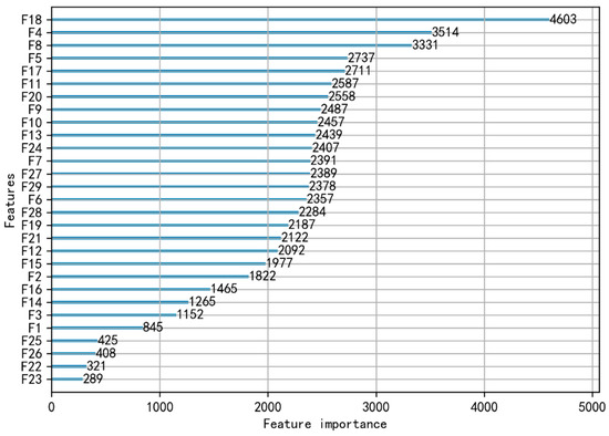
Figure 4.
Feature importance identification results (quantified importance for the 29 meteorological variables, the last six variables being the least important, including {F1, F16, F22, F23, F25, F26}).
4.2.2. Feature Selection Result—IFFS
The features applied to the forecasting model are selected on the basis of feature importance ranking. The evaluation network used is an LSTM network, and the evaluation metric is MAE. After many attempts, when Nmax is 5 and Kmax is 3, the prediction effect is optimal. The specific metric change results are shown in Figure 5.
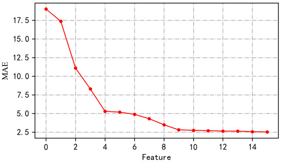
Figure 5.
MAE change chart (according to IFFS, only when the MAE value drops will the MAE and the corresponding feature be recorded).
Sixteen features are selected after excluding {F1, F9, F10, F11, F15, F16, F21, F22, F23, F24, F25, F26, F29} to form a new feature set XS as the optimal feature set.
To illustrate the effectiveness of IFFS, the following three experimental groups are set up for comparative analysis:
- Feature set XO containing 29 original features.
- Feature set XI containing 23 original features selected from the LightGBM feature importance sorting results.
- Feature set XS obtained using IFFS.
4.3. Comparing Different Methods
To solve the three problems mentioned in Section 4.1, the following experimental schemes are designed for comparative analysis:
Scheme (1): The feature set XO is used as an input, and the network uses a standard LSTM network, which will be referred to as the LSTM (XO) network.
Scheme (2): The feature set XI is used as an input, and the network uses a standard LSTM network, which will be referred to as the LSTM (XI) network.
Scheme (3): The feature set XS is used as an input, and the network uses a standard LSTM network, which will be referred to as the LSTM (XS) network.
Scheme (4): The feature set XS is used as the input, and the network uses the BC–LSTM network, which will be referred to as the BC–LSTM (XS) network.
Scheme (5): The feature set XS and the feature set XR are, respectively, used as the inputs of the BC–LSTM networks, which will be referred to as the BC–LSTM (XS + XR) network.
Note: XO, XI, and XS are the feature sets obtained in Section 4.2, where feature set XR is the feature set selected for the error network using IFFS, and the result is XR: {F4, F5, F6, F7, F8, F10, F14, F18, F19, F20, F21, F25, F29}. The evaluation metrics of the five schemes are RMSE, MAE, and R2_adjusted, and the training and verification sets are divided as shown in Section 4.1. RMSE, MAE, and R2_adjusted were defined as follows:
The root-mean-square error (RMSE) measures the difference between the actual values and the forecasting values. It is defined as
The mean absolute error (MAE) is the average of the absolute errors. It is defined as
The adjusted R-square (R2_adjusted) judges whether the predictive model is fitting and reflects whether the prediction deviates from reality, which ranges from [0, 1]. If R2 = 0, the model fits poorly, and if R2 = 1, the model has no errors. However, as the number of independent variables increases, R2 will continue to increase. To eliminate the impact of the number of features, we introduce the R2_adjusted indicator, which is defined as
where N is the number of observations, p is the number of features, yf is the forecast value, ya is the actual value, and ym is the mean value. For fairness of comparison, when the evaluation metrics are RMSE and MAE, all network parameters are optimized by the GridSearch method, as shown in Table 2. When the evaluation metric is training time, the parameter settings of all the networks are the same.
Table 2.
Feature selection result.
- (1)
- The x-axis represents the period, and the y-axis denotes the normalized power values. To better illustrate the comparison of the effects between the different models, the data from different months are selected for display, which is shown in Figure 6.
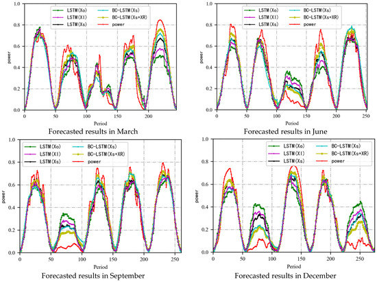 Figure 6. Forecast results: the x-axis represents the period, and the y-axis denotes the normalized power values. The red curve represents the actual power value, and the different curves represent the prediction results of the different models. The best prediction results are given by BC–LSTM (Xs + XR).
 - (2)
- The histogram is used to show the forecast error distribution, and its skewness and variance are calculated, which is shown in Figure 7. The calculation formula is shown as follows:where σx represents the variance of x, E represents expectations, and S(x) represents skewness.
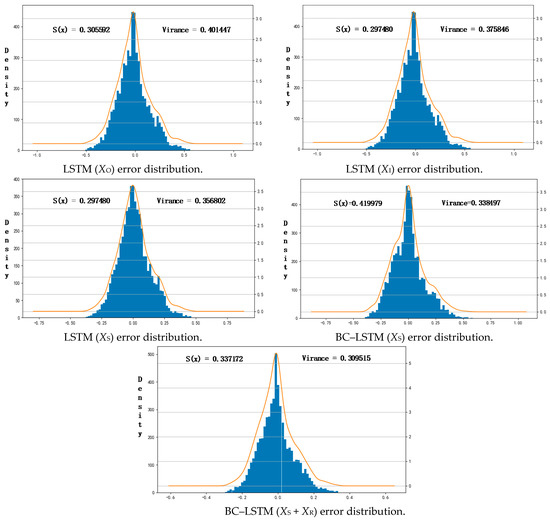 Figure 7. Error distributions: the blue histogram represents the error distribution, and the orange curve fits the error distribution. The smallest variance is given by the BC–LSTM (XS + XR), and the largest deviation is given by the BC–LSTM skewness.
Comparing the experimental results in Figure 6, for dates with relatively stable output power, both LSTM and BC–LSTM networks can achieve satisfactory prediction results. For dates with strong volatility or cloudy days, the BC–LSTM network has stronger prediction capabilities than the traditional LSTM network. For weakly volatile dates, its power has a strong regularity, and its error is small. Therefore, using the bias compensation network to predict its accuracy improvement effect is limited. For dates with large power fluctuations, the difference between the prediction result and the actual power is large. Therefore, constructing a reasonable and effective error network to predict the error value can effectively improve its prediction accuracy, and this is why BC–LSTM performs better than traditional LSTM networks.
In the power system dispatch, the reserve capacity needs to be reduced as much as possible. If the prediction power is greater than the true power, the reserve capacity must be increased; otherwise, some PV power electricity could be abandoned. Therefore, for the same MAE and RMSE, the prediction result with skewness less than 0 is better. It can be seen from Figure 7 that the skewness of the LSTM network is about 0, while the skewness of the BC–LSTM network is less than 0, which means that the BC–LSTM network is more conducive to power system dispatch and reserve capacity reduction.
The evaluation metrics of each experimental group were obtained in Section 4.3. After further analysis of the experimental results (Table 3), the following conclusion can be drawn.
Table 3.
Results.
Comparing the results of Schemes (1)–(3), the results obtained by using IFFS have improved the MAE, RMSE value, and time efficiency. To some extent, this can illustrate the effectiveness of IFFS. Compared with the LightGBM method, IFFS can improve the prediction accuracy by 0.67% and the calculation efficiency by 20%. Comparing feature sets XI and XS, it is not difficult to find that the main difference between feature sets XS and XI is that more feature-forward difference terms are excluded from feature set XS, considering that PV power is mainly related to NWP data, and the forward difference of NWP data is mainly related to power fluctuations. Thus, excluding these features can improve the calculation efficiency and improve the prediction accuracy. This is consistent with the result of IFFS, which, to a certain extent, can further illustrate the effectiveness of IFFS. Moreover, the number of features used in this paper is 29. It is expected that, when the number of features is improved, the improvement effect in terms of time efficiency and accuracy will be higher.
In comparing Schemes (3)–(5), Scheme (4) slightly improves the accuracy compared with Scheme (3) by about 0.27%, but its time efficiency is about half of Scheme (3). Compared with Scheme (3), Scheme (5) takes less time than Scheme (4) to achieve a greater improvement in accuracy. The superiority of BC–LSTM is that it uses two different network structures to predict the power and power error values, respectively, and then obtains the final prediction result. Thus, the accuracy of its prediction result depends on the accuracy of the two networks. Compared with the experimental Scheme (3), Scheme (4) sacrifices a large amount of computational efficiency but only exchanges this for a slight improvement in accuracy. The reason is that the prediction accuracy of the error network is not good. And the experimental results of Schemes (4) and (5) also show that the hybrid method, combining IFFS and the BC–LSTM network, can achieve higher accuracy and computational efficiency compared with the BC–LSTM network without the feature selection.
5. Conclusions
A framework of the hybrid method combining feature selection and the BC–LSTM network is used to perform PV power forecasting. The proposed methods are applied to solve the actual forecast case at the Ningxia Zhongwei no. 24 PV Power Plant in China. Three verification metrics, RMSE, MAE, and training time, are used to evaluate prediction accuracy and calculation efficiency.
The conslusions are summarized as follows:
- (1)
- The optimal feature set for PV power prediction could be selected based on IFFS. Compared with LightGBM, IFFS can improve the prediction accuracy by 0.67% and the calculation efficiency by 20%;
- (2)
- The BC–LSTM network is an effevtive method for predicting fluctuating PV power. Using the same feature set as input, the BC–LSTM performs better than traditional LSTM networks in terms of prediction accuracy by about 0.27%, and the BC–LSTM network is more conducive to power system dispatch and reserve capacity reduction, but it takes more time for training and prediction than the LSTM method.
- (3)
- The hybrid method combining IFFS feature selection and the BC–LSTM network demonstrates significant advantages for PV power prediction, which can achieve improving the prediction accuracy by 0.9% and the calculation efficiency by 10% compared with the BC–LSTM network.
In summary, the hybrid method obtains high-precision prediction results with minimal training time. These results fully demonstrate that the hybrid method has the ability to obtain PV power prediction results with excellent performance for accuracy and calculation efficiency.
There are still many aspects that are worthy of further verification.
- (1)
- In this article, IFFS is applied to a feature selection for PV power prediction, and the prediction accuracy is improved. In the future, more transformation features for PV power prediction could be constructed, and further feature selection could be carried out based on the proposed method.
- (2)
- Positive results have been achieved for PV power prediction based on the proposed hybrid model. The hybrid model could also be applied to the forecast of photovoltaic power plant clusters in the future.
Author Contributions
Conceptualization, C.T. and J.L. (Junjie Lu); methodology, C.T.; software, J.L. (Junjie Lu); validation, J.L. (Jianxun Lang); formal analysis, K.C.; investigation, X.P.; resources, C.T.; data curation, J.L. (Junjie Lu); writing—original draft preparation, J.L. (Junjie Lu); writing—review and editing, C.T.; visualization, J.L. (Jianxun Lang); supervision, S.D.; project administration, C.T.; funding acquisition, C.T. All authors have read and agreed to the published version of the manuscript.
Funding
This work was supported by the National Key R&D Program of China (Technology and application of wind power/photovoltaic power prediction for promoting renewable energy consumption, 2018YFB0904200) and in part by the eponymous Complement S&T Program of State Grid Corporation of China (SGLNDKOOKJJS1800266).
Institutional Review Board Statement
Not applicable.
Informed Consent Statement
Not applicable.
Data Availability Statement
3rd Party Data. Restrictions apply to the availability of these data. Data were obtained from [third party] and are available [from the authors/at URL] with the permission of [third party].
Conflicts of Interest
The authors declare no conflict of interest.
Nomenclature
| XO | Original feature set |
| XI | Original feature set after feature importance sorting |
| XS | Original feature set after feature selection |
| XR | Feature set selected for error network using feature selection method |
| Y | Historical power set |
| m | Number of feature input |
| d | Number of hidden layer nodes |
| e | Number of hidden layer |
| η | Decayed learning rate parameter: initial learning rate |
| ηmin | Decayed learning rate parameter: minimum of learning rate |
| dr | Decayed learning rate parameter: decay rate |
| ds | Decayed learning rate parameter: decay steps |
| dp | Dropout parameter: dropout rate |
| bs | Mini-batch parameter: batch size |
| Es | EarlyStopping rounds |
| Ep | Mini-batch parameter: epochs of training |
| NWP | Numeric Weather Prediction |
| tanh | Activation function of tanh |
| σ(x) | Activation function of sigmoid |
| ht | Output of the hidden layer |
| ft | Forget gates in the t-th period |
| it | Input gates in the t-th period |
| Ct | Neuron states in the t-th period |
| W | Weight matrix |
| b | Bias vector |
| GBDT | Gradient Boosting Decision Tree |
| Kmax | Threshold of feature selection |
| Nmax | Threshold of feature selection |
| RNN | Recurrent Neural Network |
| LSTM | Long Short-Term Memory Network |
| BC–LSTM | Bias Compensation–Long Short-Term Memory Network |
| CNN | Convolutional Neural Network |
| IFFS | Improved Forward Feature Selection |
| MAE | Mean absolute error |
| RMSE | Root-mean-square error |
References
- Chai, M.; Xia, F.; Hao, S.; Peng, D.; Cui, C.; Liu, W. PV power prediction based on LSTM with adaptive hyperparameter adjustment. IEEE Access 2019, 7, 115473–115486. [Google Scholar] [CrossRef]
- Sobri, S.; Koohi-Kamali, S.; Rahim, N.A. Solar photovoltaic generation forecasting methods: A review. Energy Convers. Manag. 2018, 156, 459–497. [Google Scholar] [CrossRef]
- Akhter, N.M.; Mekhilef, S.; Mokhlis, H.; Shah, N.M. Review on forecasting of photovoltaic power generation based on machine learning and metaheuristic techniques. IET Renew. Power Gener. 2019. [Google Scholar] [CrossRef]
- Wan, C.; Zhao, J.; Song, Y.; Xu, Z.; Lin, J.; Hu, Z. Photovoltaic and solar power forecasting for smart grid energy management. CSEE J. Power Energy Syst. 2015, 1, 38–46. [Google Scholar] [CrossRef]
- Wang, F.; Zhen, Z.; Mi, Z.; Sun, H.; Su, S.; Yang, G. Solar irradiance feature extraction and support vector machines based weather status pattern recognition model for short-term photovoltaic power forecasting. Energy Build. 2015, 86, 427–438. [Google Scholar] [CrossRef]
- Wang, F.; Zhen, Z.; Liu, C.; Mi, Z.; Hodge, B.-M.; Shafie-khah, M.; Catalão, J.P.S. Image phase shift invariance based cloud motion displacement vector calculation method for ultra-short-term solar PV power forecasting. Energy Convers. Manag. 2018, 157, 123–135. [Google Scholar] [CrossRef]
- Wang, F.; Zhang, Z.; Chai, H.; Yu, Y.; Lu, X.; Wang, T.; Lin, Y. Deep Learning Based Irradiance Mapping Model for Solar PV Power Forecasting Using Sky Image. IEEE Ind. Appl. Soc. Annu. Meet. 2019, 1–9. [Google Scholar] [CrossRef]
- Tang, J.; Lv, Z.; Zhang, Y.; Yu, N.; Wei, W. An improved cloud recognition and classification method for photovoltaic power prediction based on total-sky-images. J. Eng. 2019, 18, 4922–4926. [Google Scholar] [CrossRef]
- Massucco, S.; Mosaico, G.; Saviozzi, M.; Silvestro, F. A hybrid technique for day-ahead PV generation forecasting using clear-sky models or ensemble of artificial neural networks according to a decision tree approach. Energies 2019, 12, 1298. [Google Scholar] [CrossRef]
- Wang, F.; Pang, S.; Zhen, Z.; Li, K.; Ren, H.; Shafie-Khah, M.; Catalão, J.P.S. Pattern Classification and PSO Optimal Weights Based Sky Images Cloud Motion Speed Calculation Method for Solar PV Power Forecasting. In Proceedings of the 2018 IEEE Industry Applications Society Annual Meeting (IAS), Portland, OR, USA, 23–27 September 2018. [Google Scholar] [CrossRef]
- Sun, Y.; Wang, F.; Mi, Z.; Sun, H.; Liu, C.; Wang, B.; Lu, J.; Zhen, Z.; Li, K. Short-term prediction model of module temperature for photovoltaic power forecasting based on support vector machine. In Proceedings of the International Conference on Renewable Power Generation (RPG 2015), Beijing, China, 17–18 October 2015. [Google Scholar] [CrossRef]
- Pierro, M.; Bucci, F.; De Felice, M.; Maggioni, E.; Moser, D.; Perotto, A.; Spada, F.; Cornaro, C. Multi-Model Ensemble for day ahead prediction of photovoltaic power generation. Sol. Energy 2016, 134, 132–146. [Google Scholar] [CrossRef]
- Massidda, L.; Marrocu, M. Use of Multilinear Adaptive Regression Splines and numerical weather prediction to forecast the power output of a PV plant in Borkum, Germany. Sol. Energy 2017, 146, 141–149. [Google Scholar] [CrossRef]
- Zhou, H.; Zhang, Y.; Yang, L.; Liu, Q.; Yan, K.; Du, Y. Short-Term Photovoltaic Power Forecasting Based on Long Short-Term Memory Neural Network and Attention Mechanism. IEEE Access 2019, 7, 78063–78074. [Google Scholar] [CrossRef]
- Zang, H.; Cheng, L.; Ding, T.; Cheung, K.W.; Liang, Z.; Wei, Z.; Sun, G. Hybrid method for short-term photovoltaic power forecasting based on deep convolutional neural network. IET Gener. Transm. Distrib. 2018, 12, 4557–4567. [Google Scholar] [CrossRef]
- Wang, H.; Liu, Y.; Zhou, B.; Li, C.; Cao, G.; Voropai, N.; Barakhtenko, E. Taxonomy research of artificial intelligence for deterministic solar power forecasting. Energy Convers. Manag. 2020, 214, 12909. [Google Scholar] [CrossRef]
- Rana, M.; Koprinska, I.; Agelidis, V.G. Univariate and multivariate methods for very short-term solar photovoltaic power forecasting. Energy Convers. Manag. 2016, 121, 380–390. [Google Scholar] [CrossRef]
- Yuan, X.; Li, L.; Shardt, Y.; Wang, Y.; Yang, C. Deep learning with spatiotemporal attention-based LSTM for industrial soft sensor model development. IEEE Trans. Ind. Electron. 2020. [Google Scholar] [CrossRef]
- Rana, M.; Rahman, A. Multiple steps ahead solar photovoltaic power forecasting based on univariate machine learning models and data re-sampling. Sustain. Energy Grids Netw. 2020, 21, 100286. [Google Scholar] [CrossRef]
- Yu, D.; Lee, S.; Lee, S.; Choi, W.; Liu, L. Forecasting Photovoltaic Power Generation Using Satellite Images. Energies 2020, 13, 6603. [Google Scholar] [CrossRef]
- Jiang, Y.; Yang, Y.; Wu, Q.; Chi, X.; Miao, J. Research on Predicting the Short-term Output of Photovoltaic (PV) Based on Extreme Learning Machine Model and Improved Similar Day. In Proceedings of the 2019 Innovative Smart Grid Technologies Asia (ISGT Asia), Chengdu, China, 21–24 May 2019. [Google Scholar] [CrossRef]
- Eseye, A.T.; Lehtonen, M.; Tukia, T.; Uimonen, S.; Millar, R.J. Adaptive Predictor Subset Selection Strategy for Enhanced Forecasting of Distributed PV Power Generation. IEEE Access 2019, 7, 90652–90665. [Google Scholar] [CrossRef]
- Eseye, A.T.; Zhang, J.; Zheng, D. Short-term photovoltaic solar power forecasting using a hybrid Wavelet-PSO-SVM model based on SCADA and Meteorological information. Renew. Energy 2018, 118, 357–367. [Google Scholar] [CrossRef]
- Zang, H.; Cheng, L.; Ding, T.; Cheung, K.W.; Wei, Z.; Sun, G. Day-ahead photovoltaic power forecasting approach based on deep convolutional neural networks and meta learning. Int. J. Electr. Power Energy Syst. 2020, 118, 105790. [Google Scholar] [CrossRef]
- Behera, M.K.; Majumder, I.; Nayak, N. Solar photovoltaic power forecasting using optimized modified extreme learning machine technique. Eng. Sci. Technol. Int. J. 2018, 21, 428–438. [Google Scholar] [CrossRef]
- Wang, K.; Qi, X.; Liu, H. A comparison of day-ahead photovoltaic power forecasting models based on deep learning neural network. Appl. Energy 2019, 251, 13315. [Google Scholar] [CrossRef]
- Behera, M.K.; Nayak, N. A comparative study on short-term PV power forecasting using decomposition based optimized extreme learning machine algorithm. Eng. Sci. Technol. Int. J. 2019. [Google Scholar] [CrossRef]
- VanDeventer, W.; Jamei, E.; Thirunavukkarasu, G.S.; Seyedmahmoudian, M.; Soon, T.K.; Horan, B.; Mekhilef, S.; Stojcevski, A. Short-term PV power forecasting using hybrid GASVM technique. Renew. Energy 2019, 140, 367–379. [Google Scholar] [CrossRef]
- Aprillia, H.; Yang, H.T.; Huang, C.M. Short-Term Photovoltaic Power Forecasting Using a Convolutional Neural Network–Salp Swarm Algorithm. Energies 2020, 13, 1879. [Google Scholar] [CrossRef]
- Ahn, H.K.; Park, N. Deep RNN-Based Photovoltaic Power Short-Term Forecast Using Power IoT Sensors. Energies 2021, 14, 436. [Google Scholar] [CrossRef]
- Wang, K.; Qi, X.; Liu, H. Photovoltaic power forecasting based LSTM-Convolutional Network. Energies 2019, 189, 116225. [Google Scholar] [CrossRef]
- Mao, M.; Cao, Y.; Chang, L. Improved fast short-term wind power prediction model based on superposition of predicted error. In Proceedings of the 2013 4th IEEE International Symposium on Power Electronics for Distributed Generation Systems (PEDG), Rogers, AR, USA, 8–11 July 2013; p. 116225. [Google Scholar] [CrossRef]
- Ke, G.; Meng, Q.; Finley, T.; Wang, T.; Chen, W.; Ma, W.; Ye, Q.; Liu, T.-Y. Lightgbm: A highly efficient gradient boosting decision tree. Adv. Neural Inf. Process. Syst. 2017, 3146–3154. [Google Scholar] [CrossRef]
- Hochreiter, S.; Schmidhuber, J. Long short-term memory. Neural Comput. 1997, 9, 1735–1780. [Google Scholar] [CrossRef]


Publisher’s Note: MDPI stays neutral with regard to jurisdictional claims in published maps and institutional affiliations. |
© 2021 by the authors. Licensee MDPI, Basel, Switzerland. This article is an open access article distributed under the terms and conditions of the Creative Commons Attribution (CC BY) license (https://creativecommons.org/licenses/by/4.0/).