
On the Verification of the Pedestrian Evacuation Model †


1
Faculty of Science, Jan Evangelista Purkyně University, České Mládeže 8, 400 96 Ústí nad Labem, Czech Republic
2
Faculty of Mathematics and Physics, Charles University Prague, Sokolovská 83, 186 75 Praha, Czech Republic
*
Author to whom correspondence should be addressed.
†
The research was supported by the grant No. UJEP-IGA-TC-2019-53-02-2 of IGA UJEP. The authors
acknowledge this support.
‡
These authors contributed equally to this work.
Mathematics 2021, 9(13), 1525; https://doi.org/10.3390/math9131525
Submission received: 1 June 2021
/
Revised: 24 June 2021
/
Accepted: 25 June 2021
/
Published: 29 June 2021
(This article belongs to the Section Mathematics and Computer Science)
Abstract
:In this article we deal with numerical solution of macroscopic models of pedestrian movement. From a macroscopic point of view, pedestrian movement can be described by a system of first order hyperbolic equations similar to 2D compressible inviscid flow. For the Pedestrian Flow Equations (PFEs) the density and the velocity are considered as the unknown variables. In PFEs, the social force is also taken into account, which replaces the outer volume force term used in the fluid flow formulation, e.g., the pedestrian movement is influenced by the proximity of other pedestrians. To be concrete, the desired direction of the pedestrian movement is density dependent and is incorporated in the source term. The system of fluid dynamics equations is thus coupled with the equation for . The main message of this paper is the verification of this model. Firstly, we propose two approaches for the source term discretization. Secondly, we propose two splitting schemes for the numerical solution of the coupled system. This leads us to four different numerical methods for the PFEs. The novelty of this work is the comparative study of the numerical solutions, which shows, that all proposed methods are in the good agreement.
1. Introduction
Modeling of the movement of pedestrians is an interesting non-linear complex problem, where physical and environmental conditions (e.g., visibility see [1]), as well as social and psychological conditions (e.g., fatigue, see [2]), manifest themselves. The complexity of the dynamics of pedestrian movement is illustrated by the emergence of collective effects and self-organisation phenomena. One of the most important practical applications of these models is the ability to simulate the movement of a crowd in panic situations, such as floods, fires, etc. In such cases, it is necessary to have evacuation plans in place and try to predict people’s behavior.
In general, there are two classes of the pedestrian behaviour models, macroscopic and microscopic. We are mainly interested in the macroscopic approach where pedestrians are considered as a continuum and their behaviour is described by two-dimensional fluid dynamics equations for an inviscid adiabatic flow subject to outer volume forces. This approach was proposed in [3].
The outer volume forces represent a relaxation term towards a desired velocity. Since the model is devised for room or open space evacuation situations, the desired pedestrian velocity depends on the density distribution. The pedestrians want to avoid the regions with high densities, so the magnitude of the desired velocity is a decreasing function of the density. Such a function stems from the experimental investigations of pedestrian evacuation problems. For various definitions of density dependent magnitude of desired velocity see [4,5,6]. A detailed overview can be found in [7]. Also the desired direction of pedestrian velocity is density dependent. The desired direction of a pedestrian motion is given as a unit tangential vector to the fastest path to the exit. This works like a car navigation system. The pedestrian knows the magnitude of the velocity in which he would like to go and seek the fastest path to exit. Instead of seeking the fastest path, the so called Eikonal equation can be used for the determination of the desired direction of pedestrian velocity. See [8] for the detailed explanation. The above described model falls into the class of macroscopic models, where the state of the system is described by locally averaged quantities. It was originally proposed in [9] as an extension of the vehicular traffic models described in [10,11]. More models originated from different pedestrian behaviour and strategies are proposed and analyzed in [7]. The reader will find a classification of macroscopic models, and some qualitative properties such as hyperbolicity are further studied. The model of pedestrian with disctinct desired direction is studied in [12], here the two-phase pedestrian flow model is taken into account.
In the microscopic approach, the pedestrian is considered as an individual interacting with others pedestrians. Example of this approach is the model, where the pedestrians are described by the system of N ordinary differential equations (ODE), here N stands for the number of pedestrians. This model is studied in [13]. Here are stated simulations of the high-density crowd behaviour in the real world objects and situations such as sporting events and pilgrimage places. The transition from microscopic (ODE) to macroscopic model is listed in [14]. Reader founds deep compilation of the literature devoted to booth approaches in [3]. Here is stated more detailed description and differentiation of microscopic models such as a social force model, cellular automata models (CA) or gradient flow methods (macroscopic approach). The comparison of the cellular automata model with the PFEs (macroscopic) can be found in [15], where the new Cellular Automaton (CA) model is proposed for the simulation of the pedestrian flow and the comparative study is presented. The level between microscopic and macroscopic scale is represented by the mesoscopic scale. An example of this kind of models is kinetic model described in [16].
It is seen from a review of the literature that extensive research is currently underway on modelling pedestrian evacuation and related situations. In this paper, we are interested in a model that is based on fluid dynamics equations and formulated as a hyperbolic system with a source term on the right hand side of the equation. In accordance with [17], such a system is usually solved by the splitting method. Because there is a lack of experimental data from real-life situations in this case, it is difficult to validate that the numerical results correspond to real-world situations. But what is possible is to study whether the numerical solution is correct.
To this end, we have proposed two substantially different numerical methods of splitting: Splitting Scheme I and Splitting scheme II. The paper emphasizes which parts of discretization using the Finite Volume Method (FVM) and the combined Finite Volume and the Discontinuous Galerkin method (FV-DG), are original. The choice of the numerical flux in both methods is original (the original numerical flux of the Vijayasundaram type, the method of solving the Eikonal equation using Dijkstra’s algorithm for the shortest path in the graph is original). The proposed numerical methods are mutually compared. A representative sample of adequate problems from pedestrian evacuation is solved. The novelty of the paper is a comparison of the results of different numerical methods for solving the given problem. The article thus deviates from the usual scheme One problem-One method-One result. We have One problem-Four methods-Four results relatively in a good agreement. The choice of method is then up to the user: simplicity versus higher order versus computational time.
The paper is organized as follows. In Section 2 the macroscopic model of pedestrian flow describing the room or open space pedestrian evacuation is formulated. The splitting technique and its numerical realization is explained in Section 3. The physically relevant computations of various evacuation scenarios are presented in Section 4. A conclusion summarizing the results achieved and emphasizing the novelty of the paper is included in Section 5.
2. Governing Equations
Let us consider the pedestrian flow in the polygonal domain and time interval with . We suppose that the boundary , where the subscript w states for wall and o for the exit (outflow). The bar in denotes the closure of the set . We further suppose that the subsets are disjoint and formed by a finite number of connected sets, open with respect to the topology on , where the one-dimensional measure meas, i.e., is not a point. Such a setting is convenient for the modeling of pedestrian evacuation problems in order to predict the pedestrian behavior in panic situations. The system of the PDE’s for the vector valued function is
Here the unknown variable forms a vector . We denote by the density of pedestrians in [ped/m] and by their velocity in [m/s].
The fluxes are defined by
The power law for isentropic gases expressing the dependence of the pressure p on the density is used in the definition of the fluxes . In our computations the constant is set and the Poisson constant . The source term is given by
Here V represents the magnitude of the desired velocity in which the pedestrian would like to go, we suppose . The notation means that and . The definition of can be found in [3]. In our work we use the exponential dependence
where , the maximum density at which is hardly possible to move is set and the speed of free flow . These parameters setting is based on [4], where experimental investigation of pedestrian behavior is listed.
The unit vector is the preferred direction of the movement of pedestrians, , and it depends on the distribution of the density in the whole domain , which we express by the functional dependence
The function V and the unit vector characterize how the speed of pedestrians changes with the density. The parameter represents a relaxation time describing how fast pedestrians correct their current velocity to the desired one . We set this parametr according to the validation of the model with experimental pedestrian movement.
2.1. Functional Dependence
To determine the direction (desired velocity direction) we have basically two equivalent possibilities how to define functional in (4).
2.1.1. Integral Formulation
The numerical approximation of in (6) is obtained via Dijkstra’s algorithm, see original paper [18] or more detailed explanation in [19], and thus we denote it by the subscript D In (6) the minimum is taken over all piecewise regular curves in , parametrized by the parameter with the property . Let us note that the whole distribution of the density at each time instant t has to be given to determine .
2.1.2. Differential Formulation
Equation (8) is the so called Eikonal equation of pedestrian flow problem. This equation is completed by the boundary condition (9). The numerical approximation of in (8) and (9) is obtained via the Bornemann-Rasch algorithm, see [20], and thus we denote it by the subscript .
An alternative approach how to define the functional was introduced in [21]. The physical meaning of as the tangential vector to fastest path to the exit and as the shortest time to reach the exit for a given magnitude of velocity V is explained in [8,21].
The boundary condition is prescribed
where B is appropriate boundary operator. For the boundary condition on the wall we use a normal component of velocity equal to zero
On the exits we prescribe , the space behind the exit is free and empty and pedestrians can leave this space. The more detailed specification of the boundary conditions is described in [8]. Let us note that due to the hyperbolicity of the system the Dirichlet boundary condition cannot be prescribed directly. We solve a linearized initial-boundary value problem instead.
3. Numerical Solution
The usual way how to solve the hyperbolic systems with the source term is the splitting technique.
3.1. Splitting Schemes
We consider two splitting schemes for system (1). Since there are various possibilities of the splitting, a question arises, if the equations are solved “right”. This is related to the notion of “verifiation of the model”. We answer this question from the numerical point of view. In what follows, we discretize parts of the continuum model by substantially different numerical techniques. Finally we show that the numerical results obtained by the different numerical methods are in a good agreement.
3.1.1. Splitting Scheme I
3.1.2. Splitting Scheme II
Remember that the first component of has the physical meaning of density, .
Above stated splitting Schemes (12)–(14) (Splitting Scheme I) and (15) and (16) (Splitting Scheme II) are employed to numerically solve system (1). Booth schemes are applied in an iterative manner. We employ Finite Volume Method (FV) for the discretization (12)–(14), see Section 3.2, while Finite Volume Method in space and the Discontinuous Galerkin Method in time are used for (15) and (16) (FV-DG), see Section 3.5.
In booth schemes we use triangular mesh , where is an index set and . Closed triangles , have usual properties from the finite element method. By the discretization a partition of the time interval is meant. We denote by the size of time step between and and . We denote the set of all vertices of the triangulation by and the set of all edges of by .
3.2. FV Discretization of the Splitting Scheme I
Since we employ the Finite Volume Method in the Spliting scheme I, the approximate solution is considered as piecewise constant in at the time instant
Further we denote
and derive the FV scheme for .
3.2.1. FV Discretization of the Hyperbolic System (12)
Let us assume that is the exact solution of (12). We integrate (12) over , exchange the integration and partial differentiation in the first term and use the Green’s theorem with respect to the space coordinates. Then
Writing , , where is an index set of neighboring triangles to (special treatment has to be done if has a side on ) and approximating
where is the area of and is the so called numerical flux, we derive from (18) the semi-discrete approximation of the hyperbolic system (12)
Here is the length of the side . We use the original numerical flux of Vijayasundaram type proposed in [22]. Its brief description can be found in [8].
For having a side on the boundary , the boundary conditions have to be taken into account. On the walls we use inviscid mirror boundary conditions from ([23], p. 415). Boundary conditions on exit are obtained from solution of a linearized 1D Riemann problem. The formulas for boundary conditions can be found in [8].
If we take Equation (21) for all , we get the vector form of the semi-discrete approximation of (12)
where
Equation (22) is equipped with the initial condition
where is defined in (10). We denote the approximate solution of (22) at time instant by , i.e.,
The following second order Runge–Kutta method can be used for the discretization of Equation (22)
where
Another possibility is to use the Euler method for the discretization of Equation (22)
The initial condition is set according to (25)
3.2.2. FV Approximation of in (13)
The numerical approximation of will be sought in the space of piecewise constant functions on at , i.e.,
3.2.3. FV Approximation of
To compute integral in (6) we approximate at vertex by . The approximation is obtained by the minimization process over edges of the triangulation only. To this end we approximate the quantity on each edge by a arithmetic mean of , at vertices , of the edge E, see (32). The approximations of point values of are obtained from the piecewise constant approximations of on triangles as weighted averages of values on the set of triangles having the point P in common. The definition of V and relation (3) is taking into account. Let us note that the first component of is the approximation of the density. Assuming above mentioned leads the integral in (6) can be determined exactly. The meaning of this integral is the time it takes to go from the vertex P to the exit . The pedestrian path is formed by edges E of the graph given by the triangulation and we get
Here represents the euclidean norm (length) of the edge E, is the shortest path in the graph starting from the vertex P and ending in some vertex of . Since we can define norm of an edge E
the term shortest path means with respect to this norm. According to the physical meaning of quantities in the definiton (33) the shortest means the fastest.
The problem of finding shortest path is solved by modified Dijkstra’s algorithm where we use norm (33) instead of the length of the edge E. We utilize the fact the graph is not oriented and choose the starting vertex as the vertex of the boundary and set the ending vertex . In [24] the multiple starting point Dijkstra’s algorithm has been proposed. This algorithm computes the approximations for all vertices in one run taking an arbitrary vertex lying on as the starting point. The more detailed description can be found in [8].
From point values , , the piecewise linear approximation of in the space
is constructed. The approximation of in (5) on at the time is defined
and used for the approximation of in (31)
For the simplicity of notation the argument in is written as although depends only on the piecewise constant approximation of the density. Relation (34) expresses the fact that depends on the approximation of the density on all .
3.2.4. FV Approximation of
We implemented the Bornemann and Rasch algorithm [20] for the solution of the Eikonal Equations (8) and (9). The function (called potential) is approximated by the piecewise linear function . The key point of this algorithm is the use of the Hopf-Lax formula in order to obtain the piecewise linear finite element solution of the certain local Dirichlet problem. To this end we construct the approximations of point values of from the piecewise constant approximations of on triangles as weighted averages of values on the set of triangles having the point P in common.
The sought potential is the fix point of the operator , where is the so called Hopf-Lax update function:
Here is the boundary of the set of volumes having the vertex P in common. The details about the minimization process in Hopf-Lax update Formula (35) and the convergence of the fix point iterations
can be found in [20]. Having computed the potential at each vertex of the mesh, we assess the gradient at the centre of gravity of the triangle and the quantity
is used for the approximation of in (31)
3.3. Discretization of System (14)
Integrating (14) over , we proceed analogously as in the case of the discretization of the hyperbolic system (12). We define the semi-discrete approximation of (14) as
The notation (19), (23) and (26) and the analogous notation for and the source term
is used. The quantity is obtained from using the relations (34) or (37). Equation (38) can be solved numerically by the same Runge–Kutta method as Equation (22).
where
Another possibility is to use the Euler method for the discretization of Equation (38)
3.4. Splitting Algorithm I
The numerical solution of the Splitting Scheme I is numerically performed by the following Algorithms 1 and 2:
| Algorithm 1 Runge-Kutta splitting |
| Set the initial condition and the method M for the determination of direction , , fordo (1) ; ; (2) ; (3) ; ; ; end for |
In (1) the following notation is used
In (3) the following notation is used
If the Euler method (29) and (46) is used for the numerical solution of (22) and (38), respectively, then steps (1) to (3) are replaced by
| Algorithm 2 Euler splitting |
| fordo (1) ; (2) ; (3) ; end for |
Definition 1.
We say that the piecewise constant vector valued function , defined almost everywhere in the computational domain Ω, is the finite volume solution of (12)–(14), if for all , where is the interior of , i.e., , and are obtained from the Splitting Algorithm I as components of . The function is the approximate solution at time on the triangulation . The vector is the value of the approximate solution on the finite volume at time .
3.5. FV-DG Discretization of the Splitting Scheme II
The FV-DG space-time discontinuous Galerkin method was derived in [8]. In the following paragraphs we briefly summarize it. Let q be an integer and the space of polynomials of degree l on for . The approximate solution is sought in the finite element space
The approximate solution can be written in the form
Provided is a function defined in , we use the notation
if the one-sided limits exist. We put , where is the piecewise constant projection of the initial condition on the mesh .
3.6. FV-DG Approximation of in (15)
The desired direction in (15) depends on the distribution of . Two formulations of the functional are considered in (15), namely and defined in (5)–(9). The meaning of subscripts is the same as above.
We denote the approximation as . This approximation is computed from values , precisely from the density component of value .
3.6.1. FV-DG Approximation of
Assume in the given time instant we have the piecewise constant density , for m = 1 we have initial condition. We construct a continuous piecewise linear recovery from and determine the approximations of velocity V given by (3) for all vertices
Having point values the situation is similar to the Section 3.2.3 and with the same notation the approximation of is defined
To find the shortest path in the graph given by the triangulation the modified Dijkstra’s algorithm is employed. From the values , the piecewise linear function is constructed. This recovery is used to compute gradients of on triangles . The point approximations of by weighted average of gradients of is determined
where is the set of triangles from having the vertex P in common and weights in (52) are areas of each triangle .
3.6.2. FV-DG Approximation of
3.6.3. FV-DG Approximation of the Direction
Having approximate point values of , for each of the above mentioned approaches, the approximation on is constructed. Firstly we define the piecewise linear function on . Secondly this function is extended on to be constant and the approximation is set
The passage from to the definition (54) can be written as
where the functionals and represent the process described above, see Section 3.6.1 and Section 3.6.3. Here denotes the restriction . The upper index of indicates that is computed from values , although is defined on .
3.7. FV-DG Discretization of (16)
The discretization of (16) is described in detail in [8]. Here we mention the main ideas. Let be the exact solution of (1). Multiplying (1) by and integrating over , using the Green’s theorem with respect to the space coordinates and taking sum over all elements we obtain (some manipulation needed and using the fact is constant with respect to the space)
where by we denoted .
Firstly we discretize the time derivative. Detailed procedure for the treatment of the time derivative can be found in [8]. This procedure is based on the integration by parts. The result of this is the following identity
where we use the notation introduced in (49) and .
Secondly, the integral over in (56) is approximated. We use the numerical flux
where and denote the values of on considered from the interior and exterior of , respectively.
The same numerical flux as in (12) is used including the boundary conditions specification.
3.8. Resulting FV-DG Scheme
Using both key ingredients, time derivative and numerical flux together with treatment of the boundary condition for each time interval , we define the following form
where denotes the part of the boundary of lying in the interior of , denotes the part of the boundary of lying on and is given by the boundary conditions.
Definition 2.
If we consider are the basis functions of , the relation (60) for each is a system of nonlinear algebraic equations. The number of equations is equal , here is the number of triangles. The system (60) is solved for each time level . For this task we use a Newton-like method for the numerical solution of the compressible Euler equations, cf. ([23] Chapter 8).
Solution of FV-DG Scheme
As the result of the used numerical flux of Vijayasundaram type, we can linearize the form given by (59) as
where the form is linear with respect to its third argument. The formula for contains the linearized numerical flux and together with can be found in [8].
Taking into account (48), we write system (60) as
which is system of algebraic equations (for each ). Using linearization (61) we approximate by the following sequence of approximations
where solves
4. Results
We present the comparative study of the proposed Splitting schemes I and II from the numerical point of view. The described methods are compared on domains with different geometries. Several meshes grading from coarse to fine are used. Let us stress that we have tested two different numerical methods on the representative sample of computational domains. Moreover, the software for the Finite Volume Method was written by P. Kubera (the first author), while the software for the Discontinuous Galerkin Method was written by V. Dolejší and it was used as the black box with his permission. The detailed description of Dolejší’s method can be found in [8] and generally in [23]. In each splitting scheme I and II the two different approaches for the determination of , namely Bornemann-Rasch and Dijkstra’s algorithms, were used. So we gained a more general insight on the behavior of different methods for pedestrian movement. See also the further comparison with the new Cellular Automaton model proposed recently by the authors in [15].
Quantities we are interested in are the distribution of the density (the dimension being pedestrian per square meter in the distinction of the fluid dynamics density in kg/m) over the domain and the evacuation time in seconds , i.e., the time when the domain is considered to be empty of any people. See the first paragraph in Section 3 for the details how the results have been computed. For each of test cases we use two methods for the determination of in (4). For the numerical solution of in the integral Formulation (6) the abbreviation DA is used and it suggests the Dijkstra’s algorithm. For the numerical solution of in the differential Formulation (8) the abbreviation BR indicates the Bornemann-Rasch algorithm.
Let us define the quantity
giving the number of pedestrians in the domain at the time instant . The quantity is approximated numerically using the computed piecewise constant approximation of the density at time . We consider the domain to be empty if the quantity , where is a prescribed number. We set for all methods.
The parameters of the model are listed below. In the power law for isentropic gases we set , (See the definition of fluxes in (1)). Further we set , , in (3) and in the source term in (1). We use our original numerical flux of Vijayasundaram type in (24) and (59), for its definition see [8,22].
4.1. Domain with One Obstacle
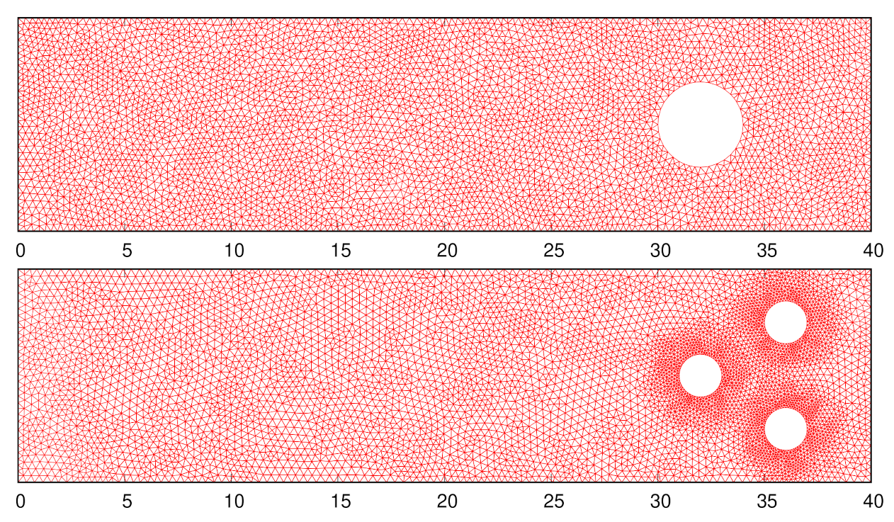
The first example is the evacuation of the rectangular domain 40 × 10 m with one circular obstacle, see Figure 1 (top). The outflow is assumed on the entire vertical right hand side. The wall boundary is assumed elsewhere. This can simulate the open space amphitheatre with a stage in the case when the people are running out of the amphitheatre through a broken wall denoted as the outflow . Initial condition was set
The results concerning the evacuation time are summarized in Table 1. We see that the difference in is less than two seconds.
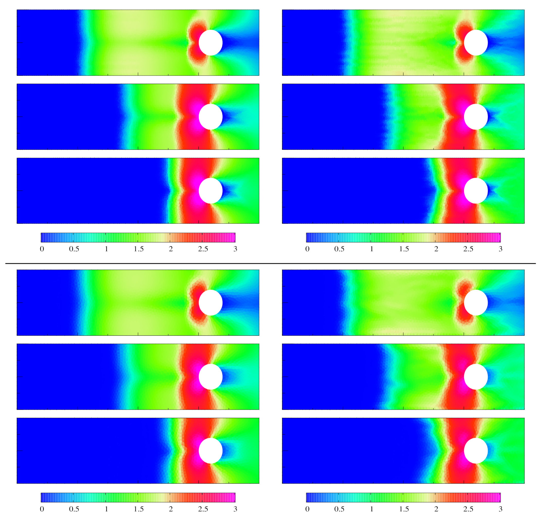
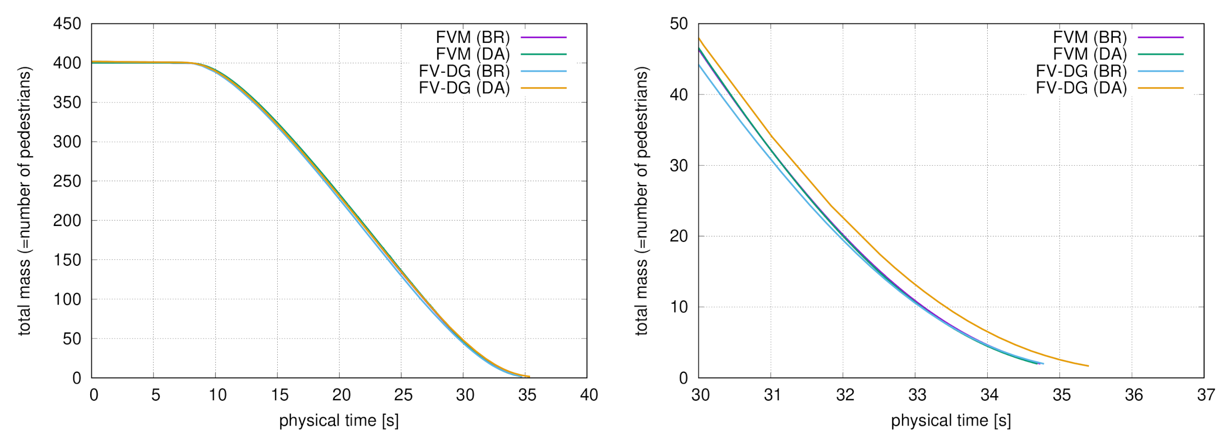
In Figure 2, the evolution in time s of the pedestrian density is drawn. The intuitive movement of pedestrians towards the right hand side can be observed. In each row of figures, the FV and the FV-DG methods are compared. We see all methods are in a good agreement. In Figure 3 the time evolution of the total number of pedestrians is shown.
4.2. Domain with Three Obstacles
Here we present results for the simulation of the evacuation of the rectangular domain 40 × 10 m with three circular obstacles, see Figure 1 (bottom). We suppose boundary and initial conditions and also parameters of the model to be the same as for one circular obstacle above.
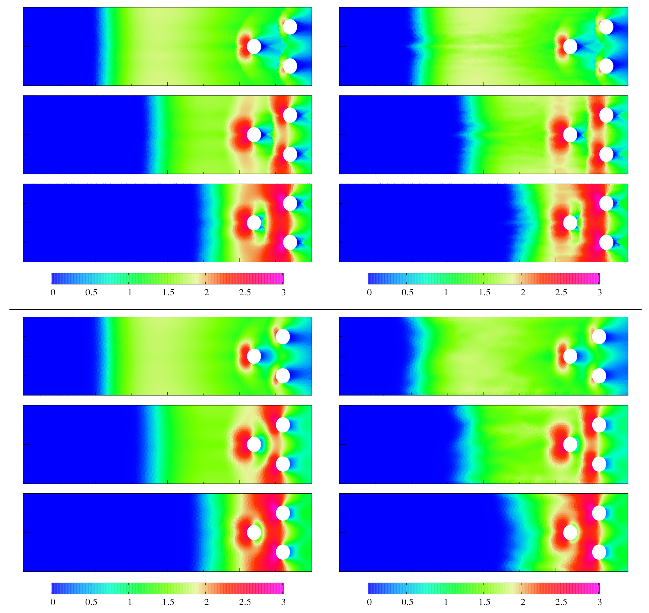
Computational results are shown in Table 2. We can see the difference in being smaller than one second for all methods on all tested meshes. The evolution of the pedestrian density in time is depicted in Figure 4. The intuitive behaviour with the high-density domain in front of the obstacles can be seen for all methods. The dependence of the total number of pedestrians for all tested methods is shown in Figure 5. The curves almost coincide (left). The small difference can be seen on the close view (right). We see that all methods are in a good agreement.
4.3. H-Shape Domain Evacuation
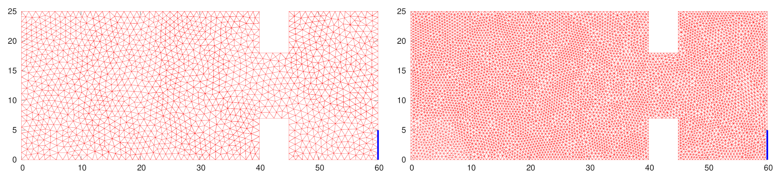
Further we present an evacuation through a narrowing followed by an empty space with the non-symmetric exit, see Figure 6. The so-called H-shape domain represents an example of the non-convex domain. The convexity of the domain does not play any role in the design of the proposed numerical methods. The geometry is defined
The outflow boundary condition is prescribed on
and the wall boundary condition on . We prescribe the initial condition
Table 3 shows the computational results obtained by the FV and by the FV-DG methods. See the description of table, the use of the DA or BR algorithm in the pedestrian flow model (both FV and FV-DG) causes more significant differences in the evacuation time . On the other hand the FV and FV-DG model with the same type of the computation of the desired direction of motion (i.e., DA or BR) produce the and being in a good agreement. The dependence of the pedestrian evacuation model on the use of the DA or BR algorithms has to be further studied.
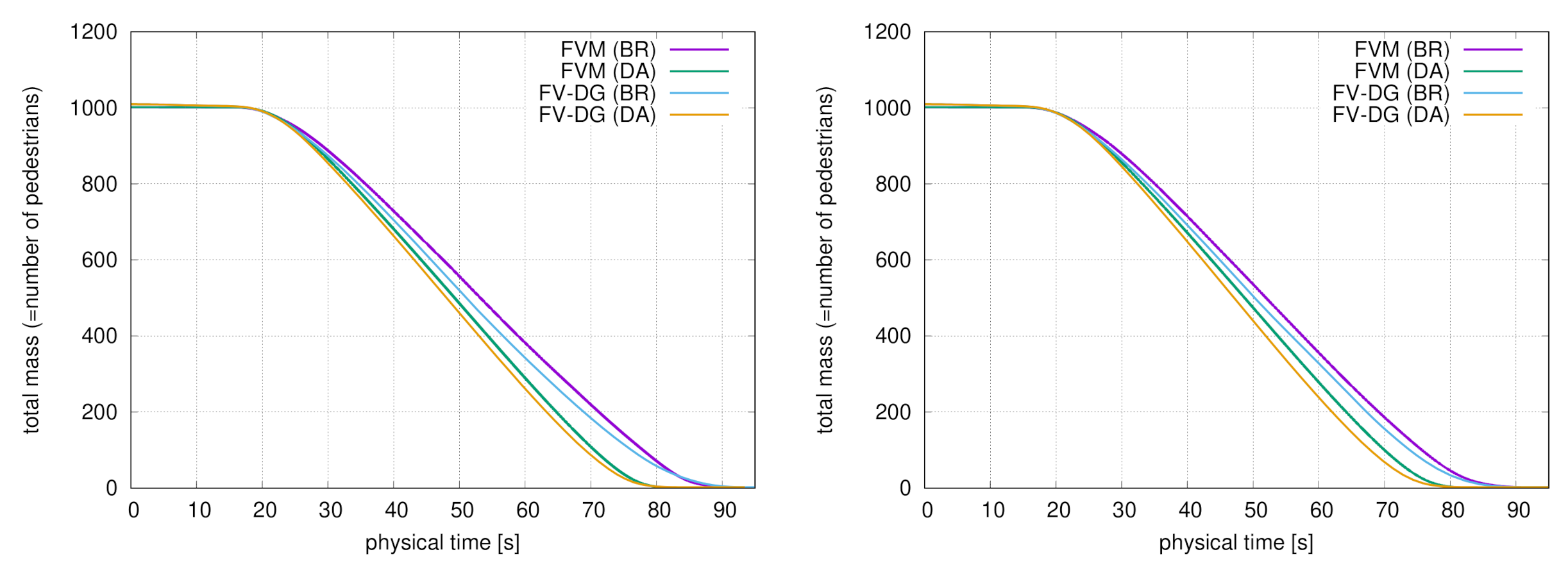
In Figure 7 the density evolution for selected time instants is depicted. Here the local increase of the pedestrian density in the left part of the narrowing and also close to the exit of the domain is noticeable. In Figure 8 the evolution of number of pedestrian in the domain is shown. The main differences are due to the use of the DA or BR algorithms.
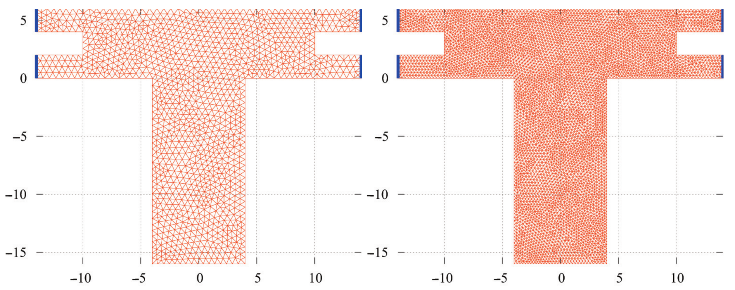
4.4. T-Shape Domain Evacuation
Here we present numerical example for the multiple exits non-convex domain, the so-called T-shape domain, see Figure 9 for details. The -coordinates and the -coordinates of the corners are and , respectively.
The outflow is situated on the vertical right- and left-hand sides of , i.e.,
Moreover, the wall boundary is obviously . The initial condition is set
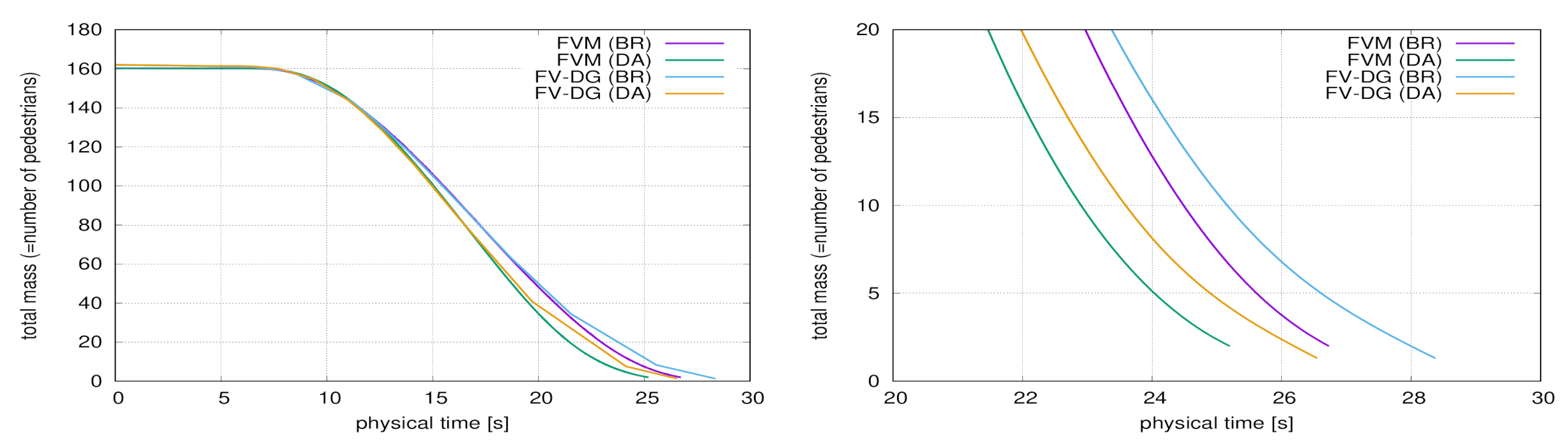
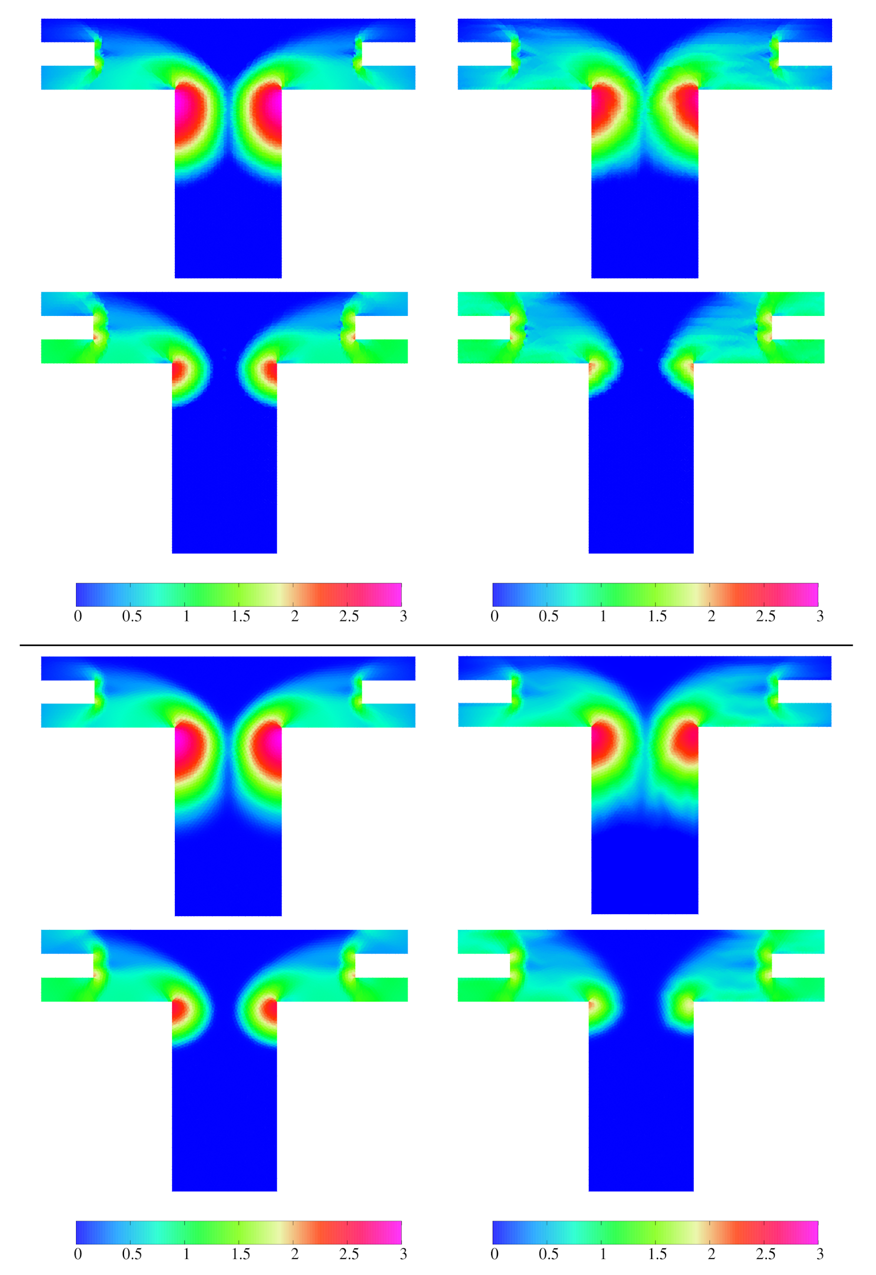
Table 4 shows the computational results for the T-shape domain. There is a small difference in between FV and FV-DG but the results are still in a good agreement from the practical point of view. The evolution of number of pedestrians in T-shape domain is shown in Figure 10. The pedestrian density distribution over the domain for different time instants is depicted in Figure 11.
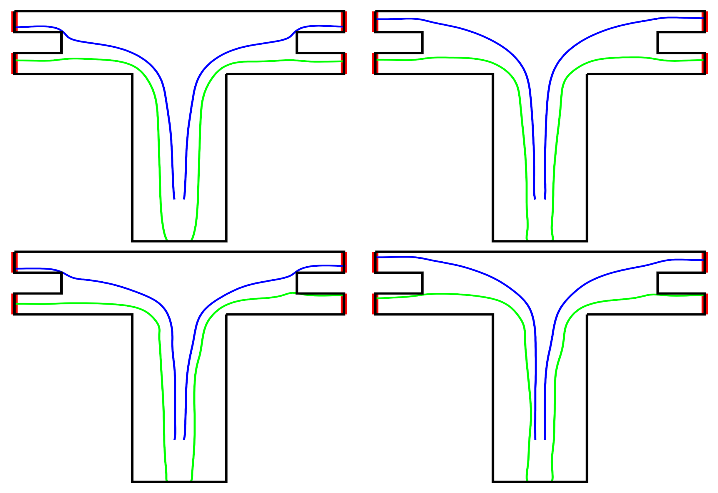
The Figure 12 shows the trajectories of “selected” pedestrians. Trajectories of the pedestrians are given by the solution of the differential equation
with initial condition . The initial condition arranges the pedestrian selection. The Equation (69) is solved by the forward Euler method. Here we use the piecewise constant approximation of obtained from the numerical solution and (see Definitions 1 and 2). The trajectories in Figure 12 show us the influence of the density distribution on the movement of pedestrians and their trajectory, since depends on the density.
Figure 12 (blue trajectories) shows the situation, where more distant outflow is selected, because of the pedestrian density distribution. The initial positions is set . Pedestrians from this position cross the line at time s and reach the more distant exit at time s. The reason is the density in the corners in time s is quite high and pedestrians prefer (dependence of on the density) to get round domains with high density. Whereas pedestrians with initial position cross the line later at time s and reach the nearer exit at time s. The domains with high density at time s are smaller and thus nearer exits are preferred. This corresponds to intuitive imagination of the pedestrian behaviour in real situations.
5. Conclusions
The paper deals with the comparative study of two splitting methods-Splitting Method I and Splitting Method II. They were described and numerically tested for solving several pedestrian flow problems. The FV approach was compared with FV-DG approach. The former use the piece-wise constant approximation together with the explicit time discretization and is advantageous from the implementation point of view. The latter is based on the discontinuous piece-wise polynomial approximation and uses the implicit discretization by space time discontinuous Galerkin method. The FV-DG approach requires the solution of the system of nonlinear algebraic equations, but on the other hand the implicit time discretization together with the high polynomial degree enable us to use the longer time steps. Further the FV-DG approach allow us to use different space grids on different time levels which is useful for adaptive methods.
The alternative method to that proposed by Bornemann and Rasch for the computation of the desired direction of move in (4) based on the Dijkstra’s algorithm was proposed and tested. This method can be considered as a competitive method to the Bornemann–Rasch algorithm for the solution of the Eikonal equation. The key difference is in leaving out the differential formulation given by the Eikonal equation (8) and replacing its iterative solution by the modification of the Dijkstra’s algorithm for the shortest path in a graph. The curvilinear integral in (6) is minimized in the class of piece-wise linear curves given by edges of the triangulation. Compared with the Bornemann–Rasch algorithm (BR) the proposed method has several different properties. Firstly, the method is tolerance free in the distinction from the iterative BR algorithm, where the stopping criterion must be prescribed. Secondly, in the proposed method the computation of the gradient of in vertex P can be avoided by using the direction of the edge which lies on the shortest path from P to the outflow.
The special advantage of presented simulations is that the system of partial differential equations is solved by two different software systems with the results being in the good agreement. This is related to the key word “verification” of the model, i.e., to the question, if the equations are solved “right”. Another step is the question, if we solve the “right” equations, which is related to the notion “validation” of the model. This suppose the comparison with the experimental data. Two ingredients of the proposed methods are original. We use the numerical flux which is the original modification of the Vijayasundaram numerical flux for the Euler equations. Despite the fact that in the distinction from the Euler fluxes the fluxes for the pedestrian flow equations are not homogeneous, we were able to propose the numerical flux of the Vijayasundaram type which is easy to be coded. For details see [8,22]. Further we are able to avoid the numerical solution of the Eikonal equation. This is related to the notion of the fastest path in a graph. The details can be found in [8,27]. We use the triangular finite volumes and the numerical flux mentioned above. In [3] the dual finite volumes are used and the HLL numerical is flux applied. The results can be mutually compared.
Author Contributions
Conceptualization, P.K. and J.F.; Formal analysis, J.F.; Software, P.K.; Visualization, P.K.; Writing—original draft, J.F.; Writing—review and editing, P.K. All authors have read and agreed to the published version of the manuscript.
Funding
This research was funded by IGA UJEP, grant No. UJEP-IGA-TC-2019-53-02-2.
Institutional Review Board Statement
Not applicable.
Informed Consent Statement
Not applicable.
Data Availability Statement
Not applicable.
Acknowledgments
The FV-DG solution of the problem was computed by the software written by Vít Dolejší (see [23]). The authors acknowledge his help in the adaptation of the software for the pedestrian flow problem.
Conflicts of Interest
The authors declare no conflict of interest.
References
- Liu, R.; Fu, Z.; Schadschneider, A.; Wen, Q.; Chen, J.; Liu, S. Modeling the effect of visibility on upstairs crowd evacuation by a stochastic FFCA model with finer discretization. Phys. A Stat. Mech. Appl. 2019, 531, 121723. [Google Scholar] [CrossRef]
- Fu, Z.; Zhan, X.; Luo, L.; Schadschneider, A.; Chen, J. Modeling fatigue of ascending stair evacuation with modified fine discrete floor field cellular automata. Phys. Lett. A 2019, 383, 1897–1906. [Google Scholar] [CrossRef]
- Twarogowska, M.; Goatin, P.; Duvigneau, R. Macroscopic modeling and simulation of room evacuation. Appl. Math. Model. 2014, 38, 5781–5795. [Google Scholar] [CrossRef]
- Buchmueller, S.; Weidmann, U. Parameters of pedestrians, Pedestrian Traffic and Walking Facilities. IVT Schriftenreihe 2007, 132. [Google Scholar] [CrossRef]
- Bellomo, N.; Marasco, A.; Romano, A. From the modelling of driver’s behavior to hydrodynamics models and problems of traffic flow. Nonlinear Anal. RWA 2002, 3, 339–363. [Google Scholar] [CrossRef]
- Venuti, F.; Bruno, L.; Bellomo, N. Crowd dynamics on a moving platform: Mathematical modelling and application to lively footbridges. Math. Comp. Model. 2007, 45, 252–269. [Google Scholar] [CrossRef]
- Bellomo, N.; Dogbé, C. On the modelling crowd dynamics from scaling to hyperbolic macroscopic models. Math. Model. Methods Appl. Sci. 2008, 18, 1317–1345. [Google Scholar] [CrossRef] [Green Version]
- Dolejší, V.; Felcman, J.; Kubera, P. FV–DG Method for the Pedestrian Flow Problem. Comput. Fluids 2019, 183, 1–15. [Google Scholar] [CrossRef]
- Jiang, Y.; Zhang, P.; Wong, S.; Liu, R. A higher-order macroscopic model for pedestrian flows. Phys. A Stat. Mech. Appl. 2010, 389, 4623–4635. [Google Scholar] [CrossRef]
- Payne, H. Models of Freeway Traffic and Control; Simulation Councils, Incorporated: La Jolla, CA, USA, 1971. [Google Scholar]
- Whitham, G. Linear and Nonlinear Waves; Pure and Applied Mathematics; Wiley: Hoboken, NJ, USA, 1974. [Google Scholar]
- Berres, S.; Ruiz-Baier, R.; Schwandt, H.; Tory, E. An adaptive finite-volume method for a model of two-phase pedestrian flow. Netw. Heterog. Media 2011, 6, 401–423. [Google Scholar] [CrossRef]
- Dridi, M.H. Simulation of high density pedestrian flow: Microscopic model. Open J. Model. Simul. 2015, 3, 81–95. [Google Scholar] [CrossRef] [Green Version]
- Marno, P. Crowded-Macroscopic and Microscopic Models for Pedestrian Dynamics. Ph.D. Thesis, University of Reading, Reading, UK, 2002. [Google Scholar]
- Felcman, J.; Kubera, P. A cellular automaton model for a pedestrian flow problem. Math. Model. Nat. Phenom. 2021, 16, 11. [Google Scholar] [CrossRef]
- Dogbe, C. On the modelling of crowd dynamics by generalized kinetic models. J. Math. Anal. Appl. 2012, 387, 512–532. [Google Scholar] [CrossRef] [Green Version]
- Toro, E.F. Riemann Solvers and Numerical Methods for Fluid Dynamics; Springer: Berlin, Germany, 1997. [Google Scholar]
- Dijkstra, E.W. A note on two problems in connexion with graphs. Numer. Math. 1959, 1, 269–271. [Google Scholar] [CrossRef] [Green Version]
- Cormen, T.H.; Leiserson, C.E.; Rivest, R.L.; Stein, C. Introduction to Algorithms, 2nd ed.; The MIT Press: Cambridge, MA, USA, 2001. [Google Scholar]
- Bornemann, F.; Rasch, C. Finite-element Discretization of Static Hamilton-Jacobi Equations based on a Local Variational Principle. Comput. Vis. Sci. 2006, 9, 57–69. [Google Scholar] [CrossRef] [Green Version]
- Felcman, J.; Dolejší, V.; Kubera, P. Discontinuous Galerkin Method for the Pedestrian Flow Problem. In ICNAAM 2017 AIP Conference Proceedings 1978:1; Simos, T.E., Tsitouras, C., Eds.; American Institute of Physics: Melville, NY, USA, 2018; pp. 0300191–0300194. [Google Scholar] [CrossRef]
- Kubera, P.; Felcman, J. On a numerical flux for the pedestrian flow equations. J. Appl. Math. Stat. Inform. 2015, 11, 79–96. [Google Scholar] [CrossRef] [Green Version]
- Dolejší, V.; Feistauer, M. Discontinuous Galerkin Method; Springer: New York, NY, USA, 2015. [Google Scholar]
- Petrášová, T. Application of the Dijkstra’s Algorithm in the Pedestrian Flow Problem. Bachelor’s Thesis, Charles University in Prague, Prague, Czech Republic, 2016. [Google Scholar]
- Deuflhard, P. Newton Methods for Nonlinear Problems; Springer Series in Computational Mathematics; Springer: Berlin/Heidelberg, Germany, 2004; Volume 35. [Google Scholar]
- Dolejší, V.; Roskovec, F.; Vlasák, M. Residual based error estimates for the space-time discontinuous Galerkin method applied to the compressible flows. Comput. Fluids 2015, 117, 304–324. [Google Scholar] [CrossRef]
- Felcman, J.; Kubera, P. On the Eikonal Equation in the Pedestrian Flow Problem. In ICNAAM 2016 AIP Conference Proceedings 1863:1; Simos, T.E., Tsitouras, C., Eds.; American Institute of Physics: Melville, NY, USA, 2017; pp. 5600241–5600244. [Google Scholar]
Figure 1.
Examples of finite volume meshes with one circular obstacle at point with radius m (top) and with three circular obstacles at points , and with radius m (bottom).
Figure 1.
Examples of finite volume meshes with one circular obstacle at point with radius m (top) and with three circular obstacles at points , and with radius m (bottom).

Figure 2.
Domain with one obstacle, FV(BR), FV(DA) (top) and FV-DG(BR), FV-DG(DA) (bottom). Density distribution at time s obtained on the finest meshes.
Figure 2.
Domain with one obstacle, FV(BR), FV(DA) (top) and FV-DG(BR), FV-DG(DA) (bottom). Density distribution at time s obtained on the finest meshes.

Figure 3.
Domain with one circular obstacle, the time evolution of the total number of pedestrians for the finest grid (FVM) and (FV-DG), total view (left) and the detailed view close to the end of the evacuation (right).
Figure 3.
Domain with one circular obstacle, the time evolution of the total number of pedestrians for the finest grid (FVM) and (FV-DG), total view (left) and the detailed view close to the end of the evacuation (right).

Figure 4.
Domain with three obstacles, FV(BR), FV(DA) (top) and FV-DG(BR), FV-DG(DA) (bottom). Density distribution at time s obtained on the finest meshes.
Figure 4.
Domain with three obstacles, FV(BR), FV(DA) (top) and FV-DG(BR), FV-DG(DA) (bottom). Density distribution at time s obtained on the finest meshes.

Figure 5.
Domain with three circular obstacles, the time evolution of the total number of pedestrians for the finest grid = 11,660 (FV) and = 11,636 (FV-DG), total view (left) and the detailed view close to the end of the evacuation (right).
Figure 5.
Domain with three circular obstacles, the time evolution of the total number of pedestrians for the finest grid = 11,660 (FV) and = 11,636 (FV-DG), total view (left) and the detailed view close to the end of the evacuation (right).

Figure 6.
H-shape domain, examples of the computational grids (FV-DG) with (left) and = 12,742 (right) elements, the exits at the right-hand side bottom corner are marked by the blue color.
Figure 6.
H-shape domain, examples of the computational grids (FV-DG) with (left) and = 12,742 (right) elements, the exits at the right-hand side bottom corner are marked by the blue color.

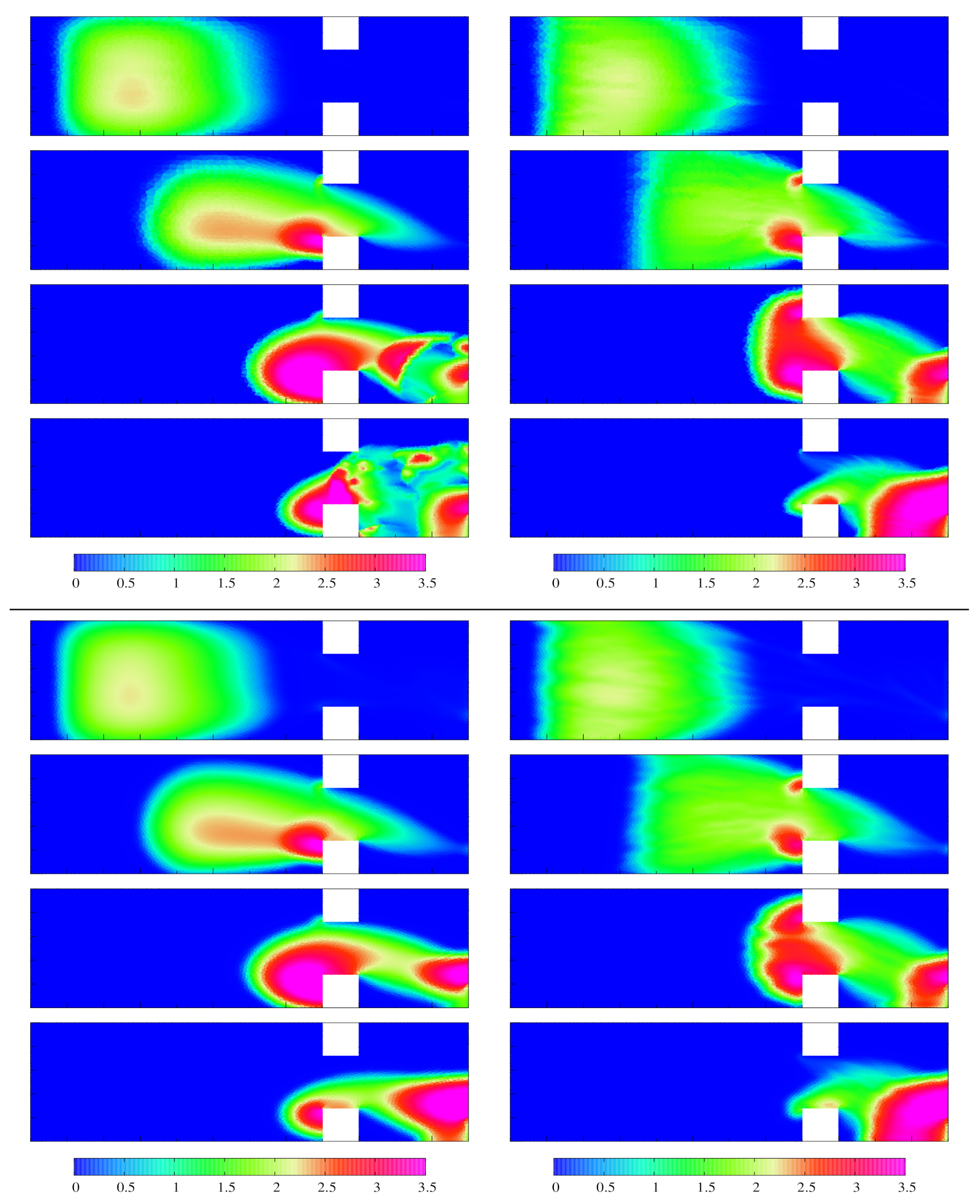
Figure 7.
H-shape domain, FV(BR), FV(DA) (top) and FV-DG(BR), FV-DG(DA) (bottom). Density distribution obtained on the finest meshes at time s.
Figure 7.
H-shape domain, FV(BR), FV(DA) (top) and FV-DG(BR), FV-DG(DA) (bottom). Density distribution obtained on the finest meshes at time s.

Figure 8.
H-shape domain, the time evolution of the total number of pedestrians for the finest grid (left) and for the coarsened grid (right).
Figure 8.
H-shape domain, the time evolution of the total number of pedestrians for the finest grid (left) and for the coarsened grid (right).

Figure 9.
T-shape domain, computational grids (FV-DG) with (left) and = 10,848 (right) elements, the exits are marked by the blue color.
Figure 9.
T-shape domain, computational grids (FV-DG) with (left) and = 10,848 (right) elements, the exits are marked by the blue color.

Figure 10.
T-shape domain, the time evolution of the total number of pedestrians for the finest grid = 10,310 (FVM) and = 10,848 (FV-DG), total view (left) and the detailed view close to the end of the evacuation (right).
Figure 10.
T-shape domain, the time evolution of the total number of pedestrians for the finest grid = 10,310 (FVM) and = 10,848 (FV-DG), total view (left) and the detailed view close to the end of the evacuation (right).

Figure 11.
T-shape domain, FV(BR), FV(DA) (top) and FV-DG(BR), FV-DG(DA) (bottom). Density distribution obtained on the finest meshes at time s.
Figure 11.
T-shape domain, FV(BR), FV(DA) (top) and FV-DG(BR), FV-DG(DA) (bottom). Density distribution obtained on the finest meshes at time s.

Figure 12.
T-shape domain pedestrian trajectories. First row FV in order Bornemann-Rasch algorithm and Dijkstra’s algorithm, second row FV-DG method in the same order. Pedestrian trajectories for starting position (blue color) and , respectively (green color). The pedestrians starting at cross the line at time s and reach the more distant exit at time s. The pedestrians starting at cross the line at time s and reach the nearer exit at time s.


Table 1.
Domain with one obstacle, FV (Splitting Scheme I-left) and FV-DG (Splitting Scheme II-right)-Comparison of computations on series of meshes, , evacuation time with Bornemann-Rasch algorithm for the determination of in (8), evacuation time with Dijkstra’s algorithm for the determination of in (6).
| [s] | [s] | [s] | [s] | ||
|---|---|---|---|---|---|
| 1114 | 35.0 | 35.1 | 1126 | 35.2 | 36.2 |
| 2148 | 34.7 | 34.7 | 2132 | 35.2 | 36.1 |
| 4610 | 34.9 | 34.7 | 4627 | 35.0 | 35.5 |
| 9056 | 34.8 | 34.7 | 9082 | 34.8 | 35.4 |
Table 2.
Domain with three obstacles, FV (left) and FV-DG (right)-Comparison of computations on the series of meshes, , evacuation time with Bornemann-Rasch algorithm, evacuation time with Dijkstra’s algorithm.
Table 2.
Domain with three obstacles, FV (left) and FV-DG (right)-Comparison of computations on the series of meshes, , evacuation time with Bornemann-Rasch algorithm, evacuation time with Dijkstra’s algorithm.
| [s] | [s] | [s] | [s] | ||
|---|---|---|---|---|---|
| 1622 | 34.5 | 34.9 | 1653 | 35.0 | 35.6 |
| 2653 | 34.6 | 34.5 | 2616 | 34.9 | 35.5 |
| 7115 | 34.7 | 34.5 | 7084 | 34.9 | 35.1 |
| 11,660 | 35.0 | 34.6 | 11,636 | 34.7 | 35.0 |
Table 3.
H-shape domain, FV (left) and FV-DG (right), , evacuation time with Bornemann-Rasch algorithm, evacuation time with Dijkstra’s algorithm.
Table 3.
H-shape domain, FV (left) and FV-DG (right), , evacuation time with Bornemann-Rasch algorithm, evacuation time with Dijkstra’s algorithm.
| [s] | [s] | [s] | [s] | ||
|---|---|---|---|---|---|
| 2994 | 90.8 | 81.0 | 2941 | 87.5 | 79.1 |
| 12,835 | 90.5 | 81.0 | 12,742 | 90.5 | 80.0 |
Table 4.
T-shape domain, FV (left) and FV-DG (right), , evacuation time with Bornemann-Rasch algorithm, evacuation time with Dijkstra’s algorithm.
Table 4.
T-shape domain, FV (left) and FV-DG (right), , evacuation time with Bornemann-Rasch algorithm, evacuation time with Dijkstra’s algorithm.
| [s] | [s] | [s] | [s] | ||
|---|---|---|---|---|---|
| 2678 | 26.7 | 25.4 | 2578 | 28.1 | 27.9 |
| 10,310 | 26.7 | 25.2 | 10,848 | 28.4 | 26.6 |
Publisher’s Note: MDPI stays neutral with regard to jurisdictional claims in published maps and institutional affiliations. |
© 2021 by the authors. Licensee MDPI, Basel, Switzerland. This article is an open access article distributed under the terms and conditions of the Creative Commons Attribution (CC BY) license (https://creativecommons.org/licenses/by/4.0/).
Share and Cite
MDPI and ACS Style
Kubera, P.; Felcman, J. On the Verification of the Pedestrian Evacuation Model. Mathematics 2021, 9, 1525. https://doi.org/10.3390/math9131525
AMA Style
Kubera P, Felcman J. On the Verification of the Pedestrian Evacuation Model. Mathematics. 2021; 9(13):1525. https://doi.org/10.3390/math9131525
Chicago/Turabian StyleKubera, Petr, and Jiří Felcman. 2021. "On the Verification of the Pedestrian Evacuation Model" Mathematics 9, no. 13: 1525. https://doi.org/10.3390/math9131525
Note that from the first issue of 2016, this journal uses article numbers instead of page numbers. See further details here.