Article

Generating Up-to-Date Crop Maps Optimized for Sentinel-2 Imagery in Israel

1
Agricultural Research Organization, Volcani Institute, Institute of Soil, Water and Environmental Sciences, HaMaccabim Road 68, P.O. Box 15159, Rishon LeZion 7528809, Israel
2
The Robert H. Smith Institute for Plant Sciences and Genetics in Agriculture, The Hebrew University of Jerusalem, P.O. Box 12, Rehovot 7610001, Israel
*
Author to whom correspondence should be addressed.
Remote Sens. 2021, 13(17), 3488; https://doi.org/10.3390/rs13173488
Submission received: 26 June 2021 / Revised: 28 August 2021 / Accepted: 30 August 2021 / Published: 2 September 2021
(This article belongs to the Special Issue Theory and Application of Machine Learning in Remote Sensing)

Abstract

:
The overarching aim of this research was to develop a method for deriving crop maps from a time series of Sentinel-2 images between 2017 and 2018 to address global challenges in agriculture and food security. This study is the first step towards improving crop mapping based on phenological features retrieved from an object-based time series on a national scale. Five main crops in Israel were classified: wheat, barley, cotton, carrot, and chickpea. To optimize the object-based classification process, different characteristics and inputs of the mean shift segmentation algorithm were tested, including vegetation indices, three-band combinations, and high/low emphasis on the spatial and spectral characteristics. Four known vegetation indices (VIs)-based time series were tested. Additionally, we compared two widely used machine learning methods for crop classification, support vector machine (SVM) and random forest (RF), in addition to a newer classifier, extreme gradient boosting (XGBoost). Lastly, we examined two accuracy measures—overall accuracy (OA) and area under the curve (AUC)—in order to optimally estimate the accuracy in the case of imbalanced class representation. Mean shift best performed when emphasizing both the spectral and spatial characteristics while using the green, red, and near-infrared (NIR) bands as input. Both accuracy measures showed that RF and XGBoost classified different types of crops with significantly greater success than achieved by SVM. Nevertheless, AUC was better able to represent the significant differences between the classification algorithms than OA was. None of the VIs showed a significantly higher contribution to the classification. However, normalized difference infrared index (NDII) with XGBoost classifier showed the highest AUC results (88%). This study demonstrates that the short-wave infrared (SWIR) band with XGBoost improves crop type classification results. Furthermore, the study emphasizes the importance of addressing imbalanced classification datasets by using a proper accuracy measure. Since object-based classification and phenological features derived from a VI-based time series are widely used to produce crop maps, the current study is also relevant for operational agricultural management and informatics at large scales.

Graphical Abstract

1. Introduction

Agriculture plays a crucial role in both water management and food security. Irrigated agriculture is one of the most significant water consumers [1], and agricultural production is key to food supply. Due to the impact of agriculture on the world’s resources, it must be optimally managed to secure our future. Identifying which crop is grown where and when is essential for better decision-making regarding water and fertilization. For example, crop maps can facilitate crop-specific water consumption estimates [2,3] and provide a basis for regional yield forecasting [4]. Therefore, decision-makers may rely on crop maps as a reliable tool to facilitate better agricultural management.
In recent decades, studies have shown that spaceborne remote sensing can be used for accurate crop mapping. Among the satellites used for crop mapping are Landsat, SPOT, and MODIS. Imagery from these satellites is offered to the public at no cost, yet they provide either high spatial or high temporal resolutions, but not both [5]. In 2015 and 2017, the earth observation satellites Sentinel-2A and Sentinel-2B, respectively, were launched as part of the European Copernicus program. These satellites provide public-domain imagery at a combined temporal resolution of five days, a spatial resolution of 10–20 m in visible, near-infrared (NIR), red edge, and short-wave infrared (SWIR), positioning them as potentially suitable for monitoring land use in agriculture.
Satellite images of fields with large spectral in-field variability can lead to crop misclassification; more than one crop type is tagged inside one field. One way to overcome this problem is by using object-based classification. This approach to crop classification generates objects representing the boundaries of the agricultural fields through a process termed segmentation. Segmentation techniques use the spectral and spatial characteristics of the image to differentiate between objects [6,7,8]. Large spectral variability might limit the ability to identify crops when using only spectral information [9]. Therefore, using the unique crop phenological features can overcome this limitation because crops often have different seasonal variations [10,11]. The phenology features can be automatically extracted using feature extraction methods from vegetation indices (VIs) time series [12]. A widely used VI is the normalized difference vegetation index (NDVI) [13]. This index uses the red and NIR bands to assess green vegetation and indicate vegetation productivity as well as phenological changes. However, NDVI is sensitive to soil and atmospheric influences, such as soil color and brightness, as well as clouds and shadow [14]. Additionally, from a certain phenology stage, NDVI is less sensitive to the green leaf area of the crop and, therefore, will peak sooner than the crop leaf area will [15]. NDVI time series from satellite data was used for crop classification [16,17,18] and specifically, with Sentinel-2 imagery [6,19]. An additional VI is the optimized soil-adjusted vegetation index (OSAVI) [20]. OSAVI is a simplified version of the SAVI, and is based on the red and NIR bands, with a reduced soil background effect. Even though SAVI has been used for land cover classification [21] as well as crop classification [22,23], OSAVI is not generally used for crop classification, and its previous applications include, for example, detection of chlorophyll content and above-ground biomass [14,24]. The VI normalized difference red edge index (NDRE) [25] uses the NIR band and the red edge band, which is less translucent to leaves. Eitel et al. [26] compared NDRE with other VIs, such as NDVI, and showed that NDRE improves forest stress monitoring from RapidEye imagery. In the context of crop classification, Ustuner et al. [27] demonstrated that NDRE had a greater contribution compared with other indices such as NDVI to crop classification from RapidEye imagery. Another VI is normalized difference infrared index (NDII) [28]. NDII uses the NIR and SWIR bands and is mainly correlated with water content in vegetation. NDII was used successfully to extract rice from remote sensing images [29,30] and showed a higher ability than demonstrated by NDVI to do so [29]. In addition, NDII was used, among other bands, for crop classification based on Sentinel-2 imagery [23]. SWIR bands have a high contribution to crop classification performance [10,31], and VIs that are based on SWIR bands are helpful for crop identification [8].
Subsequently, the segmentation of plot boundaries, together with the extraction of crop phenological characteristics, can facilitate accurate crop classification. Categorizing segments into crop types in the classification process can be achieved using many classification methods. Nonlinear multiclass classification methods can detect the nonlinear relations between crop type and cropping patterns. Therefore, to distinguish between crops with common development patterns and similar spectral responses, machine learning algorithms are growing in popularity [32,33,34,35,36,37,38].
The overarching aim of this study was to develop a process to automatically generate crop maps for Israel from a time series of Sentinel-2 imagery. This process included several steps: segmentation, VI time series calculation, phenology features extraction, classification, and evaluation. Each one of those steps was performed in several ways. Here, we compare the performance of different combinations of parameters (i.e., high/low spectral or spatial) and inputs (i.e., three optical bands or NDVI greyscale band) to the Mean Shift segmentation technique. In addition, to determine the best input for classification, we compare time series of different VIs, such as NDVI, OSAVI, NDRE, and NDII, in addition to different phenology features. Moreover, we compare three machine learning methods—random forest (RF), support vector machine (SVM), and extreme gradient boosting (XGBoost)—for crop classification. Lastly, we test and discuss two accuracy measures, AUC and OA, to evaluate imbalanced classification.

2. Materials and Methods

2.1. Sentinel-2 Data Acquisition, Preprocessing, and VIs Calculation

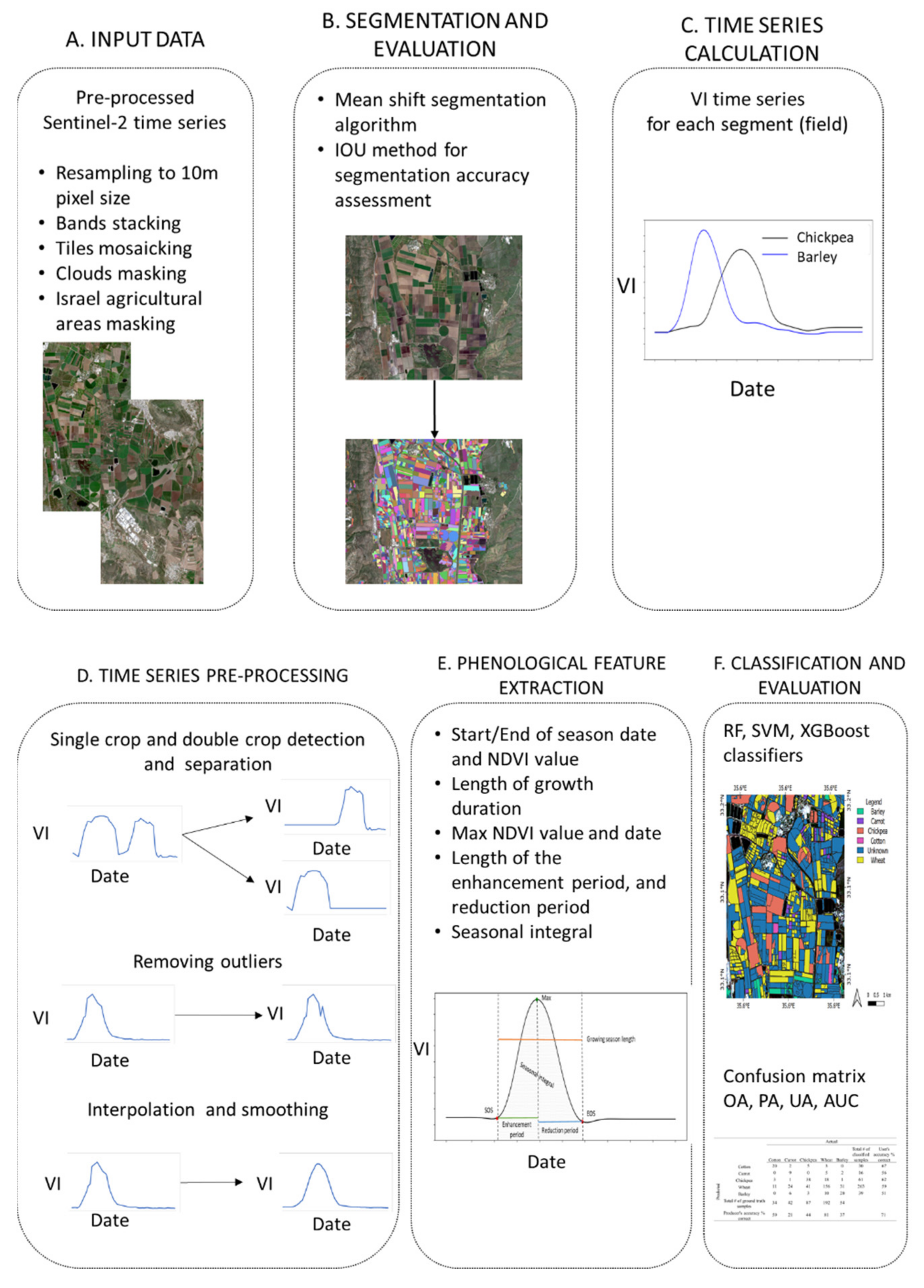
A time series of Sentinel-2 images from 119 dates between October 2017 and September 2019 was acquired from the Copernicus Open Access Hub (https://scihub.copernicus.eu/ accessed on 1 September 2021). The data were obtained for seven Sentinel-2 L2A tiles (36SXB, 36SYB, 36SXA, 36SYA, 36RXV, 36RXU, 36RXT) in order to achieve nationwide coverage of Israel (Figure 1). The tiles were preprocessed using ERDAS Imagine 2018 (Hexagon Geospatial, Peachtree Corners Circle Norcross). The resolution of 20 m bands was resampled into 10 m using the nearest neighbor algorithm. All bands from the same tile were stacked into one tile to create a 12-band tile, and all tiles from the same date were mosaicked to create an image of the total area of Israel. Finally, clouds were masked to create a cloudless mosaic using the Sentinel-2 level 2A product that includes a cloud detection flag. The images were also masked by the borders of Israel's agricultural area [39]. This way, we created 10 m cloud-free mosaics for a period of two years (Figure 2A). Then, four VIs: NDVI, OSAVI, NDRE, and NDII (Appendix A) were calculated for each one of the 119 mosaics (Figure 2B).

2.2. Segmentation

Object-based classification begins with the creation of objects in a process named segmentation. The segmentation process groups similar adjacent pixels into an object for a joint classification. In crop classification, ideally, each object represents the boundaries of a different agricultural field.
Mean shift segmentation [40] is a nonparametric iterative technique that uses kernel density estimation (KDE). This algorithm has two bandwidth parameters—spectral and spatial. Satellite images are represented as a three-dimensional matrix, employing length, height/width, and spectral bands. The space of the matrix is known as the spatial domain, and the spectral information is known as the range domain. The values of the spectral and spatial parameters determine the spectral and spatial distance between pixels in the range and spatial domains.
Mean shift segmentation was performed using ArcGIS Pro (ESRI, West Redlands, CA, USA) (Figure 2C). In this platform, the spectral and spatial parameters are represented according to the level of importance (in the range of 1–20) given to the spectral differences and the importance given to the proximity, respectively. In this study, these parameters are referred to as spectral and spatial characteristics of pixels within an object. When the parameter value is closer to 20, the emphasis of the parameter is greater, and the importance given to the spectral or spatial characteristics is greater. Therefore, high importance will result in greater similarity of pixels within an object compared with a parameter value closer to 1. Six different combinations of characteristics importance and inputs (Table 1) were assessed for the mean shift algorithm. These inputs were chosen due to the relatively high spatial resolution of the bands used to calculate them (10 m), and the emphasis on the characteristics was selected since this ratio performed well for Sentinel-2 image segmentation [31]. As reference data, polygons of field boundaries were digitized. To generate these polygons, we used six Sentinel-2 images and created 350 polygons for each one of them. To evaluate the segmentation accuracy, segmentation outputs were compared to the compatible reference polygons using the intersection over union (IoU) method [41]. IoU measures the similarity between two segments by dividing the area of overlap by the area of the union of the two segments. This process was repeated six times for the following dates: 31 January 2018, 16 April 2018, 9 August 2018, 31 January 2019, 11 April 2019, and 9 August 2019. To test if there is a significant difference between at least two of the combinations, analysis of variance (ANOVA) was performed, and to test whether there is one combination that is significantly different than the others, a Tukey's post hoc analysis [42,43] was performed. The statistical tests were performed using the Python StatsModels statistics package [44]. Finally, 24 images, one per month with minimal cloud coverage, were segmented into objects using input Combination 1.

2.3. Time Series Analysis

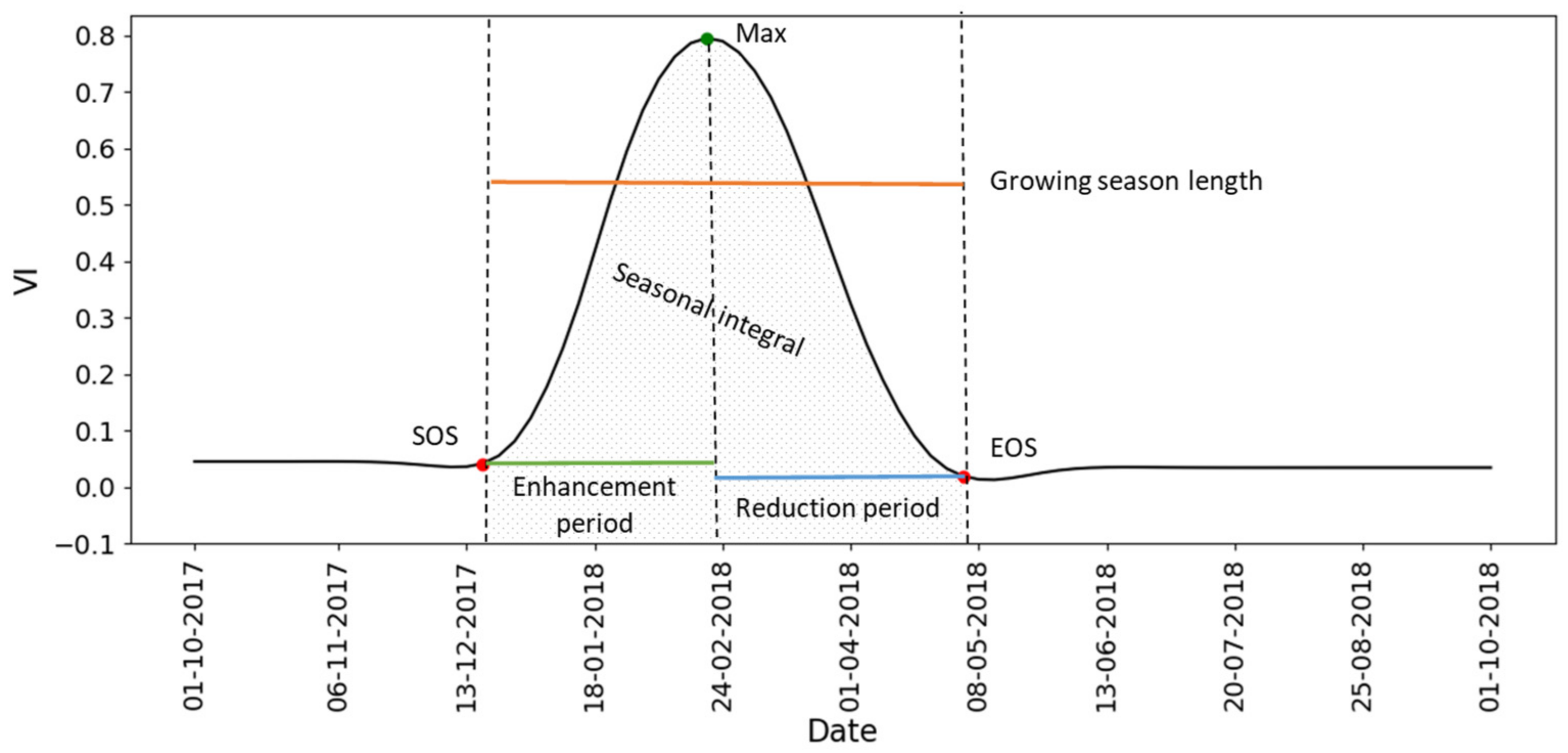
For each one of the 119 images and each one of the VIs, the average pixel value inside the area of each segment was calculated to create a VI time series for each field. The results were four time series for every field—one for each VI. Noise was removed from the VI time series (Figure 2D) using the Python Pandas package [45]. First, it was determined whether one crop was grown during the growing season or two crops were grown one after the other during the growing season in each of the fields. A field-specific sample was considered as a single crop sample if the VI time series contained a single maximum point, and a double-crop sample if it contained two maximum points that were at least 75 days apart and had a local minimum point between them. In the case of the latter, the VI time series of the sample was split into two; one for each crop cycle. Then, all outliers (VI values that were out of trend) were removed. Finally, a Whittaker interpolation was performed for gap filling, followed by Whittaker smoothing to smooth the data [46], using RStudio version 1.2.5033 [47]. The VIs time series were used as the input for the feature extraction process (Figure 2E). Eleven phenological features that represent the unique crops pattern were extracted: the crop start of season (SOS) and end of season (EOS) dates and VI values, the growing season length, the maximum VI date and value, the crop enhancement and reduction periods, the seasonal integral, and the geographic location of the plot. The essential features that served as the basis for most of the other features are the crop start of season (SOS) and end of season (EOS) dates and VI values. To detect those features automatically, we used a modified approach based on a moving average developed by Reed et al. [48]. This method uses a five-point moving average such that the first point is the average of the first five points from the VI time series; the next point is the average of five points following a shift by one point forward, and so on. In this method, the SOS and EOS are the points where the VI time series crosses the moving-average curve or the reverse moving-average curve, respectively.
Once the SOS and EOS dates and the corresponding VI values were extracted, we extracted the remaining features: the growing season length, which is the distance between the SOS and EOS dates; the maximum VI value of the growing season, as well as the date when the growing season reaches its maximum; the crop enhancement and reduction periods, which are the distances from the SOS and EOS dates to the maximum VI date, respectively; the seasonal integral, which is the area below the VI curve between the SOS and EOS (Figure 3), and lastly, the geographic location of the plot (Figure 4). We hypothesized that some crops would be more abundant in specific regions and used the K-means [49] clustering technique to assign every sample to a cluster based on the sample's coordinates. At the end of the process, four datasets, one for each VI, were created. Each one of the datasets contained the phenological features of all the fields.
The phenological signature of each crop was calculated to compare how different features were pronounced in every crop. Therefore, we computed the mean standard score (the distance of the result from the mean in standard deviation units) of each crop by each feature using the Python Scikit-learn package. Since the standard score has slightly different interpretations depending on whether the feature's distribution is normal or not, the Kolmogorov–Smirnov test was performed using the Python Scipy package to determine the normality of the distribution.

2.4. Classification and Accuracy Assessment

Using the Python Scikit-learn package, three classification algorithms (i.e., RF, SVM, XG Boosting) were tested to determine the best VI dataset and classification algorithm for crop classification (Figure 2F): 1361 fields of five crops in Israel were selected to train and test the model. We used crop type polygons from the Ministry of Agriculture [39] that demark the boundaries of each field and the crop type that is grown in that field to assign the type of crop to each segment, using the k-dimensional tree (k-d tree) algorithm [50]. These polygons were created manually from an annual survey carried out by the Ministry of Agriculture [39]. Comparing these polygons to information collected directly from farmers shows that the polygons are reliable but do not cover all of the agricultural areas of Israel.
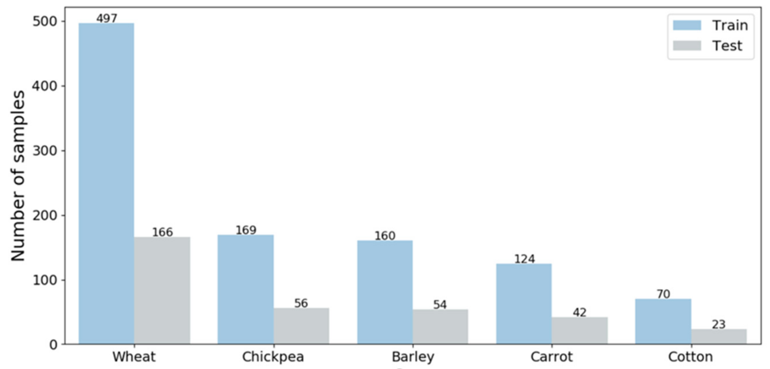
The four VI datasets were split into 75% train dataset and 25% test dataset (Figure 4).
The effect of each phenology feature on the RF and XGBoost classifiers was assessed using the Python Scikit-learn package. The importance was determined by checking how randomizing each feature (and therefore excluding its impact on the classification) affected the accuracy and then standardizing the result to a scale of 0–1. The present Python libraries cannot find the feature importance for nonlinear SVM because the importance of the features is not directly related to the input features.
Evaluation of the accuracy of each crop classification method is often performed using the overall accuracy (OA) statistic. One of the challenges with assessing the accuracy of the classification is the imbalanced classification. This issue occurs when there is a different number of samples from each class. This uneven distribution causes the classification to be biased or skewed. Since the OA can change according to the data distribution in different columns in the confusion matrix, even when the classification performance does not change [51], it is necessary to use an estimation technique that is insensitive to the imbalance in the dataset. One such method is derived from the receiver operating characteristics (ROCs) by relating to the area under the ROC curve. ROC is a graphic method for presenting different classification results. The y-axis of the ROC graph shows the true positive rate, and the x-axis shows the false positive rate. Points generate the curve; each one of them represents the classification results using a different threshold. The AUC accuracy measure is the calculation of the area under the ROC curve. The traditional use of the ROC curve and the AUC measure is for binary classification, as described above. In order to modify this method to imbalanced multiclass classification problems, a ROC curve is produced for each pair of classes. The AUC in such a case would be the mean AUC from all the pairs [51,52,53,54,55]. Therefore in order to evaluate the classification results, we used both the OA and AUC measures. These measures were used for train, validation, and cross-validation evaluation.
The user's accuracy (UA) and producer's accuracy (PA) measurements were computed for each class, for each VI, and for each classification method. Additionally, OA and AUC measurements were calculated for each VI and classification method with train, test, and 10-fold cross-validation estimations. ANOVA and post hoc Tukey statistical tests at α < 0.05 level were computed to determine whether there was a significant difference between the accuracy results of the VIs input and the classifiers (Figure 2F).

3. Results

3.1. Segmentation

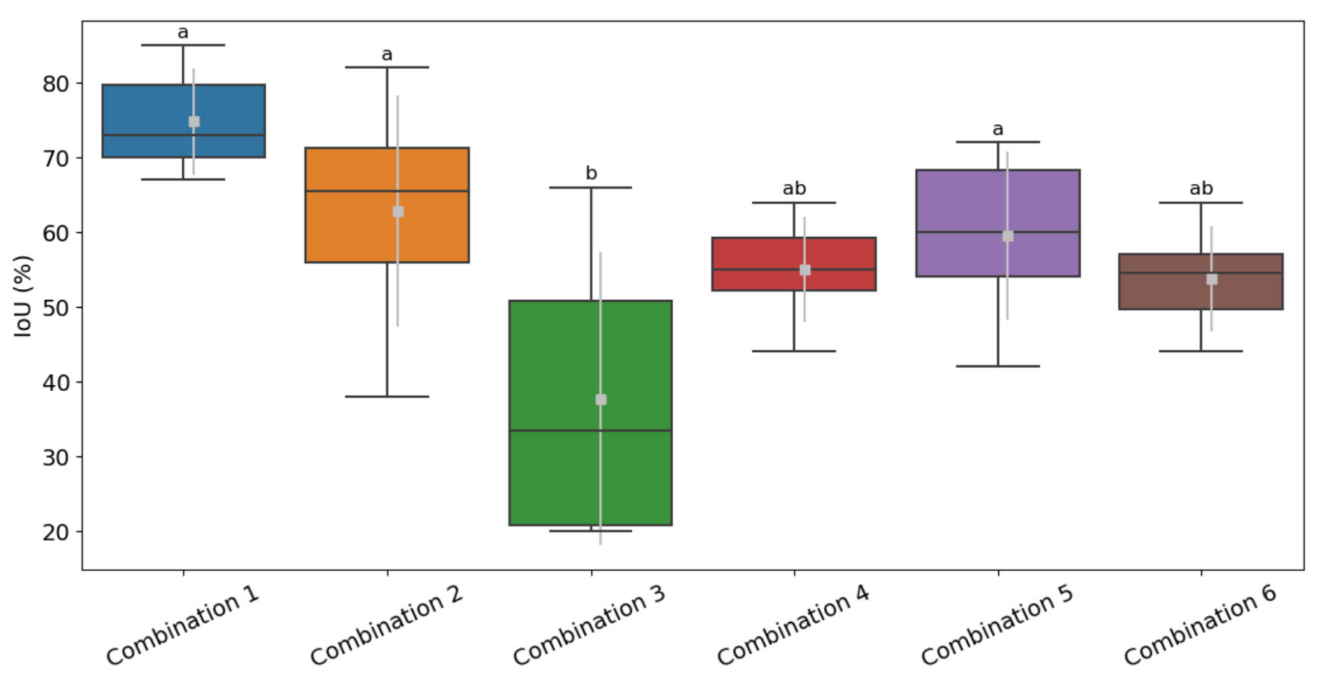
Six combinations of two spectral and spatial characteristics and two types of inputs (Table 1) were compared on six different dates in order to determine the optimal way to use the mean shift segmentation algorithm to segment agricultural plots in Sentinel-2 imagery. We found a statistically significant difference as yielded by one-way ANOVA for the six combinations (F (5,30) = 6, MSE = 150, p = 0.0006). Subsequently, Combination 1 was chosen as the best combination according to its high IoU result and low standard deviation (Figure 5 and Figure 6). This result demonstrates that both the spectral and spatial characteristics of the blue, red, and NIR bands are important for mean shift object segmentation.
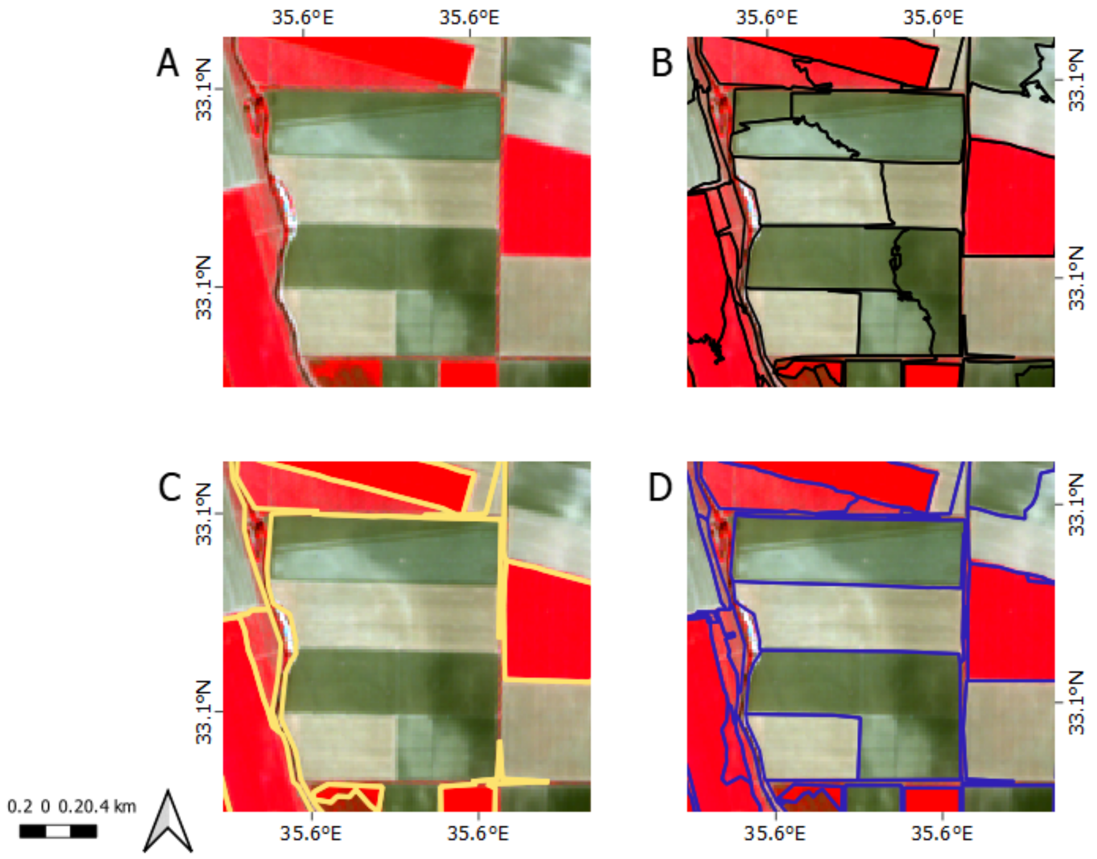
For both NDVI and three-band combination, when the emphasis on both the spectral and spatial characteristics was high (combinations 1 and 4), the number of output segments was similar to that obtained when the emphasis on the spectral characteristic was high and the emphasis on the spatial characteristic was low (combinations 2 and 5). However, when the emphasis on the spatial characteristic was high and the emphasis on the spectral characteristic was low (combinations 3 and 6), the number of segments decreased by more than a half (Figure 7). This trend is presented in Figure 8.

3.2. Phenology Features

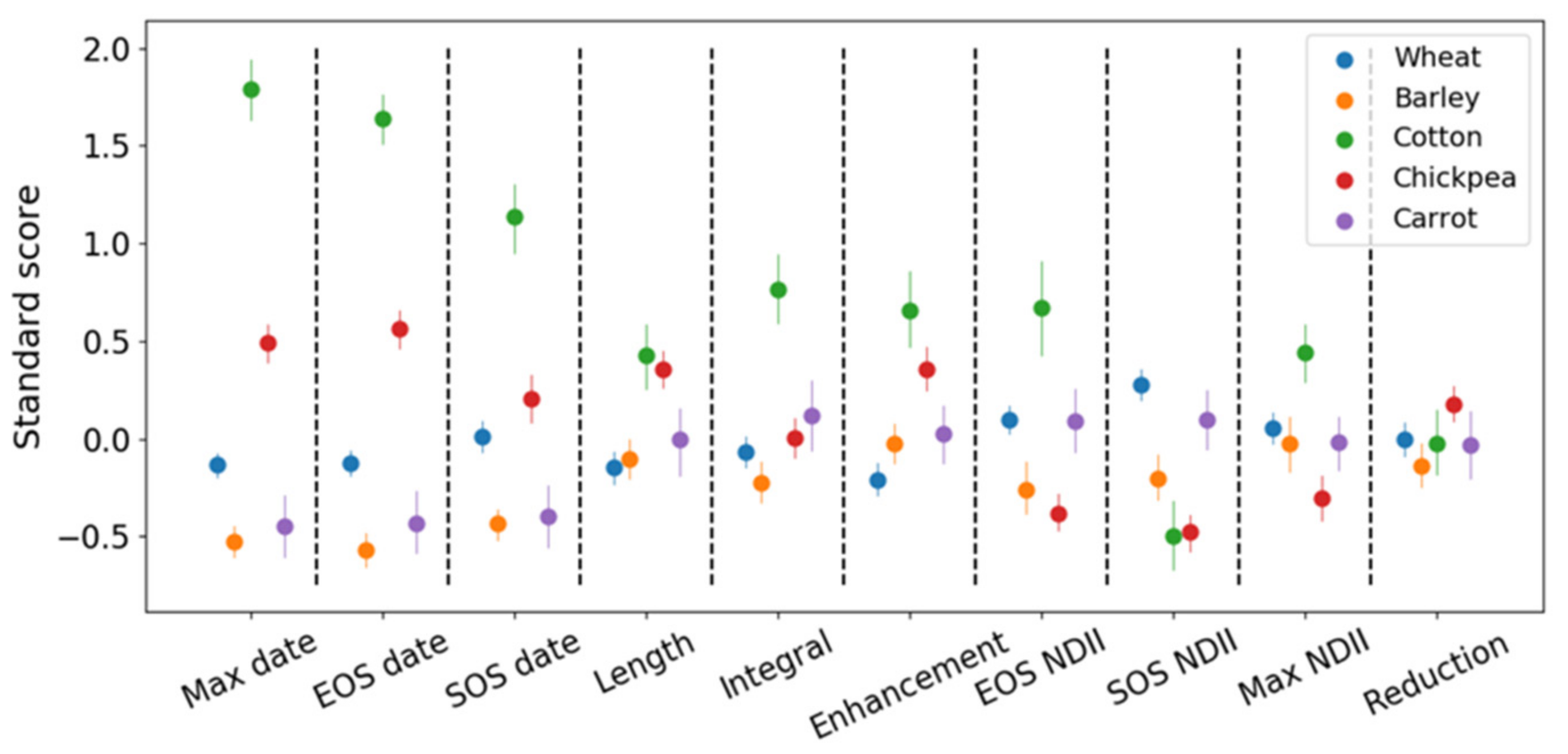
All the date-based features (max date, SOS date, and EOS date) showed a similar trend of crop mean standard score; cotton had a distinctly higher mean standard score compared with the other crops, chickpea and wheat had a rather discrete mean standard scores as well, but barley and carrot had similar mean standard scores. Cotton also showed a particularly high mean standard score of the seasonal integral, the enhancement period, the EOS NDII value, and the max NDII value (Figure 9).
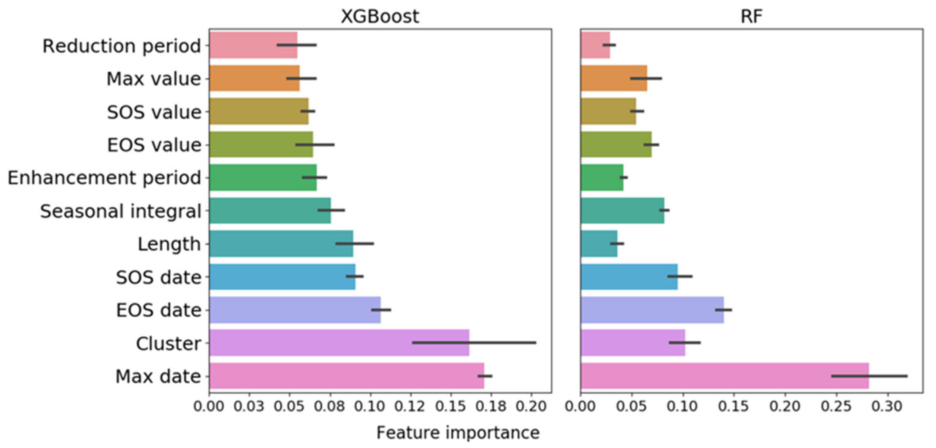
The importance of the phenology features in the RF and XGBoost classifiers is shown in Figure 10. The most important feature of both classification methods was the max date. Additionally, in both methods, the EOS and SOS dates were very important as well. The least important feature of both classifiers was the reduction periods. The rank of the rest of the features was not consistent. For example, growing season length and the geographic location of the field were important in XGBoost but not in RF.

3.3. Classification Results

NDVI, OSAVI, NDRE, and NDII time-series-based phenology features were used as input for the RF, SVM, and XGBoost classifiers. The AUC results were generally higher than the OA results for all the algorithms and VIs (Table 2). One-way ANOVA showed that there was no significant difference between different VIs both for AUC results (F (3, 8) = 0.41, MSE = 12, p = 0.74) and OA results (F (3, 8) = 1.34, MSE = 10, p = 0.33). However, there was a significant difference between the classifiers as shown by one-way ANOVA for AUC results (F (2, 8) = 20.6, MSE = 2.3, p = 0.0004) and OA results (F (2, 8) = 5, MSE = 10.5, p = 0.01). Tukey's post hoc test for both measures determined that the SVM classifier was significantly different from the two other classifiers. Still, there was no significant difference between RF and XGBoost classifiers.
The most accurately classified crop, according to the trends of the UA and PA, was wheat, followed by cotton and chickpea. Barley and carrot were the least accurately classified crops (Table 3). The confusion matrix of NDII time series with XGBoost classifier (Table 4) demonstrates that the majority of confusion was caused when barley, carrot, and chickpea were misclassified as wheat.
Figure 11 shows the final NDII time series with XGBoost classification results. A segment was classified as a certain crop if the classification probability was over 50%, otherwise it was classified as unknown. In some cases, the results were satisfying, but in other cases, one field contained a few segments that were classified as different crops. Moreover, additional crops that were grown in this area were not classified.

4. Discussion

4.1. Segmentation

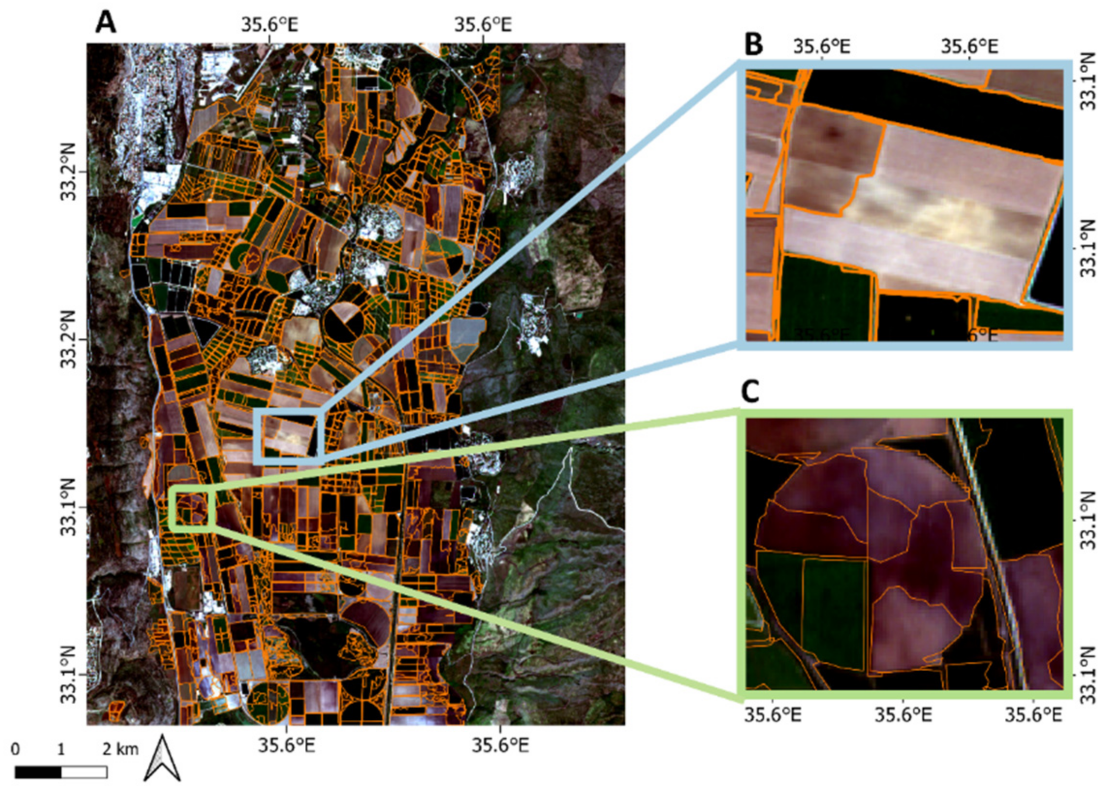
The segments in this study were created using the mean shift algorithm with different inputs and several combinations of emphasis on the spectral and spatial characteristics. A high emphasis on the spectral or spatial characteristics should lead to the creation of more segments. Likewise, a low emphasis on the spectral or spatial characteristics will create a smoother output with fewer segments [56]. Therefore, it was expected that segmentation with a high emphasis on the spectral and spatial characteristics output would have more segments than that obtained when the emphasis on one of the characteristics was low. Additionally, we expected the segmentation output obtained when the emphasis on one of the characteristics was low to have a similar number of segments. The results showed that for both inputs, the number of segments resulting from a high emphasis on the spectral and spatial characteristics was similar to the number of segments obtained when using a high emphasis on the spectral characteristic and low emphasis spatial characteristic. In contrast, the number of segments obtained when using a low emphasis on the spectral characteristic and a high emphasis on spatial characteristic was much lower. This result indicates that the spectral characteristic has more influence on the mean shift segmentation algorithm than has the spatial characteristic. The main segmentation challenges occur in cases of under segmentation where the fields are very similar to one another (such as plowed fields; Figure 6B) or in cases of over segmentation where there is large variability within one field (patches of soil and vegetation or vegetation in different growth stages in one field; Figure 6C). As shown in Figure 8 and from the IoU results, the best and relatively balanced result between over and under segmentation was obtained using a high emphasis on the spectral and spatial characteristics. Therefore, even though the spectral characteristic is more influential, both the spectral and spatial characteristics are important for achieving optimal segmentation results.
Even though segmentation is very common in crop classification, there is little information regarding the segmentation accuracy. Immitzer et al. [31] used a modification of the mean shift segmentation algorithm to determine the boundaries of agriculture fields. By visually evaluating the segmentation results by a trial-and-error approach, they concluded that the pixels in each segment should be less spectrally similar (i.e., they should correspond to a low emphasis on the spectral characteristic) and more spatially similar (i.e., they should correspond to a high emphasis on the spatial characteristic). This result does not agree with the results of this study. This might be explained by Immitzer et al.’s use of a minimum segment size (smaller than the one used in the current study). The opposite conclusion was obtained by Ming et al. [57], presenting a method for optimal selection of the spatial and spectral characteristics. They concluded that for farmland segmentation, the pixels in each segment should be more spectrally similar (corresponding to a high emphasis on the spectral characteristic) and less spatially similar (corresponding to a low emphasis on the spatial characteristic). The minimum optimal segment size in their study was larger than in our study, influencing these results. Since there is no agreement about the ideal emphasis of the spectral and spatial characteristics, this topic warrants further investigation. The results obtained in this study may be pertinent to such an endeavor.

4.2. Phenology Features

The importance of the date-based classification features was the highest for both RF and XGBoost classifiers. More importantly, the importance of those features was higher than that of the corresponding values-based features; for example, the EOS date was more important than the VI value at the EOS. These results were also reflected in the crops' mean standard score for the date-based and value-based features: for cotton, chickpea, and wheat, date-based features had more distinct mean standard scores than did value-based features. These results demonstrate that most of the crops have similar VI values, but different crops reach those values at different dates. Some features, such as the season's length and the field's geographic location (that is represented as a cluster), were less important for the RF classifier and more important for the XGBoost classifier. Even though the season’s length was an important feature for XGBoost, its standard score was relatively similar for all the crops. This result demonstrates the complexity of machine learning-based decision-making. It was expected that the geographic location of the field would be one of the most important features since in Israel, specific crops are commonly grown in different areas, e.g., barley is mainly grown in the south of Israel. Using an automated coordinates-based clustering technique to create the agricultural areas (clusters) could allow different but close agricultural areas to be represented by one cluster. That could decrease the optimal performance of this feature.

4.3. Classification

Since SVM and RF are commonly used in remote sensing classification, we anticipated that the two methods would function well (Table 2). In contrast to these classifiers, XGBoost is newer and has only recently been used in crop classification. Both the RF and XGBoost classifiers achieved significantly better AUC and OA results than the SVM classifier did. This result is in agreement with Ghazaryan et al. [36] and Inglada et al. [58], who also concluded that SVM was less accurate for crop classification than were decision-tree-based classifiers. In addition, Peterson et al. [59] reported that boosted trees was the best learning algorithm, RF was second, and SVM was ranked fourth. In previous studies, XGBoost showed the highest performance in crop classification among other machine learning classifiers [60], and specifically with Sentinel-2 [61]. OA values in this study significantly differed between the classifiers with less certainty than did the AUC (i.e., the OA p-value was higher than the AUC p-value). One explanation for this could be that OA is sensitive to imbalanced data, and thus, the largest group (in this case, wheat) had more impact on OA results. The imbalanced data might also explain the difference between the accuracy results calculated by the two measures; AUC results were higher than OA results. The reason could be that cotton, which was relatively well classified, had the smallest number of samples and therefore did not greatly increase OA results and had a more positive effect on AUC results. This highlights the preferability of AUC to OA as an accuracy measure, as was recommended in a previous study by Ling et al. [62]. Comparing the OA accuracy results in previous crop classification studies (Table 5) showed that this study achieved lower results than those of the other studies, possibly since OA is not a suitable measure for this dataset.
NDII was shown to be a slightly better input for the time series analysis by AUC and with XGBoost classifier. This result demonstrates the importance of SWIR bands for crop classification, specifically when using Sentinel-2 images, and is in agreement with previous studies that also reported the importance of the SWIR bands for crop classification with various satellites such as Sentinel-2, Landsat, and ASTER [8,10,31]. The SWIR region is related to water, nitrogen, lignin, and cellulose content [63,64,65]. The relationship between those plant components and the SWIR band can be the reason for SWIR importance for crop identification.
Wheat had the highest UA and PA values, while the mean standard scores were similar to those of the other crops. We assumed that the reason for this result was that wheat had the largest number of training samples. Therefore, the algorithm had more data with which to create and learn distinctive phenology features for wheat. However, this may be the reason for the misclassification of most crops; barley, carrot, and chickpea were misclassified as wheat. The second-best-classified crops were cotton and chickpea. Since cotton is a summer crop and chickpea is a spring crop, in contrast to the other crops, they could be separated from the other crops by the date-based features, as was shown by their distinct mean standard score. Carrot was poorly classified and did not have a unique mean standard score, possibly due to the fact that it has more than one growing cycle, in both winter and spring, in addition to having a small number of samples. Barley was not well classified, most likely due to the fact that barley and wheat belong to the same family and are very similar crops, as reflected in their mostly similar mean standard scores, and therefore it is a great challenge to correctly classify them. In a study performed by [66] Bargiel with radar data, the majority of spring barley was misclassified as wheat. Additionally, Chakhar et al. [67] concluded that the confusion between wheat and barley in crop classification is due to the similarity of their growing cycles. Overall, having a large number of samples and a distinct mean standard score for date-based features seems to greatly improve classification accuracy.

5. Conclusions

In this study, a method for crop classification was developed for a time series of Sentinel-2 images. The best combination for this task was an XGBoost object-based classification of phenological features extracted from an NDII time series. Based on the results and analyses, we reached the following conclusions:
  • High emphasis on the spectral and spatial characteristics is important when using the mean shift segmentation algorithm; nevertheless, the spectral parameter is more dominant.
  • Date-based phenological features had the most influence on the classification models
  • NDII with XGboost showed the highest classification results.
  • RF and XGboost classified different types of crops with significantly greater success than did SVM. XGboost showed a better accuracy trend than did RF.
  • The AUC was able to assess the significant differences between the classification algorithms in contrast to the OA.
It has been demonstrated in this study that crop maps can be created accurately, without human intervention, and at a reduced computational time in comparison to hand-made maps. The method used in this study can be applied to other areas worldwide, as well as to other crops in Israel, using data from additional spaceborne sensors. Further research can explore other methods and parameters such as texture for the segmentation process. Moreover, more accuracy measures for imbalanced data, such as the F1 score and precision–recall curve, could be considered for this type of classification. Finally, it is suggested to incorporate additional data (e.g., meteorological data) to improve classification accuracy.

Author Contributions

Conceptualization, O.R. and U.H.; methodology, K.G., I.H. and O.R.; software, K.G.; validation, K.G.; formal analysis, K.G.; investigation, K.G.; writing—original draft preparation, K.G. and O.R.; writing—review and editing, K.G., I.H., U.H. and O.R.; visualization, K.G.; supervision, I.H. and O.R.; project administration, O.R.; funding acquisition, O.R. and U.H.; All authors have read and agreed to the published version of the manuscript.

Funding

The study was supported by the Israel Water Authority under grant number 4501687367, and by the Action CA17134 SENSECO (optical synergies for spatiotemporal sensing of scalable ecophysiological traits) funded by COST (European Cooperation in Science and Technology, www.cost.eu, accessed on 26 June 2021).

Data Availability Statement

Sentinel-2 level-2A data were obtained from the ESA Copernicus Open Access Hub website (https://scihub.copernicus.eu/dhus/#/home, accessed on 19 June 2021).

Conflicts of Interest

The authors declare no conflict of interest.

Appendix A

Vegetation Index (VI)VI Formula *Reference
Normalized difference vegetation index (NDVI) N D V I = N I R R E D N I D + R E D Rouse et al., 1974 [13]
Optimized Soil Adjusted Vegetation Index (OSAVI) O S A V I = N I R R E D N I D + R E D + L Rondeaux, Steven, & Baret, 1996 [20]
Normalized Difference Red Edge Index (NDRE) N D R E = N I R R E D   E D G E N I D + R E D   E D G E Barnes et al., 2000 [25]
Normalized Difference Infrared Index (NDII) N D I I = N I R S W I R N I D + S W I R Hardisky et al., 1983 [28]
VIs that were calculated from Sentinel-2 data and were employed in this study. * were NIR (band 8), RED (band 4), RED EDGE (band 5), and SWIR (band 12) are the spectral reflectance measurements acquired in the near-infrared band, the red band, the red edge band, and the short wave infrared band from MSI onboard Sentinel-2.

References

  1. Hoekstra, A.Y.; Mekonnen, M.M. The water footprint of humanity. Proc. Natl. Acad. Sci. USA 2012, 109, 3232–3237. [Google Scholar] [CrossRef] [Green Version]
  2. Rozenstein, O.; Haymann, N.; Kaplan, G.; Tanny, J. Estimating cotton water consumption using a time series of Sentinel-2 imagery. Agric. Water Manag. 2018, 207, 44–52. [Google Scholar] [CrossRef]
  3. Rozenstein, O.; Haymann, N.; Kaplan, G.; Tanny, J. Validation of the cotton crop coefficient estimation model based on Sentinel-2 imagery and eddy covariance measurements. Agric. Water Manag. 2019, 223, 105715. [Google Scholar] [CrossRef]
  4. Manivasagam, V.S.; Rozenstein, O. Practices for upscaling crop simulation models from field scale to large regions. Comput. Electron. Agric. 2020, 175, 105554. [Google Scholar] [CrossRef]
  5. Xie, Y.; Sha, Z.; Yu, M. Remote sensing imagery in vegetation mapping: A review. J. Plant Ecol. 2008, 1, 9–23. [Google Scholar] [CrossRef]
  6. Belgiu, M.; Csillik, O. Sentinel-2 cropland mapping using pixel-based and object-based time-weighted dynamic time warping analysis. Remote Sens. Environ. 2018, 204, 509–523. [Google Scholar] [CrossRef]
  7. Castillejo-González, I.L.; López-Granados, F.; García-Ferrer, A.; Peña-Barragán, J.M.; Jurado-Expósito, M.; de la Orden, M.S.; González-Audicana, M. Object-and pixel-based analysis for mapping crops and their agro-environmental associated measures using QuickBird imagery. Comput. Electron. Agric. 2009, 68, 207–215. [Google Scholar] [CrossRef]
  8. Peña-Barragán, J.M.; Ngugi, M.K.; Plant, R.E.; Six, J. Object-based crop identification using multiple vegetation indices, textural features and crop phenology. Remote Sens. Environ. 2011, 115, 1301–1316. [Google Scholar] [CrossRef]
  9. Rozenstein, O.; Karnieli, A. Comparison of methods for land-use classification incorporating remote sensing and GIS inputs. Appl. Geogr. 2011, 31, 533–544. [Google Scholar] [CrossRef]
  10. Cai, Y.; Guan, K.; Peng, J.; Wang, S.; Seifert, C.; Wardlow, B.; Li, Z. A high-performance and in-season classification system of field-level crop types using time-series Landsat data and a machine learning approach. Remote Sens. Environ. 2018, 210, 35–47. [Google Scholar] [CrossRef]
  11. Serra, P.; Pons, X. Monitoring farmers’ decisions on Mediterranean irrigated crops using satellite image time series. Int. J. Remote Sens. 2008, 29, 2293–2316. [Google Scholar] [CrossRef]
  12. Belda, S.; Pipia, L.; Morcillo-Pallarés, P.; Rivera-Caicedo, J.P.; Amin, E.; De Grave, C.; Verrelst, J. DATimeS: A machine learning time series GUI toolbox for gap-filling and vegetation phenology trends detection. Environ. Model. Softw. 2020, 127, 104666. [Google Scholar] [CrossRef]
  13. Rouse, J.W.; Haas, R.H.; Schell, J.A.; Deering, D.W.; Harlan, J.C. Monitoring the Vernal Advancement and Retrogradation (Green Wave Effect) of Natural Vegetation; NASA/GSFC Type III Final Report, Greenbelt, Md, 371; Remote Sensing Center, Texas A & M University: College Station, TX, USA, 1974. [Google Scholar]
  14. Xue, J.; Su, B. Significant Remote Sensing Vegetation Indices: A Review of Developments and Applications. J. Sens. 2017, 2017, 1353691. [Google Scholar] [CrossRef] [Green Version]
  15. Herrmann, I.; Pimstein, A.; Karnieli, A.; Cohen, Y.; Alchanatis, V.; Bonfil, D. LAI assessment of wheat and potato crops by VENμS and Sentinel-2 bands. Remote Sens. Environ. 2011, 115, 2141–2151. [Google Scholar] [CrossRef]
  16. Conrad, C.; Colditz, R.R.; Dech, S.; Klein, D.; Vlek, P.L. Temporal segmentation of MODIS time series for improving crop classification in Central Asian irrigation systems. Int. J. Remote Sens. 2011, 32, 8763–8778. [Google Scholar] [CrossRef]
  17. Li, Q.; Wang, C.; Zhang, B.; Lu, L. Object-Based Crop Classification with Landsat-MODIS Enhanced Time-Series Data. Remote Sens. 2015, 7, 16091–16107. [Google Scholar] [CrossRef] [Green Version]
  18. Zheng, B.; Myint, S.W.; Thenkabail, P.S.; Aggarwal, R.M. A support vector machine to identify irrigated crop types using time-series Landsat NDVI data. Int. J. Appl. Earth Obs. Geoinf. 2015, 34, 103–112. [Google Scholar] [CrossRef]
  19. Hao, P.-Y.; Tang, H.-J.; Chen, Z.-X.; Meng, Q.-Y.; Kang, Y.-P. Early-season crop type mapping using 30-m reference time series. J. Integr. Agric. 2020, 19, 1897–1911. [Google Scholar] [CrossRef]
  20. Rondeaux, G.; Steven, M.; Baret, F. Optimization of soil-adjusted vegetation indices. Remote Sens. Environ. 1996, 55, 95–107. [Google Scholar] [CrossRef]
  21. Mercier, A.; Betbeder, J.; Rumiano, F.; Baudry, J.; Gond, V.; Blanc, L.; Bourgoin, C.; Cornu, G.; Ciudad, C.; Marchamalo, M.; et al. Evaluation of Sentinel-1 and 2 Time Series for Land Cover Classification of Forest–Agriculture Mosaics in Temperate and Tropical Landscapes. Remote Sens. 2019, 11, 979. [Google Scholar] [CrossRef] [Green Version]
  22. Palchowdhuri, Y.; Valcarce-Diñeiro, R.; King, P.; Sanabria-Soto, M. Classification of multi-temporal spectral indices for crop type mapping: A case study in Coalville, UK. J. Agric. Sci. 2018, 156, 24–36. [Google Scholar] [CrossRef]
  23. Sonobe, R.; Yamaya, Y.; Tani, H.; Wang, X.; Kobayashi, N.; Mochizuki, K.I. Crop classification from Senti-nel-2-derived vegetation indices using ensemble learning. J. Appl. Remote Sens. 2018, 12, 026019. [Google Scholar] [CrossRef] [Green Version]
  24. Clevers, J.G.P.W.; Kooistra, L.; Van den Brande, M.M. Using Sentinel-2 Data for Retrieving LAI and Leaf and Canopy Chlorophyll Content of a Potato Crop. Remote Sens. 2017, 9, 405. [Google Scholar] [CrossRef] [Green Version]
  25. Barnes, E.M.; Clarke, T.R.; Richards, S.E.; Colaizzi, P.D.; Haberland, J.; Kostrzewski, M.; Moran, M.S. Coincident detection of crop water stress, nitrogen status and canopy density using ground based multispectral data. In Proceedings of the Fifth International Conference on Precision Agriculture, Bloomington, MN, USA, 16–19 July 2000; Volume 1619. [Google Scholar]
  26. Eitel, J.U.H.; Vierling, L.A.; Litvak, M.E.; Long, D.S.; Schulthess, U.; Ager, A.A.; Krofcheck, D.J.; Stoscheck, L. Broadband, red-edge information from satellites improves early stress detection in a New Mexico conifer woodland. Remote Sens. Environ. 2011, 115, 3640–3646. [Google Scholar] [CrossRef]
  27. Ustuner, M.; Sanli, F.B.; Abdikan, S.; Esetlili, M.T.; Kurucu, Y. Crop Type Classification Using Vegetation Indices of RapidEye Imagery. ISPRS Int. Arch. Photogramm. Remote Sens. Spat. Inf. Sci. 2014, XL-7, 195–198. [Google Scholar] [CrossRef] [Green Version]
  28. Hardisky, M.A.; Klemas, V.; Smart, R.M. The influence of soil salinity, growth form, and leaf moisture on the spectral radiance of Spartina alterniflora canopies, Photogram. Eng. Remote Sens. 1983, 49, 77–83. [Google Scholar]
  29. Xu, C.; Zhu, X.; Pan, Y.; Zhu, W.; Lei, Y. Comparison study on NDII and NDVI based on rice extraction from rice and ginkgo mixed area. In IGARSS 2008—2008 IEEE International Geoscience and Remote Sensing Symposium; IEEE: Piscataway, NJ, USA, 2008; Volume 3. [Google Scholar] [CrossRef]
  30. Van Niel, T.G.; McVicar, T.R.; Fang, H.; Liang, S.; Van Niel, T. Calculating environmental moisture for per-field discrimination of rice crops. Int. J. Remote Sens. 2003, 24, 885–890. [Google Scholar] [CrossRef]
  31. Immitzer, M.; Vuolo, F.; Atzberger, C. First Experience with Sentinel-2 Data for Crop and Tree Species Classifications in Central Europe. Remote Sens. 2016, 8, 166. [Google Scholar] [CrossRef]
  32. Asgarian, A.; Soffianian, A.; Pourmanafi, S. Crop type mapping in a highly fragmented and heterogeneous agri-cultural landscape: A case of central Iran using multi-temporal Landsat 8 imagery. Comput. Electron. Agric. 2016, 127, 531–540. [Google Scholar] [CrossRef]
  33. Chen, Y.; Lu, D.; Moran, E.; Batistella, M.; Dutra, L.V.; Sanches, I.D.; da Silva, R.F.B.; Huang, J.; Luiz, A.J.B.; de Oliveira, M.A.F. Mapping croplands, cropping patterns, and crop types using MODIS time-series data. Int. J. Appl. Earth Obs. Geoinf. 2018, 69, 133–147. [Google Scholar] [CrossRef]
  34. Devadas, R.; Denham, R.J.; Pringle, M. Support vector machine classification of object-based data for crop mapping, using multi-temporal Landsat imagery. ISPAR 2012, 39, 185–190. [Google Scholar] [CrossRef] [Green Version]
  35. Long, J.; Lawrence, R.L.; Greenwood, M.C.; Marshall, L.; Miller, P.R. Object-oriented crop classification using multitemporal ETM+ SLC-off imagery and random forest. GISci. Remote Sens. 2013, 50, 418–436. [Google Scholar] [CrossRef]
  36. Ghazaryan, G.; Dubovyk, O.; Löw, F.; Lavreniuk, M.; Kolotii, A.; Schellberg, J.; Kussul, N. A rule-based approach for crop identification using multi-temporal and multi-sensor phenological metrics. Eur. J. Remote Sens. 2018, 51, 511–524. [Google Scholar] [CrossRef]
  37. Wang, S.; Azzari, G.; Lobell, D.B. Crop type mapping without field-level labels: Random forest transfer and unsupervised clustering techniques. Remote Sens. Environ. 2019, 222, 303–317. [Google Scholar] [CrossRef]
  38. Vuolo, F.; Neuwirth, M.; Immitzer, M.; Atzberger, C.; Ng, W.-T. How much does multi-temporal Sentinel-2 data improve crop type classification? Int. J. Appl. Earth Obs. Geoinf. 2018, 72, 122–130. [Google Scholar] [CrossRef]
  39. Ministry of Agriculture and Rural Development. 2019. Available online: https://moag.maps.arcgis.com/apps/webappviewer/index.html?id=deb443ad1b1f44a2baa74a4880d0ec27 (accessed on 1 September 2021).
  40. Fukunaga, K.; Hostetler, L. The estimation of the gradient of a density function, with applications in pattern recognition. IEEE Trans. Inf. Theory 1975, 21, 32–40. [Google Scholar] [CrossRef] [Green Version]
  41. Jaccard, P. Étude comparative de la distribution florale dans une portion des Alpes et du Jura. Bull. Soc. Vaudoise Sci. Nat. 1901, 37, 547–579. [Google Scholar] [CrossRef]
  42. Fisher, R.A. Statistical methods for research workers. In Breakthroughs in Statistics; Springer: New York, NY, USA, 1992; pp. 66–70. [Google Scholar]
  43. Tukey, J.W. The Problem of Multiple Comparisons; Princeton University: Princeton, NJ, USA, 1953. [Google Scholar]
  44. Seabold, S.; Perktold, J. Statsmodels: Econometric and statistical modeling with python. In Proceedings of the 9th Python in Science Conference, Austin, TX, USA, 28–30 June 2010; Volume 57, p. 61. [Google Scholar]
  45. McKinney, W. Data Structures for Statistical Computing in Python. In Proceedings of the 9th Python in Science Conference, Austin, TX, USA, 28 June–3 July 2010; pp. 51–56. [Google Scholar]
  46. Whittaker, E.T. On a New Method of Graduation. Proc. Edinb. Math. Soc. 1922, 41, 63–75. [Google Scholar] [CrossRef] [Green Version]
  47. RStudio Team. RStudio: Integrated Development for R. RStudio; PBC: Boston, MA, USA, 2020; Available online: http://www.rstudio.com/ (accessed on 1 September 2021).
  48. Reed, B.C.; Brown, J.F.; VanderZee, D.; Loveland, T.R.; Merchant, J.W.; Ohlen, D.O. Measuring phenological variability from satellite imagery. J. Veg. Sci. 1994, 5, 703–714. [Google Scholar] [CrossRef]
  49. Hartigan, J.A.; Wong, M.A. Algorithm AS 136: A K-Means Clustering Algorithm. J. R. Stat. Soc. Ser. C (Appl. Stat.) 1979, 28, 100. [Google Scholar] [CrossRef]
  50. Bentley, J.L. Multidimensional binary search trees used for associative searching. Commun. ACM 1975, 18, 509–517. [Google Scholar] [CrossRef]
  51. Gautheron, L.; Habrard, A.; Morvant, E.; Sebban, M. Metric Learning from Imbalanced Data. In Proceedings of the 2019 IEEE 31st International Conference on Tools with Artificial Intelligence (ICTAI), Portland, OR, USA, 4–6 November 2019; Institute of Electrical and Electronics Engineers (IEEE): Piscataway, NJ, USA, 2019; pp. 923–930. [Google Scholar]
  52. Fawcett, T. An introduction to ROC analysis. Pattern Recognit. Lett. 2006, 27, 861–874. [Google Scholar] [CrossRef]
  53. Landgrebe, T.C.; Duin, R.P. Approximating the multiclass ROC by pairwise analysis. Pattern Recognit. Lett. 2007, 28, 1747–1758. [Google Scholar] [CrossRef]
  54. Tharwat, A. Classification assessment methods. Appl. Comput. Inform. 2021, 17, 168–192. [Google Scholar] [CrossRef]
  55. Pedregosa, F.; Varoquaux, G.; Gramfort, A.; Michel, V.; Thirion, B.; Grisel, O.; Blondel, M.; Prettenhofer, P.; Weiss, R.; Dubourg, V.; et al. Scikit-learn: Machine learning in Python. J. Mach. Learn. Res. 2011, 12, 2825–2830. [Google Scholar]
  56. Environmental Systems Research Institute. Available online: https://pro.arcgis.com/en/pro-app/2.7/help/analysis/raster-functions/segment-mean-shift-function.htm (accessed on 1 September 2021).
  57. Ming, D.; Li, J.; Wang, J.; Zhang, M. Scale parameter selection by spatial statistics for GeOBIA: Using mean-shift based multi-scale segmentation as an example. ISPRS J. Photogramm. Remote Sens. 2015, 106, 28–41. [Google Scholar] [CrossRef]
  58. Inglada, J.; Arias, M.; Tardy, B.; Hagolle, O.; Valero, S.; Morin, D.; Dedieu, G.; Sepulcre, G.; Bontemps, S.; Defourny, P.; et al. Assessment of an Operational System for Crop Type Map Production Using High Temporal and Spatial Resolution Satellite Optical Imagery. Remote Sens. 2015, 7, 12356–12379. [Google Scholar] [CrossRef] [Green Version]
  59. Peterson, J.J.; Yahyah, M.; Lief, K.; Hodnett, N. Predictive Distributions for Constructing the ICH Q8 Design Space. In Comprehensive Quality by Design for Pharmaceutical Product Development and Manufacture; Wiley: Hoboken, NJ, USA, 2017; pp. 55–70. [Google Scholar]
  60. Zhong, L.; Hu, L.; Zhou, H. Deep learning based multi-temporal crop classification. Remote Sens. Environ. 2019, 221, 430–443. [Google Scholar] [CrossRef]
  61. Saini, R.; Ghosh, S.K. Crop Classification on Single Date Sentinel-2 Imagery Using Random Forest and Suppor Vector Machine. ISPRS Int. Arch. Photogramm. Remote Sens. Spat. Inf. Sci. 2018, XLII-5, 683–688. [Google Scholar] [CrossRef] [Green Version]
  62. Ling, C.X.; Huang, J.; Zhang, H. AUC: A Better Measure than Accuracy in Comparing Learning Algorithms. In Proceedings of the Canadian Society for Computational Studies of Intelligence; Springer International Publishing: Berlin/Heidelberg, Germany, 2003; pp. 329–341. [Google Scholar]
  63. Ghulam, A.; Li, Z.L.; Qin, Q.; Yimit, H.; Wang, J. Estimating crop water stress with ETM+ NIR and SWIR data. Agric. For. Meteorol. 2008, 148, 1679–1695. [Google Scholar] [CrossRef]
  64. Herrmann, I.; Karnieli, A.; Bonfil, D.J.; Cohen, Y.; Alchanatis, V. SWIR-based spectral indices for assessing nitrogen content in potato fields. Int. J. Remote Sens. 2010, 31, 5127–5143. [Google Scholar] [CrossRef]
  65. Roberts, D.; Smith, M.; Adams, J. Green vegetation, nonphotosynthetic vegetation, and soils in AVIRIS data. Remote Sens. Environ. 1993, 44, 255–269. [Google Scholar] [CrossRef]
  66. Bargiel, D. A new method for crop classification combining time series of radar images and crop phenology information. Remote Sens. Environ. 2017, 198, 369–383. [Google Scholar] [CrossRef]
  67. Chakhar, A.; Ortega-Terol, D.; Hernández-López, D.; Ballesteros, R.; Ortega, J.F.; Moreno, M.A. Assessing the Accuracy of Multiple Classification Algorithms for Crop Classification Using Landsat-8 and Sentinel-2 Data. Remote Sens. 2020, 12, 1735. [Google Scholar] [CrossRef]
  68. Htitiou, A.; Boudhar, A.; Lebrini, Y.; Hadria, R.; Lionboui, H.; Benabdelouahab, T. A comparative analysis of dif-ferent phenological information retrieved from Sentinel-2 time series images to improve crop classification: A machine learning approach. Geocarto Int. 2020, 1–24. [Google Scholar] [CrossRef]
  69. Zhang, H.; Kang, J.; Xu, X.; Zhang, L. Accessing the temporal and spectral features in crop type mapping using multi-temporal Sentinel-2 imagery: A case study of Yi’an County, Heilongjiang province, China. Comput. Electron. Agric. 2020, 176, 105618. [Google Scholar] [CrossRef]
  70. Van Tricht, K.; Gobin, A.; Gilliams, S.; Piccard, I. Synergistic Use of Radar Sentinel-1 and Optical Sentinel-2 Imagery for Crop Mapping: A Case Study for Belgium. Remote Sens. 2018, 10, 1642. [Google Scholar] [CrossRef] [Green Version]
  71. Arvor, D.; Jonathan, M.; Meirelles, M.S.P.; Dubreuil, V.; Durieux, L. Classification of MODIS EVI time series for crop mapping in the state of Mato Grosso, Brazil. Int. J. Remote Sens. 2011, 32, 7847–7871. [Google Scholar] [CrossRef]
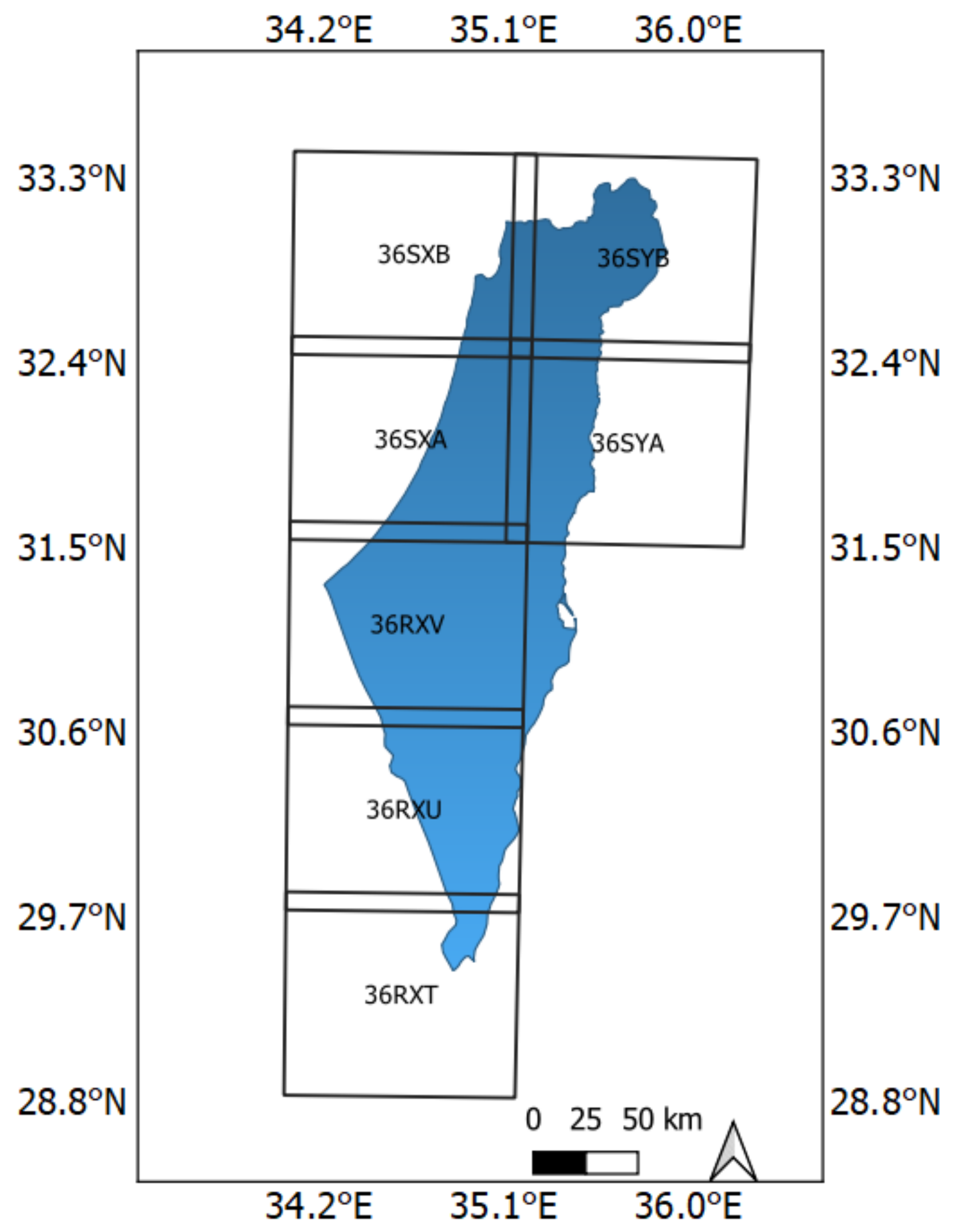
Figure 1. Sentinel-2 tiles over Israel.
Remotesensing 13 03488 g001
Figure 2. The workflow of the crop classification methodology.
Remotesensing 13 03488 g002
Figure 3. Phenology features. The x-axis value of the left red dot represents the SOS date, and the y-axis value of the left red dot represents the SOS VI value. The x-axis value of the right red dot represents the EOS date, and the y-axis value of the right red dot represents the EOS VI value. The x-axis value of the green dot represents the maximum date, and the y-axis value of the red dot represents the maximum VI value. The orange, green, and blue lines represent the growing season length, the length of the enhancement period, and the length of the reduction period, respectively.
Remotesensing 13 03488 g003
Figure 4. Train and test dataset distribution for each crop.
Remotesensing 13 03488 g004
Figure 5. IoU results of six parameters and input combinations (detailed in Table 1) applied to the mean shift segmentation algorithm. The box represents 50% of the data, from the 25th percentile to the 75th percentile. The horizontal line inside the box represents the median of the data. The lines extending from the box (whiskers) represent the lower or upper quartiles. The gray lines represent the standard deviation, and the gray squares represent the average of each combination.
Remotesensing 13 03488 g005
Figure 6. Segmentation output with mean shift algorithm using the green, red, and NIR bands as input and high emphasis on the spectral and spatial characteristics. (A) Segmented image of part of the study area. (B) Under segmentation problem. (C) Over segmentation problem.
Remotesensing 13 03488 g006
Figure 7. The number of output segments in part of the study area created using the mean shift algorithm and each one of the combinations (detailed in Table 1).
Remotesensing 13 03488 g007
Figure 8. An example of mean shift segmentation output using the blue, red, and NIR bands as input and high/low spectral and spatial parameters. (A) Input image (the green, red, and NIR bands). (B) Segmentation output using high emphasis on the spectral characteristic and low emphasis on the spatial characteristic (Combination 2). (C) Segmentation output using low emphasis on the spectral characteristic and high emphasis on the spatial characteristic (Combination 3). (D) Segmentation output using high emphasis on the spectral and spatial characteristics (Combination 1).
Remotesensing 13 03488 g008
Figure 9. The mean standard score of each crop for each one of the features. The error bars represent the confidence interval. Max date, EOS date, SOS date, Max NDII, EOS NDII, and SOS DNII refer to the dates when NDII value was at the maximum, the date when the growing season had started, the date when the growing season had ended, and the corresponding NDII values at theses dates, respectively. Length references the length of the growing season. Integral references the seasonal integral. Enhancement and Reduction refer to the enhancement and reduction periods.
Remotesensing 13 03488 g009
Figure 10. Feature importance for XGBoost and RF classifiers. The error bars represent the confidence interval for the four VIs (NDVI, OSAVI, NDRE, and NDII).
Remotesensing 13 03488 g010
Figure 11. Final object-based NDII time series XGBoost classification results in a part of the study area.
Remotesensing 13 03488 g011
Table 1. Characteristics importance (spectral and spatial) and input (image bands or VI) combinations tested using mean shift segmentation.
Combination
Number
Input Bands\IndexSpectral Characteristic
Importance
Spatial
Characteristic Importance
1Green, Red, NIRHigh (18)High (18)
2Green, Red, NIRHigh (18)Low (6)
3Green, Red, NIRLow (6)High (18)
4NDVIHigh (18)High (18)
5NDVIHigh (18)Low (6)
6NDVILow (6)High (18)
Table 2. OA and AUC results of the different classification methods.
OA (%) AUC (%)
AlgorithmVITrainValidationCross ValidationTrainValidationCross Validation
RFNDVI766664958786
OSAVI726564938586
NDRE827067968787
NDII766669968787
SVMNDVI726558918079
OSAVI726159917979
NDRE686263898182
NDII746663928282
XGBoostNDVI726765938686
OSAVI746565938484
NDRE786966958887
NDII756868958888
Table 3. UA and PA values of the different classification methods.
UA (%) PA (%)
CarrotCottonBarleyWheatChickpeaCarrotCottonBarleyWheatChickpea
RFNDVI60736467632170438955
OSAVI50676068631961468854
NDRE58746073672661448777
NDII58485672611748419163
SVMNDVI50654868711974418657
OSAVI57544067651957398157
NDRE54495467611770358455
NDII56474673712161448757
XGBoostNDVI60706769612170488759
OSAVI61716768552652418759
NDRE67636273662965528475
NDII82525571692148449066
Average 59615770642161438761
Table 4. Confusion matrix and validation results for NDII time series and XGBoost classifier.
Actual
CarrotCottonBarleyWheatChickpeaTotal # of
Classified Samples
User’s Accuracy %
Correct
PredictedCarrot902311560
Cotton2160232370
Barley4026723967
Wheat253211441721069
Chickpea24510335461
Total # of reference data samples42235416656
Producer’s accuracy % correct2170488759 OA = 68
Table 5. A number of OA results of crop classification from studies from the last decade.
Number of ClassesCrop TypeAreaObject/Pixel-BasedSatelliteClassifierAccuracyReference
4Cotton, spring maize, winter wheat and summer maize, tree.China,
5710 km2
Pixel-basedLandsat and Sentinel-2Artificial Immune NetworkOA: 97%[19]
8Citrus, sugar beet, fallow, cereals, urban, pomegranate, olive, alfalfa.Morocco, 970 km2Pixel-basedSentinel-2ARFOA: 88%[68]
8Rice, corn, water, soybean, potato, beet, building, forest.China, 3685 km2Pixel-basedSentinel-2RFOA: 97.8%[69]
SVMOA: 97.2%
Decision TreeOA: 95.9%
6Winter cereal, maize, soybean, winter rapeseed, sunflower.Ukraine
1184km2
Pixel-basedLandsat 8 and Sentinel-1SVM + RF fusionOA: 88%[36]
SVMOA: 75%
RFOA: 81.4%
6Been, beet root, grass, maize, potato, wheatJapan, over 200 km2Pixel-basedSentinel-2SVMOA: 90.6%[23]
RFOA: 89%
Ensemble machine learning methodOA: 91.6%
16Barley (spring + winter), beet, linseed, maize, wheat (spring + winter), potato, oats, oilseed, fallow, field beans (spring + winter), peas, grassland (permanent + temporary)UK,
400 km2
Object-basedWorldView-3, Sentinel-2RF and Decision Tree fusionOA: 91%[22]
4Soy, cotton, maize, othersBrazil, over 90,000 km2Pixel-basedMODISDecision TreeOA: 86%[33]
3Corn and soybean, others.United States,
2585 km2
Object-basedLandsat 5/7/8Machine learning model based on deep neural networkOA: 96%[10]
6Wheat, maize, rice, sunflower, forest, water.Romania, 638.77 km2Pixel-basedSentinel-2RFOA: 97%
[6]
Time-Weighted Dynamic Time WarpingOA: 95%
Object-basedRFOA: 98%
Time-Weighted Dynamic Time WarpingOA: 96%
6Forage, forest, maize, water, cereal, double cropping.Italy, 242.56 km2Pixel-basedRFOA: 87%
Time-Weighted Dynamic Time WarpingOA: 87%
Object-basedRFOA: 86%
Time-Weighted Dynamic Time WarpingOA: 90%
7Wheat, alfalfa, hay, sugar beets, onions, fallow, lettuce.California, USA 588.9 km2Pixel-basedRFOA: 89%
Time-Weighted Dynamic Time WarpingOA: 75%
Object-basedRFOA: 88%
Time-Weighted Dynamic Time WarpingOA: 78%
12Wheat, barley, rapeseed, maize, potatoes, beets, flax, grassland, forest, built-up, water, otherBelgium, 13,414.87 km2Pixel-basedSentinel-1 and Sentinel-2Hierarchical RFOA: 82%[70]
7Carrots, maize, onions, soya, sugar beet, sunflower, winter cropsAustria, 600 km2Pixel-basedSentinel-2RFOA: 83%[31]
Object-basedOA: 77%
9Alfalfa, cotton, corn, wheat, barley, potatoes barley-cotton, wheat-sorghum, and wheat-cottonArizona, USA,
1338 km2
Pixel-basedLandsat 5/7SVMOA: 90%[18]
10First crop corn, second crop corn, well-developed cotton, moderately developed cotton, weakly developed cotton, wet soil, moist soil, dry soil, and water surfaceTurkey, 17.3 km2Pixel-basedRapidEyeSVMOA: 87%[27]
3Cereal, pulse, otherMontana, USA, approximately 13,778 km2Object-basedLandsat ETM+RFOA: 85%[35]
Pixel-basedOA: 85%
6Cotton, fallow, other crops, pasture, sorghum, woodyAustralia, 1.7 million km2Object-basedLandsat TMSVMOA: 78%[34]
5Soybean, soybean + noncommercial crop, soybean + maize, soybean + cotton, cotton.Brazil, 906000 km2Pixel-based classification and object-based post-classificationMODISMaximum LikelihoodOA: 74%[71]
13Alfalfa, vineyard, almond, walnut, corn, rice, safflower, sunflower, tomato, oat, rye, wheat and meadow.California, USA, 2649 km2Object-basedASTERDecision TreeOA: 79%[8]
5Wheat, cotton, chickpea, barley, carrot.Israel, approximately 220 km2Object-basedSentinel-2FROA: 69%This study
SVMOA: 63%
XGBoostOA: 68%
Publisher’s Note: MDPI stays neutral with regard to jurisdictional claims in published maps and institutional affiliations.