Article

Surrogate Models Applied to Optimized Organic Rankine Cycles

by
Icaro Figueiredo Vilasboas
1,*,
Victor Gabriel Sousa Fagundes dos Santos
2,
Armando Sá Ribeiro, Jr.
3 and
Julio Augusto Mendes da Silva
4
1
Industrial Engineering Program (PEI), Federal University of Bahia, Salvador 40210-630, Brazil
2
Department of Electrical and Computer Engineering (DEEC), Federal University of Bahia, Salvador 40210-630, Brazil
3
Department of Construction and Structures (DCE), Federal University of Bahia, Salvador 40210-630, Brazil
4
Department of Mechanical Engineering (DEM), Federal University of Bahia, Salvador 40210-630, Brazil
*
Author to whom correspondence should be addressed.
Energies 2021, 14(24), 8456; https://doi.org/10.3390/en14248456
Submission received: 17 November 2021 / Revised: 6 December 2021 / Accepted: 9 December 2021 / Published: 15 December 2021

Abstract

:
Global optimization of industrial plant configurations using organic Rankine cycles (ORC) to recover heat is becoming attractive nowadays. This kind of optimization requires structural and parametric decisions to be made; the number of variables is usually high, and some of them generate disruptive responses. Surrogate models can be developed to replace the main components of the complex models reducing the computational requirements. This paper aims to create, evaluate, and compare surrogates built to replace a complex thermodynamic-economic code used to indicate the specific cost (US$/kWe) and efficiency of optimized ORCs. The ORCs are optimized under different heat sources conditions in respect to their operational state, configuration, working fluid and thermal fluid, aiming at a minimal specific cost. The costs of 1449.05, 1045.24, and 638.80 US$/kWe and energy efficiencies of 11.1%, 10.9%, and 10.4% were found for 100, 1000, and 50,000 kWt of heat transfer rate at average temperature of 345 °C. The R-square varied from 0.96 to 0.99 while the number of results with error lower than 5% varied from 88% to 75% depending on the surrogate model (random forest or polynomial regression) and output (specific cost or efficiency). The computational time was reduced in more than 99.9% for all surrogates indicated.

1. Introduction

Energy, environmental, and economic issues have guided researchers into the optimization of available energy sources. The use of waste heat and low temperature renewable sources to generate electricity using organic Rankine cycles (ORCs) has gained attention in the last decade. However, the use of organic substances as working fluid in power cycles emerged in the mid-1820s when Thomas Howard replaced water with ether in a power machine [1]. Since then, several works have reported the use organic fluids in Rankine cycles and highlighted the contributions of Luigi d’Amelio, who developed an experimental turbine using ethyl chloride in 1954, and Harry Zvi Tabor and Lucien Bronicki, whom tested small solar ORC units (2 kWe and 10 kWe) with monochlorobenzene in 1961 [2,3,4].
Over the years ORC systems have demonstrated some important advantages when compared to conventional power generation technologies including: (1) lower operational pressure; (2) supercritical cycles at lower temperature and pressure; (3) the possibility of selecting positive condensing pressure; (4) the possibility of selecting a fluid appropriated to the thermal source available; (5) efficient systems at small sizes; and (6) simpler cycle configurations [5]. Due to the good features reported, the commercial use of ORCs is now available worldwide. ORMAT (1964) and Turboden (1970) established themselves as pioneers in the ORC market and remain until now as big players in this field. However, other companies can also be highlighted such as Exergy, Turbine Air Systems (TAS), General Electric, Kaishan, Adoratec, among others. The total installed capacity of this technology at the end of 2016 was 2701 MW, mainly applied to geothermal sources, which represents 74.8% of the ORC installed capacity [6,7].
Currently, organic Rankine cycles (ORC) still represent a promising alternative to generate power from low and moderate temperatures [8,9]. In recent years, works have reported ORC systems using various thermal sources such as geothermal [10,11,12], biomass [13,14,15], solar thermal [16,17,18,19], and waste heat [20,21,22,23]. Optimization of ORC configuration, operating condition, and fluid selection for different applications are extensively reported in the literature and the objective function and heat source characteristics strongly affect the results obtained.
Astolfi et al. [24] and da Silva et al. [25] proposed an optimization based on the maximum power output of ORCs applied to geothermal sources (from 120 °C to 180 °C) and to a diesel engine flue gas (231 °C), respectively. Both concluded that the supercritical recuperative configuration is the most adequate for the different fluids analyzed. Wang et al. [26], Li et al. [27] and Mazetto et al. [28] optimized ORCs based on the maximization of power and minimization of heat exchanger area (i.e., power to area ratio), considering the total area of the heat exchangers as representative of investment cost. The authors presented the best working fluids at each specific applications: R123 and R141b to exhaust gas at temperatures between 100 °C and 220 °C [26]; R114 and R245fa to flue gas at 160 °C [27]; and R134a and R717 to recover heat from a hot diesel stream (140 °C) in a refinery [28].
Astolfi et al. [24] drew attention to the increase in the area of heat exchangers in supercritical and recuperative cycles and the importance of evaluating cost indicators; in [29], the same authors used total cost per power (€/kWe) to optimize an ORC for a geothermal source with temperatures between 120 °C and 180 °C. The authors concluded that the supercritical configuration provides the best performance from the thermodynamic-economic point of view. Garg e Orosz [18], on the other hand, used the specific cost divided by heat transfer effectiveness as an objective function for thermal sources with temperatures between 75 °C and 275 °C and installed capacity of 5 kWe, 50 kWe, and 500 kWe. Pure fluids and mixtures were evaluated and R134a and R152a were the best choices for all scenarios.
Feng et al. [30] and Song et al. [31] used a multi-objective optimization to maximize the exergy efficiency and minimize both payback time and levelized cost of energy (LCOE). They concluded that recuperative ORCs perform better than non-recuperative ORCs for the application reported (i.e., pressurized air at 150 °C and 5 bar). Song et al. [31], in turn, indicated a significant decrease in payback period when a supercritical ORC was selected in comparison to a subcritical ORC for a geothermal source at 180 °C.
The simultaneous thermodynamic-economic optimization of ORCs within broader systems such as optimizations involving heliothermic power plants, cogeneration plants and integration among chemical or industrial plants and ORCs can be expensive in computational terms. For these applications, surrogates, metamodels or response surface models can be used to replace the complex thermodynamic-economic codes by simpler and faster functions [32] relating the objective with the decision variables of the optimization problem [33,34,35,36]. The literature on the application of surrogate models in optimized power plant structure and operation is still scarce.
Rashidi et al. [37] performed three distinct optimizations to determine the maximum energy efficiency, exergy efficiency and specific power output of a supercritical recuperative ORC based on an artificial neural network (ANN) response surface. Luo et al. [38] optimized a heliothermic plant based on 12 decision variables, aiming at minimization of the LCOE, using the System Advisor Model (SAM) [39]. The relation between input variables and LCOE were approximated by a fourth-order function. De Araujo [40] applied surrogate models to represent the specific cost of a ORC, a Kalina cycle and a conventional Rankine cycle in a superstructure used to recover the waste heat from an internal combustion engine. Kazemian and Gandjalikhan Nassab [41] used a second order auxiliary function as surrogate to determine operating and design parameters for a gas turbine optimized in terms of efficiency and power.
This paper presents a comprehensive thermodynamic-economic optimization of structure, operating condition, working fluid and thermal oil for ORCs using heat sources from 100 kWt to 50 MWt at 70 °C to 350 °C. Two surrogate models are used to replace the thermodynamic-economic code in order to obtain quicker predictions for the optimized specific cost and efficiency. Thus, the novelty of this paper relies on:
  • Appling surrogate techniques to replace an entire optimization model instead of part of it as usually reported in the literature;
  • Evaluating the effect of different inputs used to represent heat source characteristics on the surrogates;
  • Making a comparison between stochastic and deterministic surrogates.

2. Methodology

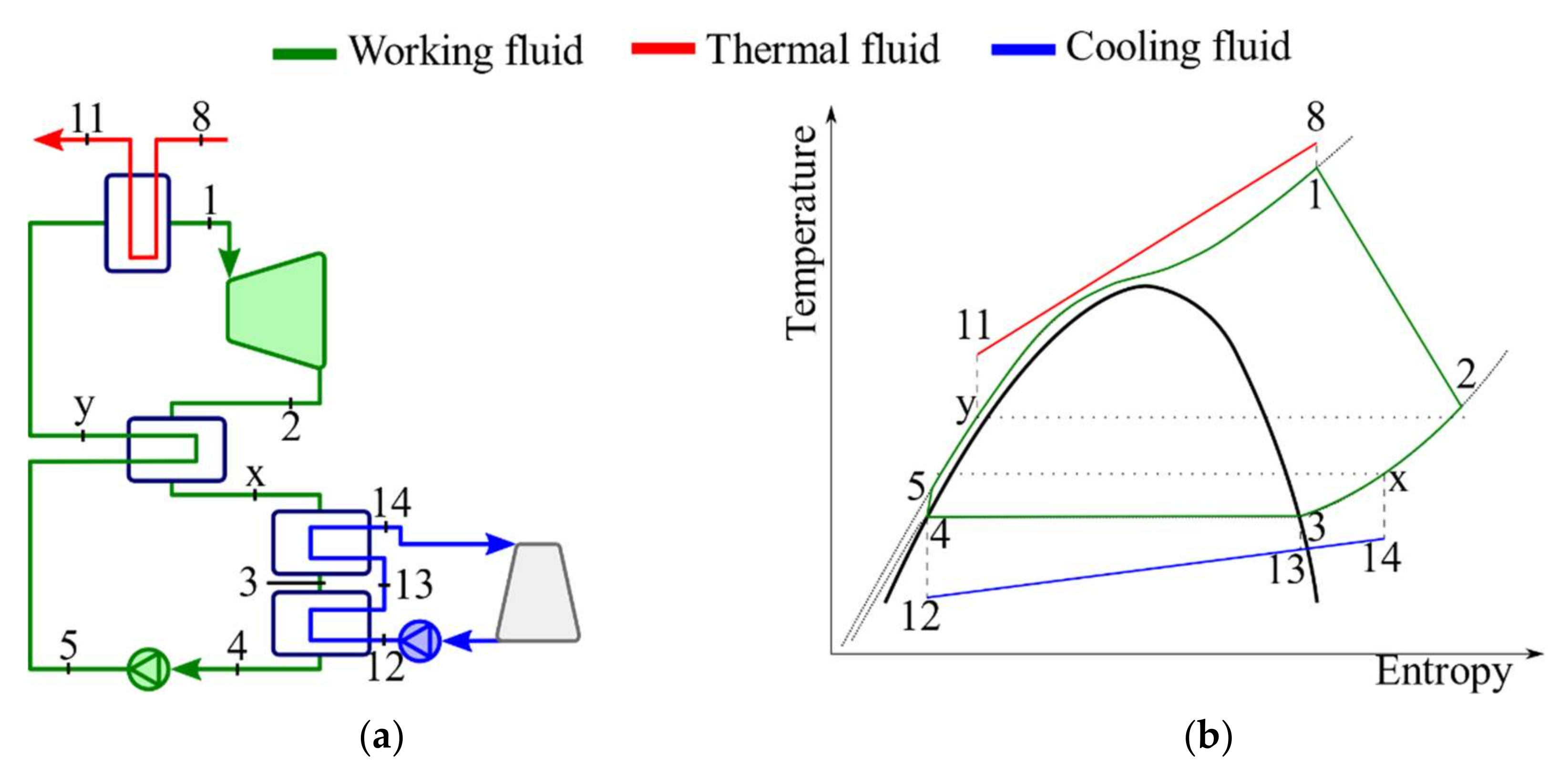
The thermodynamic-economic model can choose between subcritical, Figure 1, and supercritical configuration, Figure 2, with or without recuperation. The working fluid is indicated in green, thermal fluid (i.e., heat source) in red, and cooling water is represented in blue. These four configurations were named: subcritical or basic ORC (BORC), supercritical ORC (SORC), basic recuperative ORC (BRORC) and supercritical recuperative ORC (SRORC).
Six working fluids are tested based on the commercial ORCs fluids available on market [6,42]. Their main environmental and safety indicators are summarized in Table 1.
Syltherm 800 and Dowtherm A are selected as thermal fluids as they are widely used in solar thermal systems [43] and as ORC intermediary heat transfer fluid [44], both considered stable up to 400 °C and with melting point at −40 and 12 °C, respectively. As the heat exchanger used to heat the thermal fluid varies with the heat source characteristics, it was not considered in the thermodynamic-economic models.
The range of this application is defined by the inputs: (1) thermal fluid inlet temperature ( T 8 ), (2) thermal fluid outlet temperature ( T 11 ), and (3) heat transfer rate from the thermal fluid to working fluid ( Q ˙ 8 11 ) as indicated in Table 2.

2.1. Thermodynamic Model

The ORCs are modeled in steady state condition, potential and kinetic energy variations as well as energy loss to the environment from pipes and heat exchangers are neglected. Heat exchanges pressure drop, pinch point temperature difference and the minimum vapor quality during expansion are calculated and imposed as optimization constraints. Table 3 indicates the main parameters used for modeling the ORCs.
The isentropic efficiencies for the turbine ( η T , i s e ) and the pump ( η P , i s e ) are given in Equations (1) and (2), respectively, while energy balances for these components are given in Equations (3) and (4).
η T , i s e = h 1 h 2 h 1 h 2 , i s e
η P , i s e = h 5 , i s e h 4 h 5 h 4
W ˙ T = m ˙ w f h 1 h 2
W ˙ P = m ˙ w f h 5 h 4
Minimum quality of working fluid ( x T , m i n ) during expansion is verified dividing the turbine in ten small-stages and calculating the quality in each small-stage. The small-stages have constant polytropic efficiency ( η T ,   p o l y ) and pressure ratio ( p r T , s s ) as presented in Equation (5) [46]. Turbine reheat factor ( R H T ) measures the inefficiency of the complete expansion [46] and it is calculated using Equation (6) in which Δ h s s , i s e is the isentropic small-stage enthalpy difference.
η T , p o l y = η T , i s e R H T
R H T = Δ h s s , i s e h 1 h 2 , i s e
The energy balance for all heat exchangers is calculated based on Equation (7), in which the subscribe c is related to heat exchanger cold side, h to hot side, i n to heat exchanger inlet, and o u t to outlet.
m ˙ c h c , o u t h c , i n = m ˙ h h h , i n h h , o u t
Cooling tower energy balance, fan power consumption ( W ˙ C T ) and pressure variation ( Δ P C T ) are calculated according to the Equations (8)–(10) [47,48,49], respectively. The enthalpy of saturated air leaving the cooling tower ( h a i r , s a t , o u t ) is calculated at average cooling tower water temperature (45 °C) according to equation presented in Cortinovis et al. [48], while enthalpy ( h a i r , i n ) and density ( ρ a i r , i n ) of humid air are calculated as proposed by Pontes, Yamauchi, and Silva [49]. Cooling tower fill height ( Z ) is given in Equation (11) in which m ˙ c f ' is the cooling water mass flow rate and c p is the specific heat at the subscribed state. The integral at right-hand side of the Equation (11) is calculated based on Simpsons rule [47] and cooling tower mass transfer coefficient ( K a ) is described in Cortinovis et al. [48].
m ˙ c f h 14 h 12 = m a i r h a i r , s a t , o u t h a i r , i n
W ˙ C T = 1 + R h m a i r 2.98 ρ a i r , i n
Δ p C T = 10 5 3 + Z g ρ 12
Z K a m ˙ c f ' c p , 12 = T 12 T 14 d T h a i r , s a t h a i r
The rate in which heat is transferred from thermal fluid ( Q ˙ 8 11 ), the net electrical power ( W ˙ n e t ), and the cycle efficiency ( η O R C , e ) are given in Equations (12)–(14). The subscribe c f is related to the cooling fluid.
Q ˙ 8 11 = m ˙ h t f h 11 h 8
W ˙ n e t = η m η e W ˙ T W ˙ P + W ˙ P , c f + W ˙ F , c f η m η e
η O R C = W ˙ n e t Q ˙ 8 11
Finally, the input parameters used to characterize the heat source, Table 2 can be represented by exergy transfer rate, Equation (15), or using the rate of heat transfer ( Q ˙ 8 11 ) together with the average thermodynamic temperature ( T h t f , m e a n ), Equation (16), instead of T 8 and T 11 .
B ˙ = Q ˙ 8 11 1 T h t f , m e a n T 0
T h t f , m e a n = h 11 h 8 s 11 s 8

2.2. Plate Heat Exchangers Models

Plate heat exchangers (PHE) are commonly used in ORCs and were chosen due to their modular and compact format which usually provides high effectiveness [50,51] and low cost per area [52]. The rate in which heat is transferred from the thermal fluid to the working fluid, Equation (7), can also be written according to Equation (17).
Q ˙ = U A Δ T m e a n
The total heat exchanger area ( A ) is given in Equation (18) and the mean temperature difference ( Δ T m e a n ) is shown in Equation (19). In Equation (18) W is the plate width, L is the plate length and N p l is the number of plates.
A = W L ϕ N p l 2
Δ T m e a n = L M T D = Δ T i n Δ T o u t ln Δ T i n Δ T o u t
The overall heat transfer coefficient ( U ) depends on the thermal resistances and can be calculated according to the Equation (20), in which t is the plate thickness, k p l is the plate conductivity, and h c is the convection coefficient at the subscribed side.
1 U = t k p l + 1 h c c + 1 h c h
Characterization of the convection coefficient depends on the phase of the fluid at each heat exchanger side, Table 4 summarizes the equations used in each case.
Plate heat exchanger pressure loss ( Δ p ), Equation (21), is calculated as a sum of friction pressure loss ( Δ p f r i c ), Equation (22), port pressure loss ( Δ p p o r t ), Equation (23), elevation pressure loss ( Δ p e l e ), Equation (24), and acceleration pressure loss ( Δ p a c e ), Equation (25). The first three components are present in all heat exchangers while acceleration pressure loss is applicable only when there is a change in fluid quality.
Δ p = Δ p f r i c + Δ p p o r t + Δ p e l e + Δ p a c e
Δ p f r i c = 2 G p l 2 N p a s f c L e f ρ D h
Δ p e l e = ρ g L e f
Δ p p o r t = 1.4 N p a s G p o r t 2 2 ρ
Δ p a c e = G p l 2 x i n x o u t 1 / ρ v 1 / ρ l
The equations used to calculate friction coefficient were divided in three cases depending on phase of the fluid: no phase change and supercritical state, condensation, and evaporation. Table 5 shows the equations used in each case.
Thermodynamic, heat transfer, and pressure loss models were implemented using a Python code. The thermophysical properties are obtained using REFPROP v.10 [58] and CoolProp [59] with the exception for the transport properties of Solkatherm (SES36) for which extended corresponding states [59] using propane as reference fluid [60,61] are used.

2.3. Economic Model

The economic model for all components is given in Equation (26) according to Bejan et al. [62]. The reference cost ( C r e f ), reference capacity ( X r e f ) and the exponent α were obtained using Thermoflex® [63]. In this equation, f p is a pressure factor, f m is the material factor, and X is the equipment capacity. The Chemical Engineering Plant Cost Index ( C E P C I ) used in the reference is the current value, and thus the ratio C E P C I r e f / C E P C I is equal to 1.
C = f p f m C r e f X X r e f α C E P C I C E P C I r e f
Plant total cost is defined according to Equation (27) in which N e q u i p is the number of ORC components.
C t o t = i = 1 N e q u i p C i

2.4. Thermodynamic-Economic Optimization

The minimization of total cost per installed capacity (i.e., specific cost) was chosen as the objective function as indicated in Equation (28). The optimization constraints are presented in Table 6.
min s c = C t o t W ˙ n e t
The decision variables and their lower and upper bounds are shown in Table 7. Decision variables p 2 , p 1 , T 1 e T y were chosen since they represent operational aspects affecting the pumps, turbine and cooling tower power as well as the heat exchangers areas. On the other hand, the decision variables W e v a p , W c o n d , W r e c , v e v a p , v c o n d , and v r e c are project parameters related to the ORC heat exchangers area and pressure loss.
ORC optimization was carried out using a jMetalPy [64] genetic algorithm (GA) with a stopping criterion of 3000 generations. The four configurations (i.e., BORC, BRORC, SORC, and SRORC) using six working fluids and two thermal fluids were optimized separately for each combination of input parameters.

2.5. Surrogates for Optimized ORCs

The results obtained by the optimization together with the respective inputs are used to create surrogate models for quicker evaluation of optimized ORC specific cost ( s c ) and efficiency ( η O R C ). The inputs and outputs used for training and validation of surrogate models are listed in Table 8.
Random forest (RF) [65,66] and the polynomial regression (PR) [67] were selected as surrogate algorithms, which correspond to a non-parametric and a parametric method [68], respectively. Both are implemented in scikit-learn [69], a python module for predictive data analysis. In the case of PR surrogate, min-max-scaler [70] and power transformer [71] were required to normalize each input. The RF, on the other hand, did not require any transformation. Cross-validation [72] was applied with ten subsets of input/output for estimation of model performance.

3. Results and Discussion

3.1. Thermodynamic-Economic Optimization

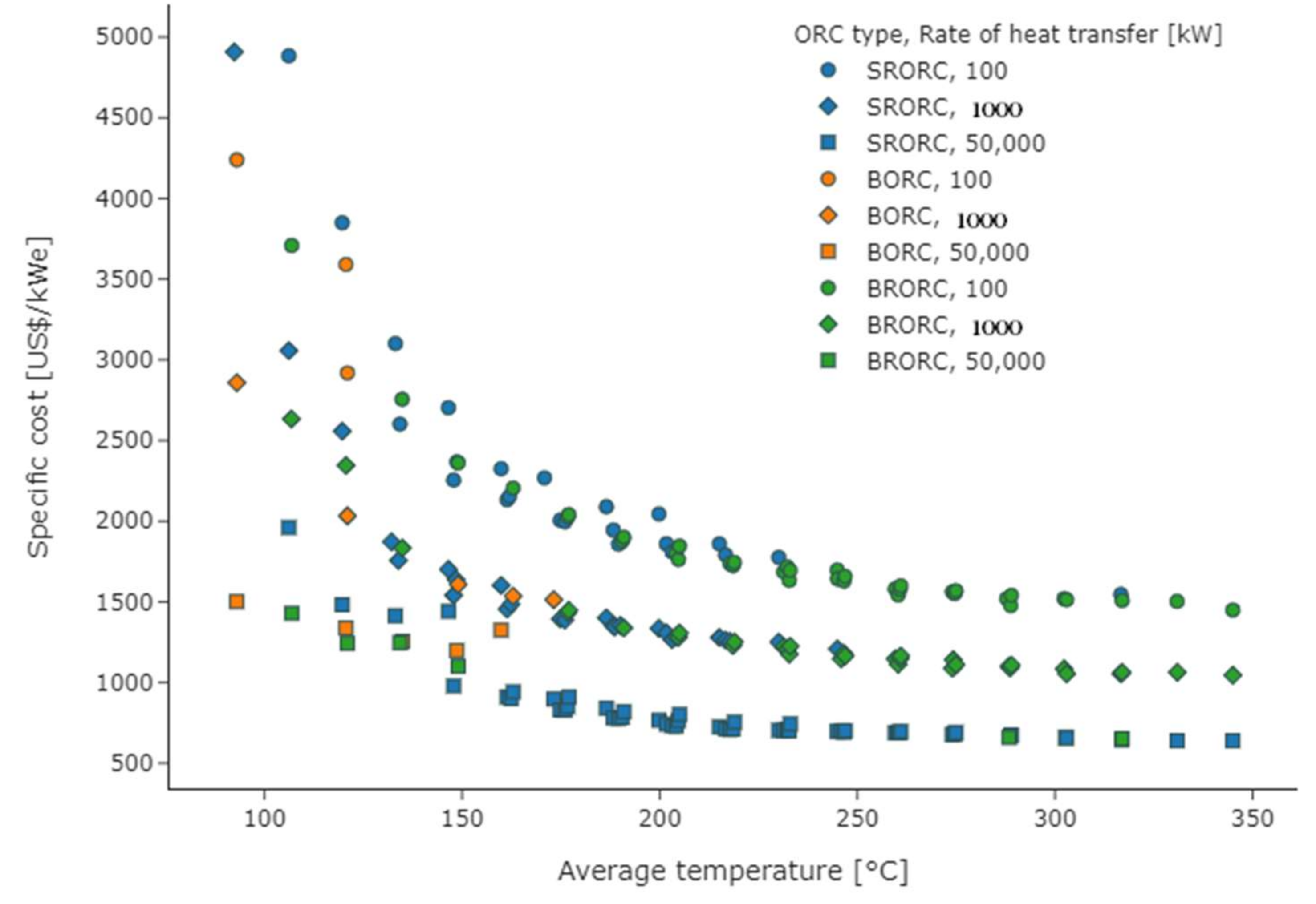
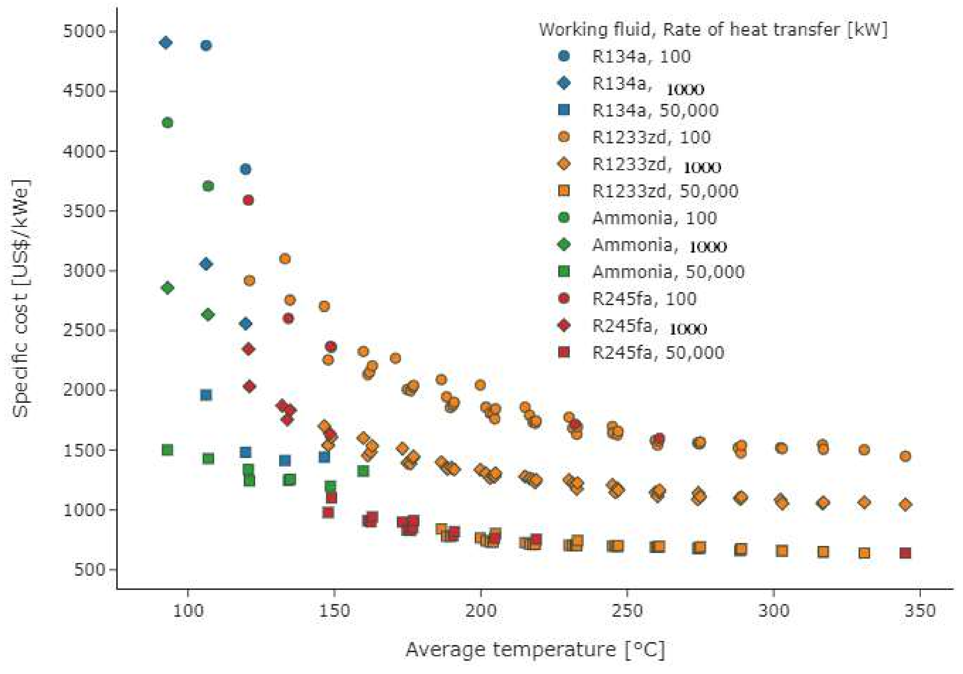
Figure 3 and Figure 4 show the ORCs minimum specific costs as function of heat source average temperature for three cases of heat transfer rate (100, 1000, and 50,000 kWt). While Figure 3 indicates the ORCs configurations, Figure 4 indicates their working fluids.
It is possible to observe that the ORCs specific costs decrease with the increase in the heat transfer rate due to reduction in the specific costs of equipment. The ORCs specific costs also decrease with the increase in the average temperature in which the heat is transferred due to the increase in the cycle efficiency. The minimum specific costs found were 1449.05, 1045.24, and 638.80 US$/kWe with energy efficiency of 11.1%, 10.9%, and 10.4% at the maximum average temperature of 345 °C. For the minimum average temperature of 93 °C, the specific costs were 4238.45, 2857.46, and 1501.09 US$/kWe with energy efficiency of about 2.5% for all cases at heat transfer rates of 100, 1000 and 50,000 kWt, respectively.
As shown in Figure 3, SRORC (blue) provides the lowest costs across most temperatures at 50,000 kWt, while BRORC (green) achieves the lowest values mainly at 100 and 1000 kWt. BORC (orange), on the other hand, provides low costs for the lower temperatures since there is almost no room for superheated vapor at both turbine inlet and outlet at these temperatures.
From Figure 4, it is possible to note that the isentropic fluids, R1233zd (orange) and R245fa (red), dominate the applications at higher temperatures while wet fluids, R134a (blue) and ammonia (green), are the most reasonable fluids for the lower temperature region which agrees with their lower critical temperatures (Table 1). It is also important to stress that working fluid selection is more dependent on temperature than on heat transfer rate. Different fluid selection for different heat transfer rates at same temperature is possible, however. It may occur since the overall heat transfer coefficient may play a significant role as the heat exchangers specific cost (USD/m2) changes with size.

3.2. Surrogates for Optimized ORCs

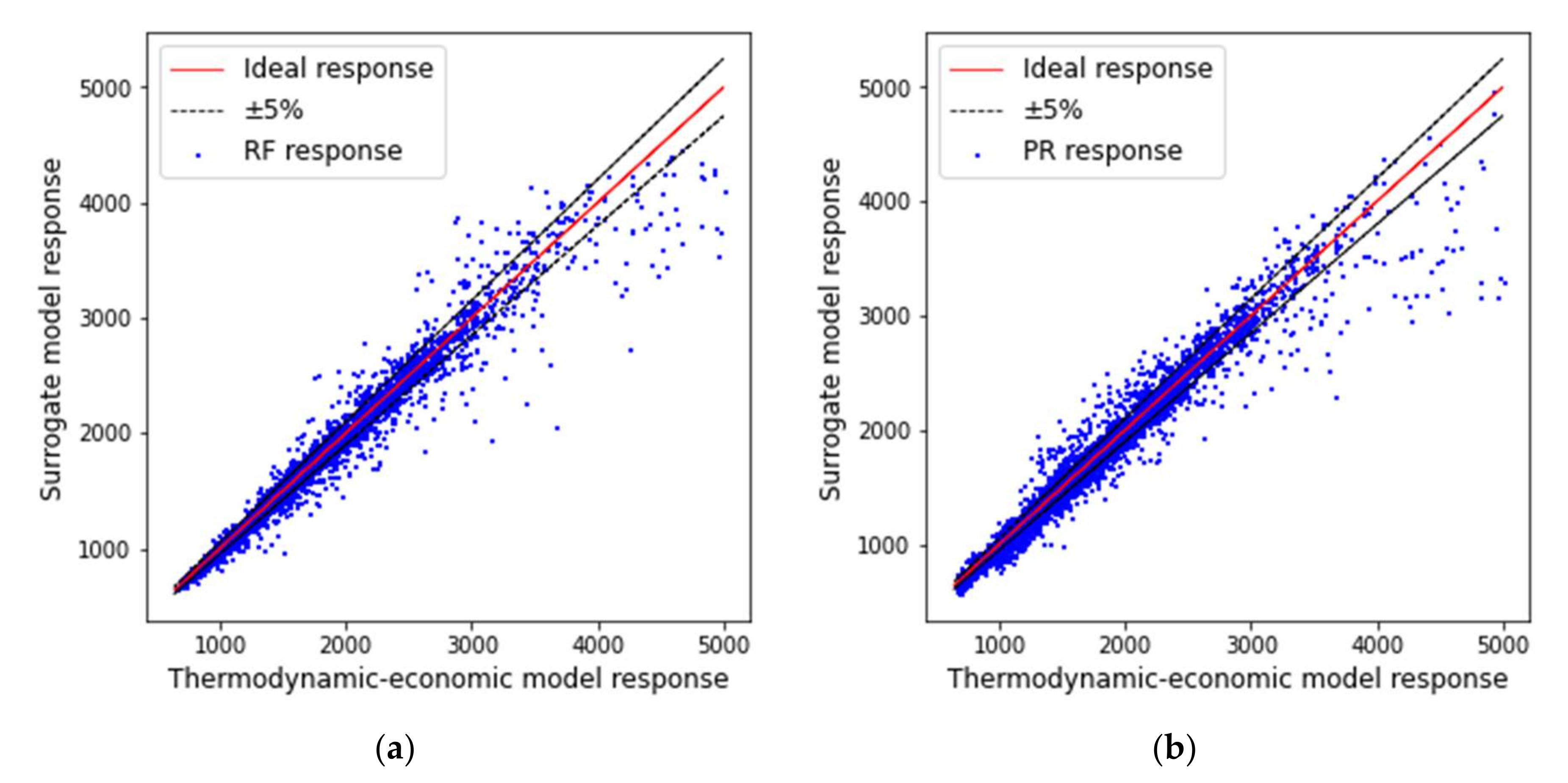
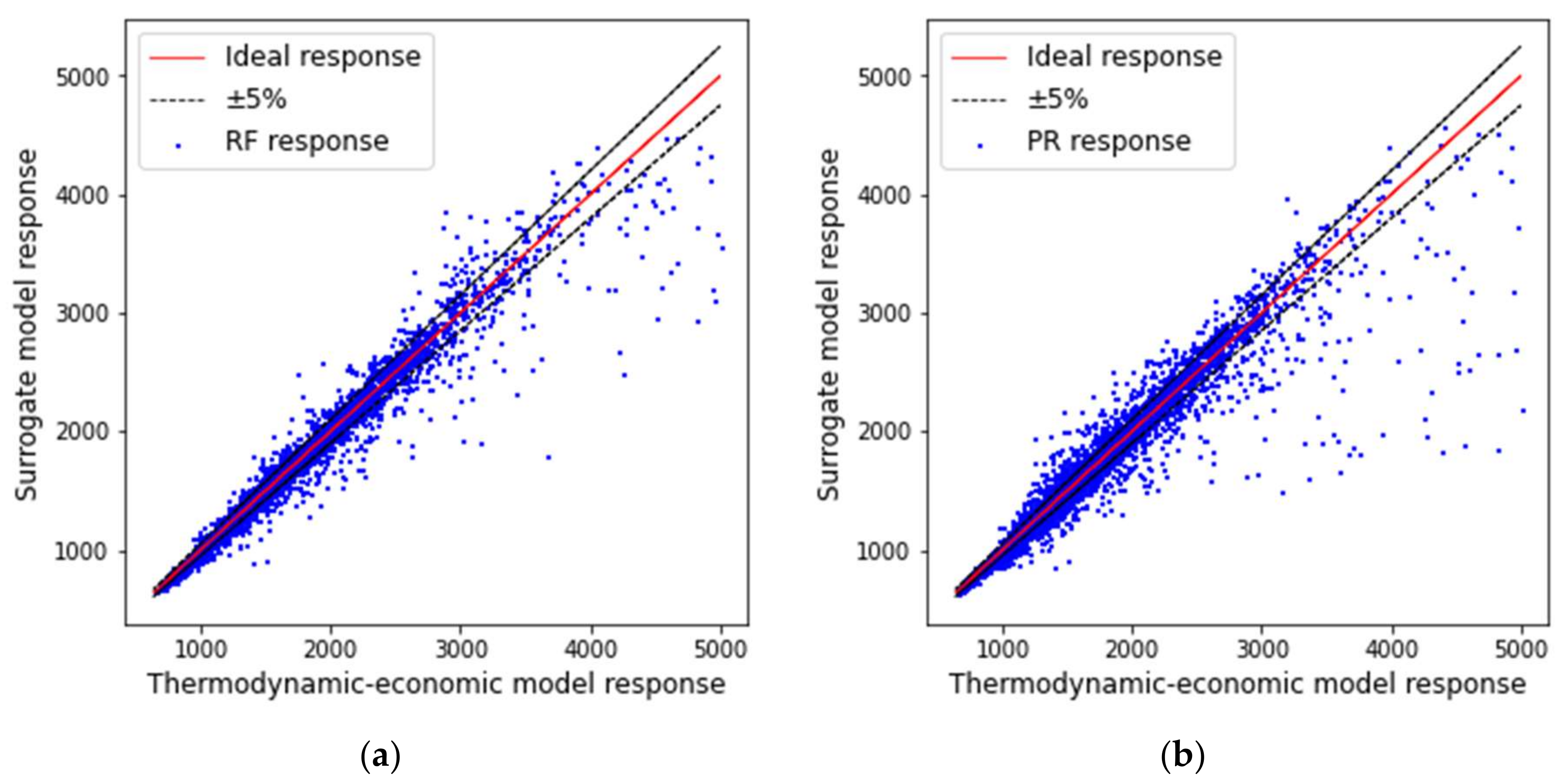
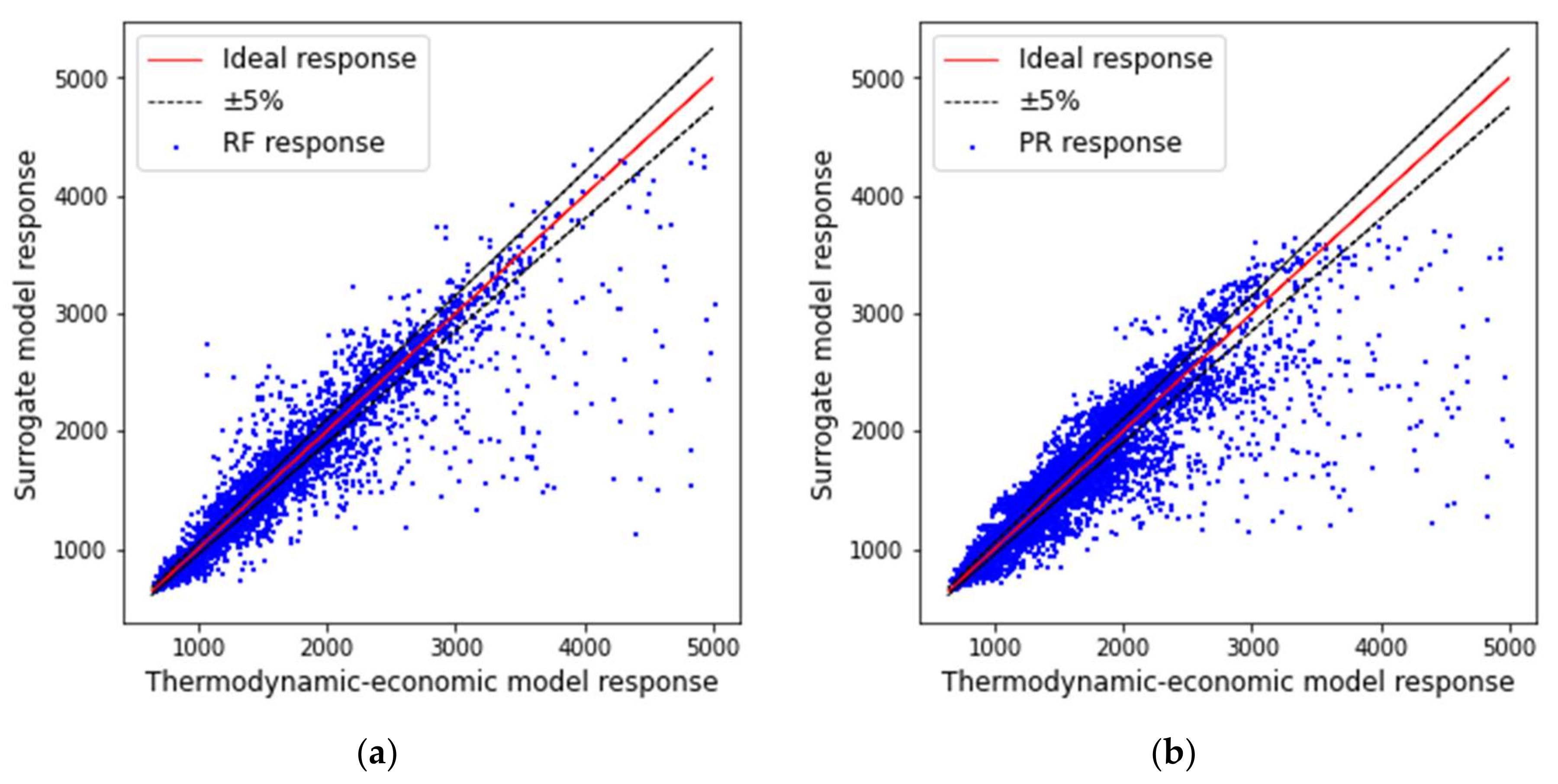
Surrogate and thermodynamic-economic models responses for the specific cost were assessed for three input groups representing the same thermodynamic condition: (1) heat input and output temperature ( T 8 and T 11 ) and heat transfer rate ( Q ˙ 8 11 ) ; (2) average temperature of heat transfer ( T h , m e a n ) and heat transfer rate ( Q ˙ 8 11 ); and (3) exergy transfer rate ( B ˙ ), Figure 5, Figure 6 and Figure 7, respectively. This comparison aims to evaluate the surrogate error as heat source condition is represented by a different number of inputs. Furthermore, heuristic (random forest regression, RF) and deterministic (polynomial regression, PR) surrogates were also assessed so that different search codes can be contemplated.
It is clear from Figure 5, Figure 6 and Figure 7 that some information is lost as the number of inputs decreases even though the heat source capacity to generate work can be represented by the three input groups. This lost information is related the sensibility of specific cost to temperatures and heat transfer rate in a magnitude different from that of exergy calculation.
Table 9 shows that random forest surrogate performs slightly better than polynomial regression for all cases. This can be explained by the presence of many discontinuities during optimization (e.g., the presence or not of recuperator, working fluid type and ORC configuration). These discontinuities are better represented by heuristic models than by deterministic ones. Additionally, as the ORCs were optimized to provide the lowest specific cost, a weaker adherence is found for ORC efficiency. Nevertheless, the results indicate that surrogates can replace complex thermodynamic-economic models in broader optimization codes using deterministic or heuristic search methods. The errors that arise from these simplified representations must be properly analyzed. Although high R-squares are obtained (0.96–0.99), the number of cases with error lower than 5% can be as low as 75% depending on the surrogate, which may be prohibitive in some applications.
Finally, the use of surrogates resulted in a significant reduction in processing time. While the thermodynamic-economic optimization requires around 723.2359 s to provide the efficiency and specific cost for a single application, RF and PR surrogates require only 0.0309 s and 0.0843 s, respectively, in a i5-10400F (4.3 GHz, 6 cores, 12 threads).

4. Conclusions

A detailed thermodynamic-economic model for optimization of ORCs was developed. Fluid selection and operational optimization were carried out to minimize specific cost for four ORC configurations subjected to a wide range of heat sources.
Optimizations revealed that R1233zd and R245fa were usually selected as the best working fluids for higher average temperatures while SRORC and BRORC were selected as best configurations in these conditions. For thermal sources with lower average temperatures, ammonia and R134a fluids and BORC configuration presented the lowest specific costs in most cases. The minimized specific costs ranged from 4238.45 to 638.80 US$/kWe while the energy efficiency varied from 2.5 to 11.1% as the heat source conditions varied from 100 kWt at 93 °C to 50,000 kWt at 345 °C, respectively.
Even though exergy transfer rate perfectly represents the capacity to generate work of a given heat source, there is loss of information when temperatures and heat transfer rate are grouped in a single input. This grouping of properties produces a negative impact on surrogates capacity to mimic the thermodynamic-economic model, especially when the objective function is an economic indicator.
The surrogates employing heat transfer rate and thermal fluid inlet and outlet temperatures provided R-square from 0.96 to 0.99. However, deeper evaluation of the error reveals that only 81% and 75% of the results were within a 5% of error range for RF and PR, respectively, what maybe be prohibitive in some applications. On the other hand, the processing time has been significantly reduced with the use of surrogate (99.996% and 99.988% for RF and PR models, respectively). This reduction allows the use of this optimization approach within broader and more complex optimization codes.

Author Contributions

Conceptualization, I.F.V. and J.A.M.d.S.; methodology, I.F.V. and J.A.M.d.S.; software, I.F.V. and V.G.S.F.d.S.; validation, I.F.V.; formal analysis, I.F.V., V.G.S.F.d.S. and J.A.M.d.S.; investigation, I.F.V. and J.A.M.d.S.; resources, I.F.V. and J.A.M.d.S.; data curation, I.F.V. and V.G.S.F.d.S.; writing—original draft preparation, I.F.V.; writing—review and editing, I.F.V., V.G.S.F.d.S., A.S.R.J. and J.A.M.d.S.; supervision, A.S.R.J. and J.A.M.d.S.; project administration, A.S.R.J.; funding acquisition, A.S.R.J. and J.A.M.d.S. All authors have read and agreed to the published version of the manuscript.

Funding

This research was funded by Grupo Global Participações em Energia (GPE) grant number PD-06961-0011/2019.

Institutional Review Board Statement

Not applicable.

Informed Consent Statement

Not applicable.

Data Availability Statement

Not applicable.

Acknowledgments

The authors would like to thank Grupo Global Participações em Energia (GPE) for the financial support under Agência Nacional de Energia Elétrica (ANEEL) P&D program, project number PD-06961-0011/2019.

Conflicts of Interest

The authors declare no conflict of interest.

References

  1. Invernizzi, C.M. Closed Power Cycles. In Lecture Notes in Energy; Springer: London, UK, 2013; Volume 11, ISBN 978-1-4471-5139-5. [Google Scholar]
  2. Spencer, L. A comprehensive review of small solar-powered heat engines: Part I. A history of solar-powered devices up to 1950. Sol. Energy 1989, 43, 191–196. [Google Scholar] [CrossRef]
  3. Spencer, L. A comprehensive review of small solar-powered heat engines: Part II. Research since 1950—“conventional” engines up to 100 kW. Sol. Energy 1989, 43, 197–210. [Google Scholar] [CrossRef]
  4. Spencer, L. A comprehensive review of small solar-powered heat engines: Part III. Research since 1950—“unconventional” engines up to 100 kW. Sol. Energy 1989, 43, 211–225. [Google Scholar] [CrossRef]
  5. Babatunde, A.F.; Sunday, O.O. A Review of Working Fluids for Organic Rankine Cycle (ORC) Applications. IOP Conf. Series: Mater. Sci. Eng. 2018, 413, 012019. [Google Scholar] [CrossRef]
  6. Quoilin, S.; Broek, M.V.D.; Declaye, S.; Dewallef, P.; Lemort, V. Techno-economic survey of Organic Rankine Cycle (ORC) systems. Renew. Sustain. Energy Rev. 2013, 22, 168–186. [Google Scholar] [CrossRef] [Green Version]
  7. Tartière, T.; Astolfi, M. A World Overview of the Organic Rankine Cycle Market. Energy Procedia 2017, 129, 2–9. [Google Scholar] [CrossRef]
  8. Chen, H.; Goswami, D.Y.; Stefanakos, E.K. A review of thermodynamic cycles and working fluids for the conversion of low-grade heat. Renew. Sustain. Energy Rev. 2010, 14, 3059–3067. [Google Scholar] [CrossRef]
  9. Khennich, M.; Galanis, N. Optimal Design of ORC Systems with a Low-Temperature Heat Source. Entropy 2012, 14, 370–389. [Google Scholar] [CrossRef] [Green Version]
  10. Hettiarachchi, H.M.; Golubovic, M.; Worek, W.M.; Ikegami, Y. Optimum design criteria for an Organic Rankine cycle using low-temperature geothermal heat sources. Energy 2007, 32, 1698–1706. [Google Scholar] [CrossRef]
  11. Shengjun, Z.; Huaixin, W.; Tao, G. Performance comparison and parametric optimization of subcritical Organic Rankine Cycle (ORC) and transcritical power cycle system for low-temperature geothermal power generation. Appl. Energy 2011, 88, 2740–2754. [Google Scholar] [CrossRef]
  12. Loni, R.; Mahian, O.; Najafi, G.; Sahin, A.Z.; Rajaee, F.; Kasaeian, A.; Mehrpooya, M.; Bellos, E.; le Roux, W.G. A critical review of power generation using geothermal-driven organic Rankine cycle. Therm. Sci. Eng. Prog. 2021, 25, 101028. [Google Scholar] [CrossRef]
  13. Drescher, U.; Brüggemann, D. Fluid selection for the Organic Rankine Cycle (ORC) in biomass power and heat plants. Appl. Therm. Eng. 2007, 27, 223–228. [Google Scholar] [CrossRef]
  14. Liu, H.; Shao, Y.; Li, J. A biomass-fired micro-scale CHP system with organic Rankine cycle (ORC)—Thermodynamic modelling studies. Biomass Bioenergy 2011, 35, 3985–3994. [Google Scholar] [CrossRef]
  15. Jang, Y.; Lee, J. Optimizations of the organic Rankine cycle-based domestic CHP using biomass fuel. Energy Convers. Manag. 2018, 160, 31–47. [Google Scholar] [CrossRef]
  16. Jing, L.; Gang, P.; Jie, J. Optimization of low temperature solar thermal electric generation with Organic Rankine Cycle in different areas. Appl. Energy 2010, 87, 3355–3365. [Google Scholar] [CrossRef]
  17. Quoilin, S.; Orosz, M.; Hemond, H.; Lemort, V. Performance and design optimization of a low-cost solar organic Rankine cycle for remote power generation. Sol. Energy 2011, 85, 955–966. [Google Scholar] [CrossRef] [Green Version]
  18. Garg, P.; Orosz, M.S. Economic optimization of Organic Rankine cycle with pure fluids and mixtures for waste heat and solar applications using particle swarm optimization method. Energy Convers. Manag. 2018, 165, 649–668. [Google Scholar] [CrossRef]
  19. Wu, D.; Zuo, J.; Liu, Z.; Han, Z.; Zhang, Y.; Wang, Q.; Li, P. Thermodynamic analyses and optimization of a novel CCHP system integrated organic Rankine cycle and solar thermal utilization. Energy Convers. Manag. 2019, 196, 453–466. [Google Scholar] [CrossRef]
  20. Vélez, F.; Segovia, J.J.; Martin, M.C.; Antolín, G.; Chejne, F.; Quijano, A. A technical, economical and market review of organic Rankine cycles for the conversion of low-grade heat for power generation. Renew. Sustain. Energy Rev. 2012, 16, 4175–4189. [Google Scholar] [CrossRef]
  21. Apostol, V.; Pop, H.; Dobrovicescu, A.; Prisecaru, T.; Alexandru, A.; Prisecaru, M. Thermodynamic Analysis of ORC Configurations Used for WHR from a Turbocharged Diesel Engine. Procedia Eng. 2015, 100, 549–558. [Google Scholar] [CrossRef] [Green Version]
  22. Akman, M.; Ergin, S. Thermo-environmental analysis and performance optimisation of transcritical organic Rankine cycle system for waste heat recovery of a marine diesel engine. Ships Offshore Struct. 2020, 16, 1104–1113. [Google Scholar] [CrossRef]
  23. Varshil, P.; Deshmukh, D. A comprehensive review of waste heat recovery from a diesel engine using organic rankine cycle. Energy Rep. 2021, 7, 3951–3970. [Google Scholar] [CrossRef]
  24. Astolfi, M.; Romano, M.C.; Bombarda, P.; Macchi, E. Binary ORC (organic Rankine cycles) power plants for the exploitation of medium–low temperature geothermal sources—Part A: Thermodynamic optimization. Energy 2014, 66, 423–434. [Google Scholar] [CrossRef]
  25. Da Silva, J.A.; Seifert, V.; de Morais, V.O.; Tsolakis, A.; Herreros, J.; Torres, E. Exergy evaluation and ORC use as an alternative for efficiency improvement in a CI-engine power plant. Sustain. Energy Technol. Assess. 2018, 30, 216–223. [Google Scholar] [CrossRef]
  26. Wang, Z.Q.; Zhou, N.J.; Guo, J.; Wang, X.Y. Fluid selection and parametric optimization of organic Rankine cycle using low temperature waste heat. Energy 2012, 40, 107–115. [Google Scholar] [CrossRef]
  27. Li, Y.-R.; Wang, J.-N.; Du, M.-T. Influence of coupled pinch point temperature difference and evaporation temperature on performance of organic Rankine cycle. Energy 2012, 42, 503–509. [Google Scholar] [CrossRef]
  28. Mazetto, B.M.; Da Silva, J.A.M.; Junior, S.D.O. Are ORCs a Good Option for Waste Heat Recovery in a Petroleum Refinery? Int. J. Thermodyn. 2015, 18, 161. [Google Scholar] [CrossRef] [Green Version]
  29. Astolfi, M.; Romano, M.C.; Bombarda, P.; Macchi, E. Binary ORC (Organic Rankine Cycles) power plants for the exploitation of medium–low temperature geothermal sources—Part B: Techno-economic optimization. Energy 2014, 66, 435–446. [Google Scholar] [CrossRef]
  30. Feng, Y.; Zhang, Y.; Li, B.; Yang, J.; Shi, Y. Comparison between regenerative organic Rankine cycle (RORC) and basic organic Rankine cycle (BORC) based on thermoeconomic multi-objective optimization considering exergy efficiency and levelized energy cost (LEC). Energy Convers. Manag. 2015, 96, 58–71. [Google Scholar] [CrossRef]
  31. Song, J.; Loo, P.; Teo, J.; Markides, C. Thermo-Economic Optimization of Organic Rankine Cycle (ORC) Systems for Geothermal Power Generation: A Comparative Study of System Configurations. Front. Energy Res. 2020, 8, 6. [Google Scholar] [CrossRef] [Green Version]
  32. Forrester, A.I.J.; Sóbester, A.; Keane, A.J. Engineering Design via Surrogate Modelling; John Wiley & Sons: Hoboken, NJ, USA, 2008; ISBN 9780470060681. [Google Scholar]
  33. Pires, T.S.; Cruz, M.E.; Colaço, M.J. Response surface method applied to the thermoeconomic optimization of a complex cogeneration system modeled in a process simulator. Energy 2013, 52, 44–54. [Google Scholar] [CrossRef]
  34. Riyanto, H.; Martowibowo, S.Y. Optimization of Organic Rankine Cycle Waste Heat Recovery for Power Generation in a Cement Plant via Response Surface Methodology. Int. J. Technol. 2015, 6, 938. [Google Scholar] [CrossRef]
  35. Zhang, X.S.; Yang, B.; Yu, T.; Jiang, L. Dynamic Surrogate Model Based Optimization for MPPT of Centralized Thermoelectric Generation Systems under Heterogeneous Temperature Difference. IEEE Trans. Energy Convers. 2020, 35, 966–976. [Google Scholar] [CrossRef]
  36. Kazemian, A.; Basati, Y.; Khatibi, M.; Ma, T. Performance prediction and optimization of a photovoltaic thermal system integrated with phase change material using response surface method. J. Clean. Prod. 2021, 290, 125748. [Google Scholar] [CrossRef]
  37. Rashidi, M.M.; Bég, O.A.; Parsa, A.B.; Nazari, F. Analysis and optimization of a transcritical power cycle with regenerator using artificial neural networks and genetic algorithms. Proc. Inst. Mech. Eng. Part A J. Power Energy 2011, 225, 701–717. [Google Scholar] [CrossRef]
  38. Luo, Y.; Hu, Y.; Lu, T. Efficient optimized design of solar power tower plants based on successive response surface methodology. Int. J. Low-Carbon Technol. 2019, 14, 475–486. [Google Scholar] [CrossRef]
  39. National Renewable Energy Laboratory System Advisor Model 2020. Available online: https://sam.nrel.gov/ (accessed on 1 October 2021).
  40. De Araújo, L.R. O uso do Método de Superfície de Resposta na Otimização Termoeconômica de Superestruturas Modeladas em Software Comercial para Projeto de Sistemas de Recuperação de Calor Residual em Motores Diesel Estacionários; Universidade Federal do Espírito Santo: Espírito Santo, Brazil, 2020. [Google Scholar]
  41. Kazemian, M.E.; Nassab, S.A.G. Thermodynamic Analysis and Statistical Investigation of Effective Parameters for Gas Turbine Cycle using the Response Surface Methodology. Int. J. Eng. 2020, 33, 894–905. [Google Scholar] [CrossRef]
  42. Dincer, I.; Zamfirescu, C. Conventional Power Generating Systems. In Advanced Power Generation Systems; Elsevier BV: Amsterdam, The Netherlands, 2014; pp. 199–310. [Google Scholar]
  43. Moens, L.; Blake, D.M. Advanced Heat Transfer and Thermal Storage Fluids. In Proceedings of the International Solar Energy Conference, Orlando, FL, USA, 6–12 August 2005; pp. 791–793. [Google Scholar]
  44. Jiménez-Arreola, M.; Wieland, C.; Romagnoli, A. Direct vs. indirect evaporation in Organic Rankine Cycle (ORC) systems: A comparison of the dynamic behavior for waste heat recovery of engine exhaust. Appl. Energy 2019, 242, 439–452. [Google Scholar] [CrossRef]
  45. Tascioni, R. Advanced Modeling of a Micro Solar CHP System for Residential Applications; Sapienza—University of Rome: Rome, Italy, 2021. [Google Scholar]
  46. Wang, T. The gas and steam turbines and combined cycle in IGCC systems. In Integrated Gasification Combined Cycle (IGCC) Technologies; Elsevier BV: Amsterdam, The Netherlands, 2017; pp. 497–640. ISBN 9780081001851. [Google Scholar]
  47. Leeper, S. Wet Cooling Towers—Rule-of-Thumb; U.S. Department of Energy: Washington, DC, USA, 1981. [Google Scholar]
  48. Cortinovis, G.F.; Ribeiro, M.T.; Paiva, J.L.; Song, T.W.; Pinto, J.M. Integrated analysis of cooling water systems: Modeling and experimental validation. Appl. Therm. Eng. 2009, 29, 3124–3131. [Google Scholar] [CrossRef]
  49. Pontes, R.F.; Yamauchi, W.M.; Silva, E.K. Analysis of the effect of seasonal climate changes on cooling tower efficiency, and strategies for reducing cooling tower power consumption. Appl. Therm. Eng. 2019, 161, 114148. [Google Scholar] [CrossRef]
  50. Kakaç, S.; Liu, H.; Pramuanjaroenkij, A. Heat Exchangers: Selection, Rating, and Thermal Design, 3rd ed.; CRC Press: Boca Raton, FL, USA, 2012; Volume 6, ISBN 1439849900. [Google Scholar]
  51. Yu, G.; Shu, G.; Tian, H.; Wei, H.; Liang, X. Multi-approach evaluations of a cascade-Organic Rankine Cycle (C-ORC) system driven by diesel engine waste heat: Part B-techno-economic evaluations. Energy Convers. Manag. 2016, 108, 596–608. [Google Scholar] [CrossRef]
  52. Lim, T.-W.; Choi, Y.-S.; Lee, C.-K. Design of plate heat exchangers for use in medium temperature organic Rankine cycles. Heat Mass Transf. 2018, 55, 165–174. [Google Scholar] [CrossRef]
  53. Martin, H. A theoretical approach to predict the performance of chevron-type plate heat exchangers. Chem. Eng. Process. Process. Intensif. 1996, 35, 301–310. [Google Scholar] [CrossRef]
  54. Kim, I.-K.; Park, J.-H.; Kwon, Y.-H.; Kim, Y.-S. Experimental Study on R-410a Evaporation Heat Transfer Characteristics in Oblong Shell and Plate Heat Exchanger. Heat Transf. Eng. 2007, 28, 633–639. [Google Scholar] [CrossRef]
  55. Yan, Y.-Y.; Lio, H.-C.; Lin, T.-F. Condensation heat transfer and pressure drop of refrigerant R-134a in a plate heat exchanger. Int. J. Heat Mass Transf. 1999, 42, 993–1006. [Google Scholar] [CrossRef]
  56. Karellas, S.; Schuster, A.; Leontaritis, A.-D. Influence of supercritical ORC parameters on plate heat exchanger design. Appl. Therm. Eng. 2012, 33-34, 70–76. [Google Scholar] [CrossRef]
  57. Huang, J.; Sheer, T.J.; Bailey-McEwan, M. Heat transfer and pressure drop in plate heat exchanger refrigerant evaporators. Int. J. Refrig. 2012, 35, 325–335. [Google Scholar] [CrossRef]
  58. Lemmon, E.W.; Bell, I.H.; Huber, M.L.; McLinden, M.O. NIST Standard Reference Database 23: Reference Fluid Thermodynamic and Transport Properties-REFPROP, version 10.0; National Institute of Standards and Technology: Gaithersburg, MD, USA, 2018. [Google Scholar]
  59. Bell, I.H.; Wronski, J.; Quoilin, S.; Lemort, V. Pure and Pseudo-pure Fluid Thermophysical Property Evaluation and the Open-Source Thermophysical Property Library CoolProp. Ind. Eng. Chem. Res. 2014, 53, 2498–2508. [Google Scholar] [CrossRef] [Green Version]
  60. Vogel, E.; Küchenmeister, C.; Bich, E.; Laesecke, A. Reference Correlation of the Viscosity of Propane. J. Phys. Chem. Ref. Data 1998, 27, 947–970. [Google Scholar] [CrossRef]
  61. Marsh, K.N.; Perkins, A.R.A.; Ramires, M.L.V. Measurement and Correlation of the Thermal Conductivity of Propane from 86 K to 600 K at Pressures to 70 MPa. J. Chem. Eng. Data 2002, 47, 932–940. [Google Scholar] [CrossRef]
  62. Bejan, A.; Tsatsaronis, G.; Moran, M. Thermal Design and Optimization, 1st ed.; John Wiley & Sons, Inc.: Hoboken, NJ, USA, 1995; ISBN 978-0-471-58467-4. [Google Scholar]
  63. Thermoflow Inc. Thermoflex; Thermoflow Inc.: Jacksonville, FL, USA, 2021. [Google Scholar]
  64. Benítez-Hidalgo, A.; Nebro, A.J.; García-Nieto, J.; Oregi, I.; Del Ser, J. jMetalPy: A Python framework for multi-objective optimization with metaheuristics. Swarm Evol. Comput. 2019, 51, 100598. [Google Scholar] [CrossRef] [Green Version]
  65. Breiman, L. Random Forests. Mach. Learn. 2001, 45, 5–32. [Google Scholar] [CrossRef] [Green Version]
  66. Geurts, P.; Ernst, D.; Wehenkel, L. Extremely randomized trees. Mach. Learn. 2006, 63, 3–42. [Google Scholar] [CrossRef] [Green Version]
  67. Ostertagová, E. Modelling using Polynomial Regression. Procedia Eng. 2012, 48, 500–506. [Google Scholar] [CrossRef] [Green Version]
  68. Queipo, N.V.; Haftka, R.T.; Shyy, W.; Goel, T.; Vaidyanathan, R.; Tucker, P.K. Surrogate-based analysis and optimization. Prog. Aerosp. Sci. 2005, 41, 1–28. [Google Scholar] [CrossRef] [Green Version]
  69. Pedregosa, F.; Varoquaux, G.; Gramfort, A.; Michel, V.; Thirion, B.; Grisel, O.; Blondel, M.; Prettenhofer, P.; Weiss, R.; Dubourg, V.; et al. Scikit-learn: Machine Learning in Python. J. Mach. Learn. Res. 2011, 12, 2825–2830. [Google Scholar] [CrossRef]
  70. Mustaffa, Z.; Yusof, Y. A Comparison of Normalization Techniques in Predicting Dengue Outbreak. Int. Conf. Bus. Econ. Res. 2010, 1, 345–349. [Google Scholar]
  71. Raymaekers, J.; Rousseeuw, P.J. Transforming variables to central normality. Mach. Learn. 2021, 1–23. [Google Scholar] [CrossRef]
  72. Kohavi, R. A Study of Cross-Validation and Bootstrap for Accuracy Estimation and Model Selection. Int. Jt. Conf. Artif. Intell. 1995, 14, 1137–1145. [Google Scholar]
Figure 1. Subcritical ORC (a) configuration and (b) T-s diagram.
Energies 14 08456 g001
Figure 2. Supercritical ORC (a) configuration and (b) T-s diagram.
Energies 14 08456 g002
Figure 3. ORC configurations for minimum specific costs.
Energies 14 08456 g003
Figure 4. ORC working fluids for minimum specific costs.
Energies 14 08456 g004
Figure 5. Thermodynamic-economic vs. surrogate model response using Q ˙ 8 11 , T 8 and T 11 as input to determine the minimal specific cost: (a) random forest regression and (b) polynomial regression.
Energies 14 08456 g005
Figure 6. Thermodynamic-economic vs. surrogate model response using Q ˙ 8 11 , and T h , m e a n as input to determine the minimal specific cost: (a) random forest regression and (b) polynomial regression.
Energies 14 08456 g006
Figure 7. Thermodynamic-economic vs. surrogate model response using B ˙ as input to determine the minimal specific cost: (a) random forest regression and (b) polynomial regression.
Energies 14 08456 g007
Table 1. Thermodynamic and environmental features of selected working fluids.
FluidMolecular FormulaTypeODPGWPSafety GroupEvaporation
Temperature 1
(°C)
Critical
Temperature
(°C)
Critical
Pressure
(bar)
D4 C 8 H 24 O 4 Si 4 Dry0-A2175.74313.3513.47
R134a C 2 H 2 F 4 Wet01370A1−26.07101.0640.59
R245fa C 3 H 3 F 5 Isentropic01050B115.05153.8636.51
Ammonia NH 3 Wet00B2−33.32132.25113.33
R1233zd C 3 H 2 ClF 3 Isentropic01A118.26166.4536.24
SES36 C 4 H 5 F 5 + CF CF 3 CF 2 O x CF 2 O y Dry03710A135.72177.5528.49
1 At 1 atm.
Table 2. Input lower and upper bounds.
Input ParameterLower BoundUpper Bound
T 8 60 °C340 °C
T 11 70 °C350 °C
Q ˙ 8 11 100 kWt50,000 kWt
Table 3. ORC thermodynamic parameters.
ParameterDescriptionValueReference
T 0 Ambient dry bulb temperature27.1 °C
p 0 Ambient pressure1.007 bar
R h Ambient relative humidity79.9%
η T , i s e Expander isentropic efficiency53%[45]
η P , i s e Pump isentropic efficiency70%[45]
η m Transmission efficiency95%[45]
η e Generator/motor efficiency90%[45]
T 12 Cooling fluid inlet temperature40 °C
T 14 Cooling fluid outlet temperature50 °C
Table 4. Convection coefficient equation for each phase of the working, thermal and cooling fluids.
ConditionEquationReference
No phase change h = 0.122 k D h Pr 1 / 3 f Re 2 sen 2 β 0.374 μ μ w 1 / 6 [53]
Evaporation h = 5.323 k D h Pr 1 / 3 Re e q 0.42 [54]
Condensation h = 4.118 k D h Pr 1 / 3 Re e q 0.42 [55]
Supercritical state h = 0.0183 k D h Pr 0.5 Re 0.82 ρ w ρ 0.3 c ¯ p c p n [56]
Table 5. Friction coefficient equation for each phase of the working, thermal and cooling fluids.
ConditionEquationReference
No phase change/Supercritical state f c = K p Re m [50]
Evaporation f c = 3.81 × 10 4 F r f Re 0.9 ρ l / ρ v 0.16 [57]
Condensation f c = 94.75 Re e q 0.0467 Re l 0.4 Bo 0.5 p / p c r i t 0.8 [55]
Table 6. Optimization constraints.
ConstraintRange
Pinch point temperature difference 4   ° C
Turbine pressure difference 3   b a r
Quality during expansion 0.8
Heat exchangers pressure drop 0.6   N H X
Table 7. Lower and upper bounds of decision variables.
VariableDescriptionLower BoundUpper BoundUnit
p 1 Evaporation pressure4.0132542bar
p 2 Condensation pressure1.01325 p c r i t bar
T 1 Turbine inlet temperature T 5 + 1 T 8 4 °C
T y Recuperator outlet temperature at cold side T 5 + 1 T 2 4 °C
W e v a p Evaporator plate width0.30484.572m
W c o n d Condenser plate width0.30484.572m
W r e c Recuperator plate width0.30484.572m
v e v a p Evaporator working fluid velocity0.22.0m/s
v c o n d Condenser working fluid velocity0.22.0m/s
v r e c Recuperator working fluid velocity0.22.0m/s
Table 8. Input and output variables for training the surrogate models.
VariableInput/OutputType
Heat transfer fluidInputCategorical
Working fluidInputCategorical
ORC configurationInputCategorical
Thermal fluid inlet temperature ( T 8 )InputNumeric
Thermal fluid outlet temperature ( T 11 )InputNumeric
Rate of heat transfer ( Q ˙ 8 11 )InputNumeric
Specific cost ( s c )OutputNumeric
Electrical efficiency ( η e )OutputNumeric
Table 9. Performance indicators for efficiency surrogate models.
ModelInput
Data
OutputTraining
R-Square
Validation
R-Square
Cases with
Error ≤ 5%
RF Q ˙ 8 11 , T 8 and T 11 Specific cost0.98 ± 0.000.97 ± 0.00(88.10 ± 0.42)%
PR Q ˙ 8 11 , T 8 and T 11 Specific cost0.96 ± 0.000.96 ± 0.00(75.01 ± 0.99)%
RF Q ˙ 8 11 , T 8 and T 11 Efficiency0.99 ± 0.000.98 ± 0.00(81.18 ± 0.86)%
PR Q ˙ 8 11 , T 8 and T 11 Efficiency0.97 ± 0.000.97 ± 0.00(75.72 ± 0.54)%
Publisher’s Note: MDPI stays neutral with regard to jurisdictional claims in published maps and institutional affiliations.