2.1. Optimization for SO Ultrawave Digestion by Box-Behnken Design
Ultrawave digestion can be used to save consumables costs and sample pretreatment time owing to its higher performance and throughput. In addition, ultrawave digestion could be operated up to 199 bar pressure and 240 °C temperature, which can easily digest oleaginous matrices. Box-Behnken design (BBD), a collection of mathematical and statistical techniques, was first established by Box and Wilson [
21]. It has been widely applied for improving or optimizing processing conditions in food and pharmaceutical studies [
22].
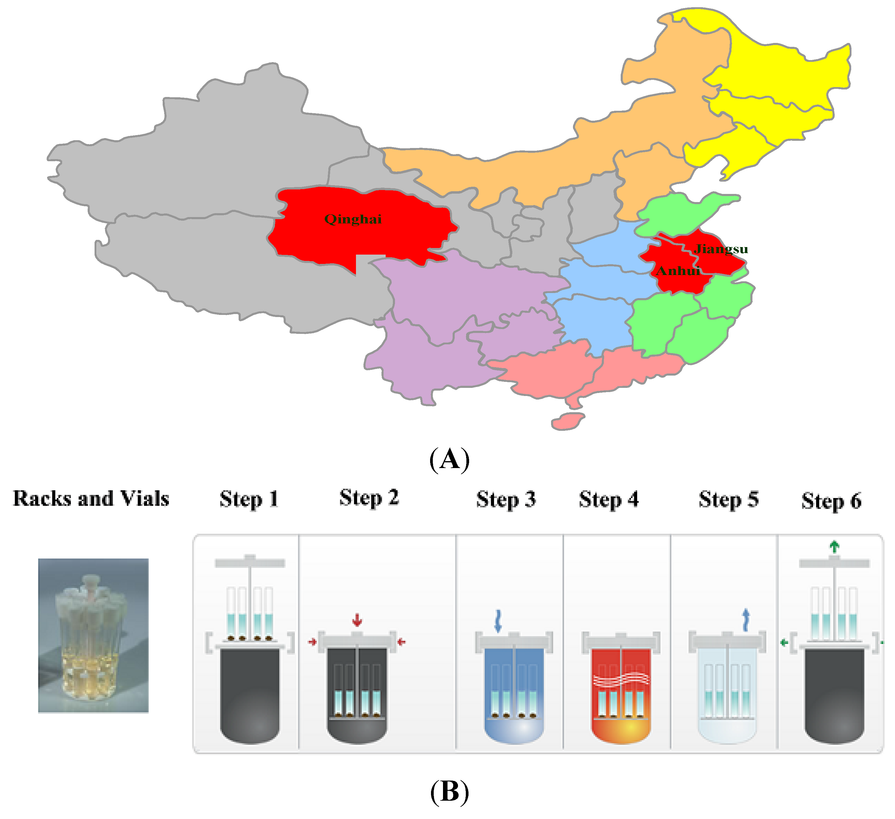
In this study, one batch of SO sample obtained from Jiangsu was used to optimize the digestion conditions by BBD (
Figure 1), and its blank and spiked samples were pretreated in parallel three times. Then the recovery was calculated as follows:
Figure 1.
Origins of the samples and the ultrawave digestion procedure. (A) The distribution of the 18 batches of SO in China; (B) The ultrawave digestion procedure.
Figure 1.
Origins of the samples and the ultrawave digestion procedure. (A) The distribution of the 18 batches of SO in China; (B) The ultrawave digestion procedure.
Finally, the optimal conditions for digestion were screened out by BBD. The ultrawave digestion procedure is shown in
Table 1. Operating conditions and parameters for the ICP-MS and ultrawave single reaction chamber microwave digestion systems are shown in
Table S1. As shown in
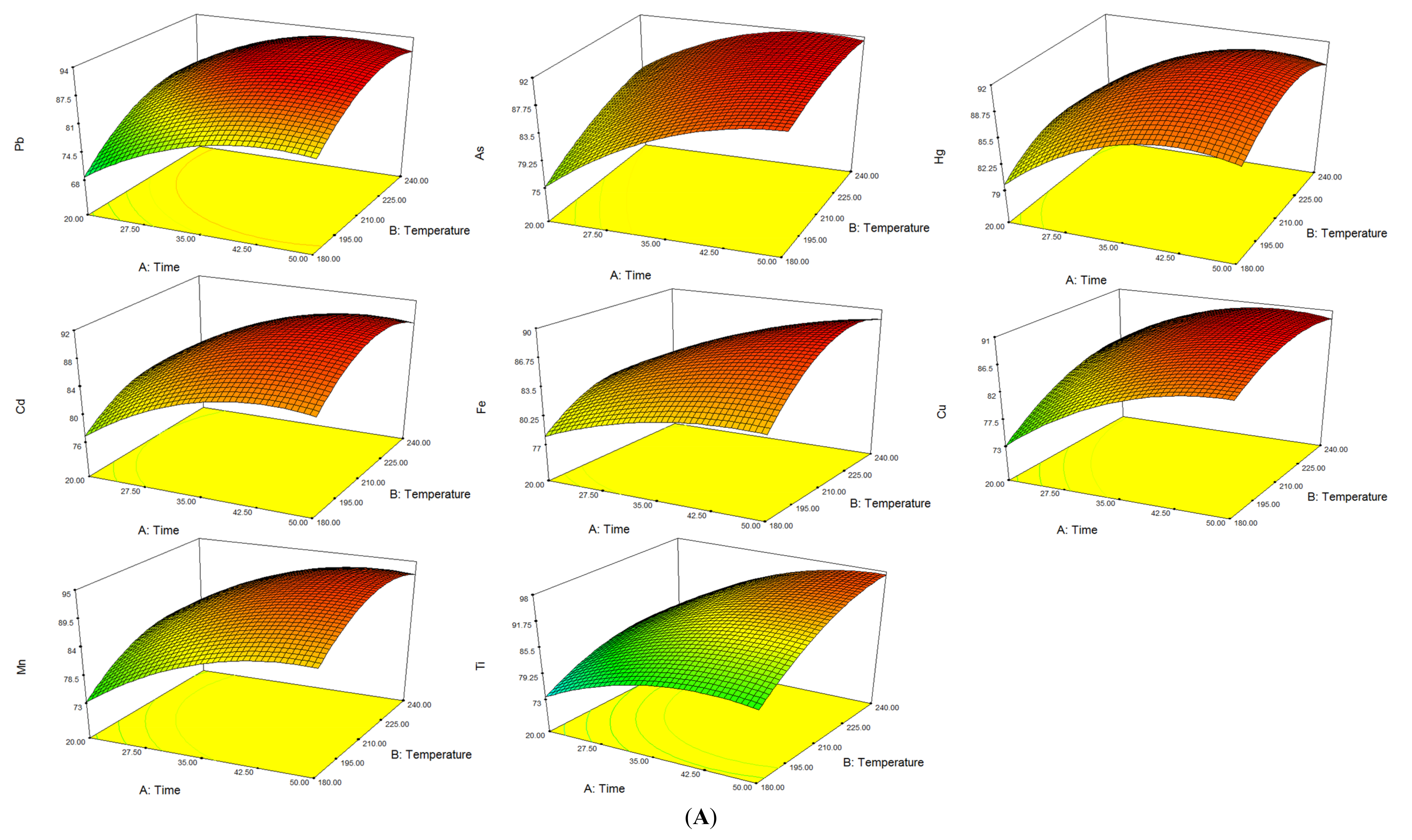
Table S2, three digestion variables including temperature (A), time (B) and pressure (C) were examined by BBD design. In this optimization, the recoveries of 14 metal elements were chosen as the response. Comprehensive test results of response surface plots (3D) showed that the recoveries of 14 elements were all higher than 80% under the experimental conditions of temperature at 210 °C, pressure at 90 bar and digestion time for 35 min.
Table 1.
Ultrawave digestion procedure.
Table 1.
Ultrawave digestion procedure.
| Steps | Status | Temperature/°C | Time/min |
|---|
| 1 | 1600 W heating | 25–120 | 5 |
| 2 | Insulation | 120 | 5 |
| 3 | 1600 W heating | 120–210 | 5 |
| 4 | Insulation | 210 | 35 |
The experimental data was analyzed by ANOVA and the results are given in
Table 2 and
Table S2. Values of “prob > F” less than 0.001 indicated that the model terms are significant. R-Squared higher than 0.99 for less than 1.0% of the total variations, indicated that the optimal results were accurate and reliable. Therefore, we could find out the optimal condition from (3D) response surface plots was a temperature at 210 °C while the pressure was kept at 90 bar for 35 min (
Figure 2). The correlation coefficient of 14 elements were all at 0.99 under ICP-MS conditions, while the standard curves were forced through the origin. Blank sample was repeatedly testing 10 times, and three times the standard deviation was the limit of detection (LOD), and 10 times the standard deviation was the limit of quantitation (LOQ). The LOD were 0.002–0.6 μg/kg, LOQ were 0.335–9.1 μg/kg, the recovery rates of 14 standards varied from 86.5%–99.2% (
Table 3), revealing the accuracy of this method.
Table 2.
ANOVA for response surface model.
Table 2.
ANOVA for response surface model.
| Response | Final Equation | Std. Dev. | Mean | C.V. % | PRESS | R-Squared |
|---|
| Pb | Pb = 85.72 + 3.82A + 4.94B + 10.24C − 0.97AB + 2.28AC + 1.05BC − 5.03A2 − 4.68B2 − 4.79C2 | 6.32 | 75.81 | 8.34 | 2913.15 | 0.9021 |
| As | As = 83.56 + 4.29A + 2.96B + 11.96C − 1.36AB + 1.69AC − 0.44BC − 3.30A2 − 1.20B2 − 5.46C2 | 5.57 | 76.76 | 7.26 | 2152.43 | 0.9035 |
| Hg | Hg = 84.15 + 2.78A + 2.02B + 13.83C + 0.15AB + 1.48AC − 1.62BC − 3.74A2 − 2.89B2 − 5.56C2 | 4.95 | 75.81 | 6.52 | 1632.57 | 0.9341 |
| Cd | Cd = 82.92 + 3.13A + 2.37B + 13.21C + 0.30AB + 1.88AC − 1.27BC − 3.40A2 − 3.58B2 − 5.07C2 | 5.88 | 74.69 | 7.87 | 2239.73 | 0.9038 |
| Fe | Fe = 81.10 + 1.80A + 1.80B + 11.51C + 1.20AB + 2.23AC + 0.53BC − 1.48A2 − 3.25B2 − 4.19C2 | 4.58 | 75.01 | 6.10 | 1054.59 | 0.9175 |
| Cu | Cu = 83.23 + 3.44A + 4.06B + 10.68C − 1.36AB + 2.51AC − 1.36BC − 3.46A2 − 2.27B2 − 4.25C2 | 4.77 | 76.42 | 6.25 | 955.60 | 0.9151 |
| Mn | Mn = 85.88 + 5.23A + 4.67B + 10.41C − 0.50AB + 1.60AC − 2.02BC − 4.09A2 − 4.20B2 − 2.82C2 | 5.40 | 78.30 | 6.90 | 1939.88 | 0.9031 |
| Ti | Ti = 86.85 + 5.07A + 3.30B + 8.45C + 1.96AB + 1.96AC + 3.11BC − 4.23A2 − 3.47B2 − 2.97C2 | 3.32 | 79.56 | 4.17 | 253.82 | 0.9498 |
| Ni | Ni = 89.17 + 7.35A + 3.41B + 9.18C + 0.89AB + 3.39AC − 1.64BC − 6.99A2 − 3.68B2 − 2.36C2 | 3.92 | 80.27 | 4.89 | 726.98 | 0.9517 |
| V | V = 87.65 + 7.26A + 2.41B + 9.21C + 0.85AB + 6.05AC − 3.25BC − 5.74A2 − 2.96B2 − 4.18C2 | 3.23 | 78.85 | 4.10 | 789.74 | 0.9671 |
| Cr | Cr = 86.95 + 5.05A + 1.37B + 8.23C + 2.34AB + 2.14AC − 0.39BC − 6.88A2 − 2.58B2 − 3.33C2 | 6.02 | 78.22 | 7.70 | 2293.24 | 0.9060 |
| Na | Na = 73.30 + 2.44A + 4.97B + 10.24C − 0.075AB + 3.30AC + 2.08BC − 10.32A2 + 0.30B2 − 4.91C2 | 5.70 | 63.11 | 9.04 | 2112.79 | 0.9205 |
| K | K = 71.15 + 0.54A + 2.90B + 9.96C − 2.14AB + 3.66AC + 2.99BC − 9.80A2 + 0.29B2 − 5.65C2 | 6.64 | 60.80 | 10.92 | 3005.07 | 0.9062 |
| Ca | Ca = 78.15 + 1.02A + 0.82B + 8.36C + 1.79AB − 2.49AC + 2.54BC − 7.43A2 − 1.53B2 − 4.41C2 | 4.92 | 69.03 | 7.12 | 1449.21 | 0. 9176 |
Table 3.
The linear regression equations, the correlation coefficient (r), method detection limits(LOD, LOQ), precision, repeatability, and recovery of 14 elements under ICP-MS conditions.
Table 3.
The linear regression equations, the correlation coefficient (r), method detection limits(LOD, LOQ), precision, repeatability, and recovery of 14 elements under ICP-MS conditions.
| Elements | Linear equation | Linearity range μg/L | r | LOD μg/kg | LOQ μg/kg | Precision (RSD, n = 6) % | Repeatability (RSD, n = 6) % | Recovery (%) |
|---|
| Intraday | Interday |
|---|
| Pb | Y = 66211X | 0–10 | 0.9998 | 0.005 | 0.353 | 1.23 | 1.56 | 2.36 | 97.8 |
| As | Y = 1487.9X | 0–5000 | 1.0000 | 0.02 | 2.56 | 2.31 | 2.43 | 2.07 | 98.6 |
| Hg | Y = 6572.3X | 0–10 | 1.0000 | 0.004 | 0.708 | 1.43 | 1.63 | 3.24 | 96.4 |
| Cd | Y = 3955.5X | 0–10 | 1.0000 | 0.002 | 0.335 | 2.03 | 2.34 | 2.78 | 98.3 |
| Fe | Y = 215.19X | 0–5000 | 0.9981 | 0.09 | 3.64 | 1.78 | 2.44 | 2.78 | 97.4 |
| Cu | Y = 14242 X | 0–10 | 0.9996 | 0.008 | 3.091 | 2.58 | 1.96 | 3.35 | 88.7 |
| Mn | Y = 7966.1X | 0–50 | 1.0000 | 0.02 | 5.18 | 2.32 | 2.55 | 2.23 | 93.8 |
| Ti | Y = 168.39X | 0–500 | 0.9993 | 0.2 | 5.8 | 1.73 | 2.05 | 2.19 | 86.5 |
| Ni | Y = 10693X | 0–50 | 0.9982 | 0.009 | 5.668 | 1.99 | 2.57 | 2.47 | 90.4 |
| V | Y = 9399.3X | 0–10 | 1.0000 | 0.003 | 2.608 | 2.27 | 2.79 | 2.94 | 96.5 |
| Cr | Y = 1441.2X | 0–50 | 1.0000 | 0.002 | 6.088 | 1.66 | 2.16 | 2.38 | 99.2 |
| Na | Y = 45249X | 0–5000 | 0.9988 | 0.2 | 9.1 | 1.07 | 2.76 | 3.76 | 89.7 |
| K | Y = 15646X | 0–5000 | 0.9979 | 0.6 | 8.1 | 2.06 | 2.37 | 2.89 | 90.2 |
| Ca | Y = 51.87X | 0–500 | 0.9975 | 0.3 | 5.1 | 1.65 | 2.39 | 3.25 | 87.9 |
2.2. Application to Multielemental Analysis in SO
In this study, fourteen elements in SO samples were successfully determined to compare each one. Under our experimental conditions, the digested solutions containing of the fourteen elements, including Pb, As, Hg, Cd, Fe, Cu, Mn, Ni, Ti, V, Cr, Na, K and Ca, were directly injected and analyzed after constant volume.
As shown in
Table 4, an obvious difference in the concentrations of all 14 elements was observed in different SO samples. The contents of elements detected in various samples were in the range from 0.0015 to 1.4 mg/kg for Pb, from 0.013 to 784 mg/kg for As, from 0.0015 to 0.025 mg/kg for Hg, from 0.239 to 1.61 mg/kg for Cu, from 196 to 817 mg/kg for Na, from 94 to 584 mg/kg for K, from 18 to 80 mg/kg for Ca, from 3.81 to 21 mg/kg for Ti, from 0.079 to 0.274 mg/kg for V, from 4.00 to 9.81 mg/kg for Cr, from 0.61 to 2.03 mg/kg for Mn, and from 71.6 to 224 mg/kg for Fe.
Among the analyzed elements, Na was the most abundant element, followed by K, Fe, Ca, Ti, Cr, Ni, Mn, Cu, V, As, Pb, Hg, and Cd. In particular, the content of elements such as Pb, As, Hg, Cd, V were very low. However, a high amount of As was found in batches 5 and 6 (784 mg/kg and 561 mg/kg), which might have been contaminated during preparation or storage. Concentrations of Na, K, Ca, and Fe were more higher than other elements in the SO, especially in batches 1, 6, 7, and 8. Unexpectedly, Cd and Ni were not detected in batches 1–4, 14, and 15, 18, respectively.
Figure 2.
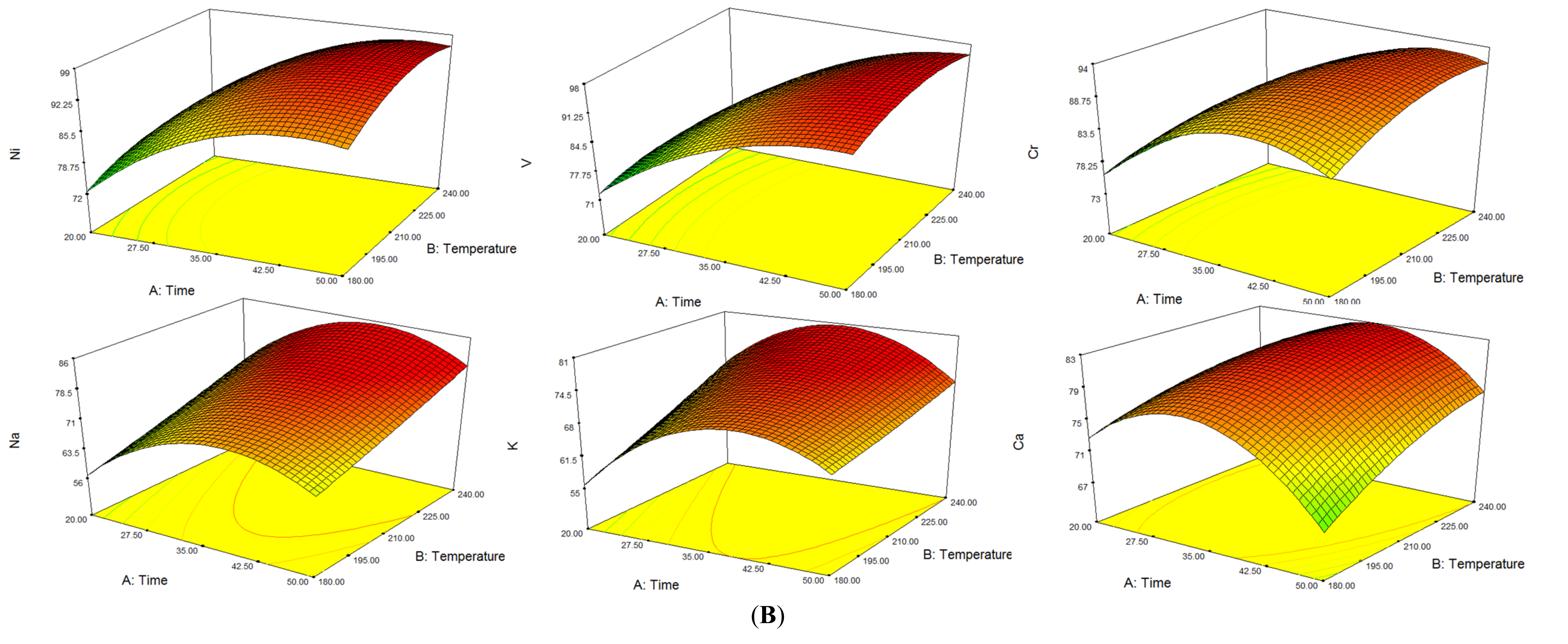
Optimization of ultrawave digestion parameters by BBD. (A) Response surface plots (3 D) of Pb, As, Hg, Cd, Fe, Cu, Mn, Ti; (B) Response surface plots (3 D) of Ni, V, Cr, Na, K, Ca.
Figure 2.
Optimization of ultrawave digestion parameters by BBD. (A) Response surface plots (3 D) of Pb, As, Hg, Cd, Fe, Cu, Mn, Ti; (B) Response surface plots (3 D) of Ni, V, Cr, Na, K, Ca.
Table 4.
Contents of 14 types elements in 18 batchs of suet oil (n = 3).
Table 4.
Contents of 14 types elements in 18 batchs of suet oil (n = 3).
| Origins | Batches | Content (mean ± SD, mg/kg) |
|---|
| Pb | As | Cd | Hg | Cu | Na | K | Ca | Ti | V | Cr | Mn | Fe | Ni |
|---|
| Anhui | 1 | 0.0015 ± 0.0008 | 0.013 ± 0.005 | nd | 0.004 ± 0.001 | 0.82 ± 0.01 | 817 ± 4 | 584 ± 5 | 80 ± 4 | 21 ± 1 | 0.274 ± 0.007 | 9.81 ± 0.03 | 2.03 ± 0.03 | 224 ± 5 | 2.45 ± 0.06 |
| 2 | 0.18 ± 0.01 | 0.093 ± 0.006 | nd | 0.0040 ± 0.0003 | 1.11 ± 0.09 | 386 ± 5 | 248 ± 6 | 29 ± 1 | 7.8 ± 0.1 | 0.14 ± 0.01 | 8.94 ± 0.04 | 1.03 ± 0.02 | 148 ± 6 | 1.02 ± 0.05 |
| 3 | 0.20 ± 0.01 | 0.035 ± 0.007 | nd | 0.0030 ± 0.0001 | 1.45 ± 0.02 | 411 ± 6 | 314 ± 8 | 34 ± 4 | 8.07 ± 0.04 | 0.15 ± 0.01 | 8.0 ± 0.1 | 1.16 ± 0.01 | 145 ± 3 | 1.02 ± 0.01 |
| 4 | 0.11 ± 0.01 | 0.026 ± 0.004 | nd | 0.0020 ± 0.0001 | 0.43 ± 0.01 | 323 ± 3 | 206 ± 6 | 24 ± 2 | 5.60 ± 0.06 | 0.113 ± 0.006 | 7.90 ± 0.05 | 0.816 ± 0.008 | 120 ± 5 | 0.94 ± 0.01 |
| 5 | 0.70 ± 0.03 | 784 ± 8 | 0.012 ± 0.001 | 0.0002 ± 0.0001 | 0.276 ± 0.004 | 360 ± 4 | 214 ± 5 | 26 ± 3 | 8.79 ± 0.07 | 0.150 ± 0.004 | 7.9 ± 0.1 | 1.02 ± 0.01 | 179 ± 7 | 0.593 ± 0.008 |
| 6 | 0.13 ± 0.01 | 561 ± 11 | 0.0010 ± 0.0003 | 0.0015 ± 0.0001 | 0.239 ± 0.008 | 632 ± 4 | 444 ± 9 | 59 ± 4 | 19.4 ± 0.1 | 0.172 ± 0.003 | 4.07 ± 0.05 | 1.88 ± 0.02 | 181 ± 4 | 3.79 ± 0.07 |
| Qinghai | 7 | 1.4 ± 0.1 | 0.34 ± 0.02 | 0.030 ± 0.006 | 0.025 ± 0.001 | 1.34 ± 0.02 | 580 ± 7 | 392 ± 7 | 50 ± 2 | 11.61 ± 0.01 | 0.194 ± 0.002 | 7.72 ± 0.03 | 1.36 ± 0.02 | 157 ± 4 | 1.42 ± 0.02 |
| 8 | 0.8 ± 0.1 | 0.26 ± 0.02 | 0.016 ± 0.002 | 0.015 ± 0.001 | 0.90 ± 0.02 | 703 ± 8 | 488 ± 7 | 59 ± 3 | 18.57 ± 0.08 | 0.162 ± 0.004 | 4.00 ± 0.06 | 1.68 ± 0.02 | 188 ± 2 | 2.38 ± 0.02 |
| 9 | 1.3 ± 0.1 | 0.31 ± 0.02 | 0.020 ± 0.003 | 0.020 ± 0.001 | 1.21 ± 0.01 | 291 ± 5 | 147 ± 5 | 26 ± 1 | 5.76 ± 0.08 | 0.084 ± 0.005 | 4.356 ± 0.002 | 0.91 ± 0.02 | 93.1 ± 0.2 | 0.59 ± 0.03 |
| 10 | 1.4 ± 0.1 | 0.30 ± 0.02 | 0.027 ± 0.003 | 0.018 ± 0.001 | 1.49 ± 0.02 | 320 ± 5 | 159 ± 5 | 29 ± 3 | 4.82 ± 0.07 | 0.224 ± 0.009 | 6.570 ± 0.002 | 0.91 ± 0.01 | 151 ± 3 | 2.52 ± 0.02 |
| 11 | 1.2 ± 0.1 | 0.273 ± 0.008 | 0.021 ± 0.001 | 0.0165 ± 0.0004 | 1.606 ± 0.006 | 426 ± 5 | 253 ± 6 | 41 ± 3 | 8.2 ± 0.1 | 0.142 ± 0.001 | 7.074 ± 0.006 | 1.04 ± 0.01 | 126 ± 2 | 0.99 ± 0.01 |
| Jiangsu | 12 | 0.9 ± 0.1 | 0.104 ± 0.009 | 0.013 ± 0.001 | 0.013 ± 0.001 | 0.844 ± 0.006 | 296 ± 8 | 170 ± 6 | 27 ± 2 | 6.17 ± 0.04 | 0.1005 ± 0.0008 | 7.12 ± 0.04 | 0.79 ± 0.01 | 90.9 ± 0.8 | 2.74 ± 0.03 |
| 13 | 0.8 ± 0.1 | 0.04 ± 0.01 | 0.003 ± 0.001 | 0.0095 ± 0.0002 | 0.589 ± 0.009 | 306 ± 6 | 170 ± 6 | 22 ± 1 | 4.95 ± 0.04 | 0.099 ± 0.008 | 7.158 ± 0.013 | 0.72 ± 0.05 | 89 ± 2 | 0.86 ± 0.04 |
| 14 | 1.2 ± 0.1 | 0.226 ± 0.006 | nd | 0.023 ± 0.002 | 0.90 ± 0.01 | 246 ± 6 | 127 ± 7 | 23 ± 1 | 4.16 ± 0.03 | 0.095 ± 0.002 | 6.08 ± 0.04 | 0.73 ± 0.05 | 83 ± 1 | 0.52 ± 0.02 |
| 15 | 0.8 ± 0.1 | 0.21 ± 0.02 | 0.0055 ± 0.0003 | 0.0065 ± 0.0002 | 0.586 ± 0.007 | 196 ± 5 | 94 ± 2 | 18 ± 2 | 4.55 ± 0.04 | 0.079 ± 0.003 | 5.15 ± 0.03 | 0.62 ± 0.06 | 79 ± 2 | nd |
| 16 | 0.7 ± 0.1 | 0.212 ± 0.008 | 0.0030 ± 0.0008 | 0.0090 ± 0.0008 | 0.53 ± 0.01 | 264 ± 5 | 122 ± 3 | 22 ± 2 | 3.81 ± 0.02 | 0.092 ± 0.002 | 5.96 ± 0.04 | 0.62 ± 0.01 | 83.8 ± 0.5 | 0.134 ± 0.002 |
| 17 | 0.70 ± 0.07 | 0.12 ± 0.01 | 0.0030 ± 0.0008 | 0.0085 ± 0.0003 | 0.756 ± 0.007 | 301 ± 6 | 141 ± 2 | 28 ± 2 | 4.10 ± 0.04 | 0.094 ± 0.004 | 5.98 ± 0.06 | 0.753 ± 0.006 | 85.8 ± 0.4 | 1.22 ± 0.01 |
| 18 | 0.91 ± 0.08 | 0.041 ± 0.006 | 0.006 ± 0.001 | 0.0095 ± 0.0004 | 0.620 ± 0.004 | 294 ± 4 | 141 ± 3 | 22 ± 2 | 4.0 ± 0.2 | 0.086 ± 0.002 | 5.92 ± 0.02 | 0.61 ± 0.01 | 71.6 ± 0.8 | nd |
2.3. PCA of the SO Samples
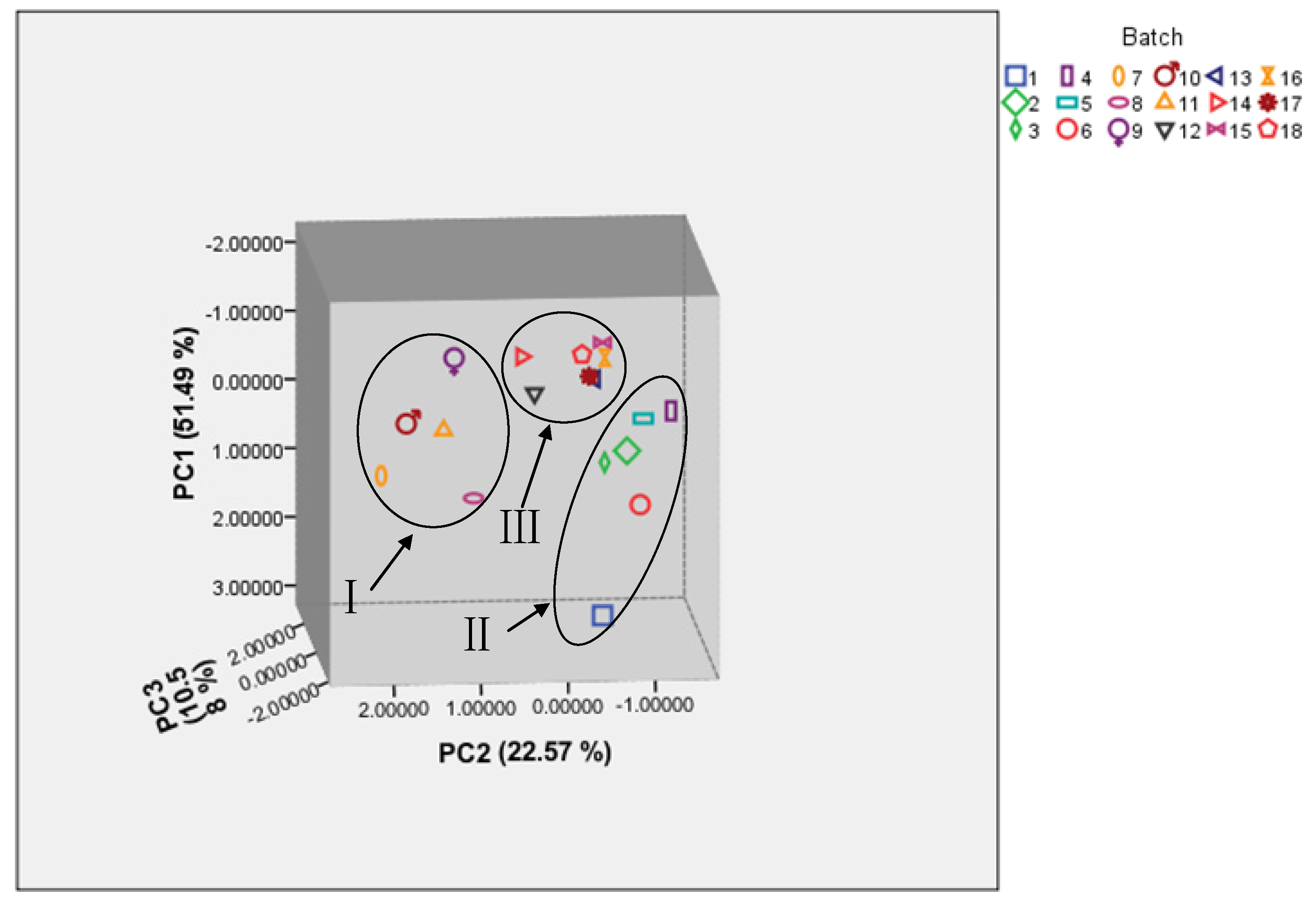
To evaluate the variation of SO, PCA was performed on the basis of the contents of 14 tested elements from SO. The first three principal components (PC1, PC2, and PC3) with >84.6% of the whole variance were extracted for analysis. Among them, PC1 accounted for 51.49% of total variance, whereas PC2 and PC3 for 22.57% and 10.58%, respectively. The remaining principal components were discarded due to their minor effects on the model. The correlation matrix of PCA analysis for 14 elements is shown in
Table S3. The total variance for PCA and the components loading matrix is shown in
Table 5 and
Table 6. According to their loadings, PC1 had good correlation with the 14 elements. The above results suggested that most of the elements might contribute to the classification of the samples.
Table 5.
The total variance explained for PCA of 14 elements in 18 batches of SO.
Table 5.
The total variance explained for PCA of 14 elements in 18 batches of SO.
| Component | Initial Eigenvalues | Extraction Sums of Squared Loadings |
|---|
| Total | % of Variance | Cumulative % | Total | % of Variance | Cumulative % |
|---|
| 1 | 7.209 | 51.491 | 51.491 | 7.209 | 51.491 | 51.491 |
| 2 | 3.160 | 22.572 | 74.062 | 3.160 | 22.572 | 74.062 |
| 3 | 1.482 | 10.586 | 84.649 | 1.482 | 10.586 | 84.649 |
| 4 | 0.951 | 6.794 | 91.443 | | | |
| 5 | 0.479 | 3.423 | 94.866 | | | |
| 6 | 0.301 | 2.153 | 97.019 | | | |
| 7 | 0.179 | 1.280 | 98.299 | | | |
| 8 | 0.134 | 0.960 | 99.259 | | | |
| 9 | 0.059 | 0.418 | 99.677 | | | |
| 10 | 0.019 | 0.133 | 99.810 | | | |
| 11 | 0.014 | 0.102 | 99.913 | | | |
| 12 | 0.008 | 0.060 | 99.973 | | | |
| 13 | 0.003 | 0.018 | 99.991 | | | |
| 14 | 0.001 | 0.009 | 100.000 | | | |
Table 6.
The component matrix of PCA analysis for 14 elements in 18 batches of SO.
Table 6.
The component matrix of PCA analysis for 14 elements in 18 batches of SO.
| Elements | Component |
|---|
| 1 | 2 | 3 |
|---|
| Pb | −0.440 | 0.825 | 0.251 |
| As | 0.294 | −0.400 | 0.563 |
| Cd | 0.032 | 0.869 | 0.205 |
| Hg | −0.232 | 0.902 | 0.108 |
| Cu | 0.018 | 0.776 | −0.469 |
| Na | 0.966 | 0.112 | 0.001 |
| K | 0.970 | 0.057 | −0.042 |
| Ca | 0.955 | 0.152 | −0.005 |
| Ti | 0.965 | −0.012 | 0.166 |
| V | 0.851 | 0.253 | −0.220 |
| Cr | 0.226 | −0.159 | −0.825 |
| Mn | 0.982 | 0.055 | 0.089 |
| Fe | 0.939 | 0.023 | −0.039 |
| Ni | 0.732 | 0.132 | 0.244 |
In order to further distinguish the diversity of SO samples from different origins, the scatter plot of the study was plotted. We observed that eighteen sample dots were successfully classified into groups I, group II, and group III corresponding to Qinghai, Anhui and Jiangsu (
Figure 3). Interestingly, dots in groups II and III were relatively nearer to each other, indicating a closer relationship among six batches from Anhui and seven batches from Jiangsu. However, dots in group I were relatively scattered, suggesting the diversification of the five Qinghai batches. This could be explained by several reasons: firstly, the land area of Qinghai Province is 722,300 square kilometers, larger than Anhui (139,600) and Jiangsu (106,700 square kilometers), which creates advantageous conditions for the diversity of the samples. Secondly, the climate and environment in Qinghai, Anhui and Jiangsu have great differences, which affects the differences in elemental metabolism in
Ovis aries Linnaeus or
Capra hircus Linnaeus. Thirdly, Anhui Province and Jiangsu Province are neighboring to each other in geographic location, which is the main reason for the closer results of the samples from the two origins.
Figure 3.
The 3 D scatter plots obtained from PCA of 18 batches SO samples.
Figure 3.
The 3 D scatter plots obtained from PCA of 18 batches SO samples.


