4.1. Optimization of Geometrical Parameters
Geometry optimization is a name for the procedure that attempts to find the configuration of minimum energy of the molecule. The procedure calculates the wave function and the energy at a starting geometry and then proceeds to search a new geometry of a lower energy.
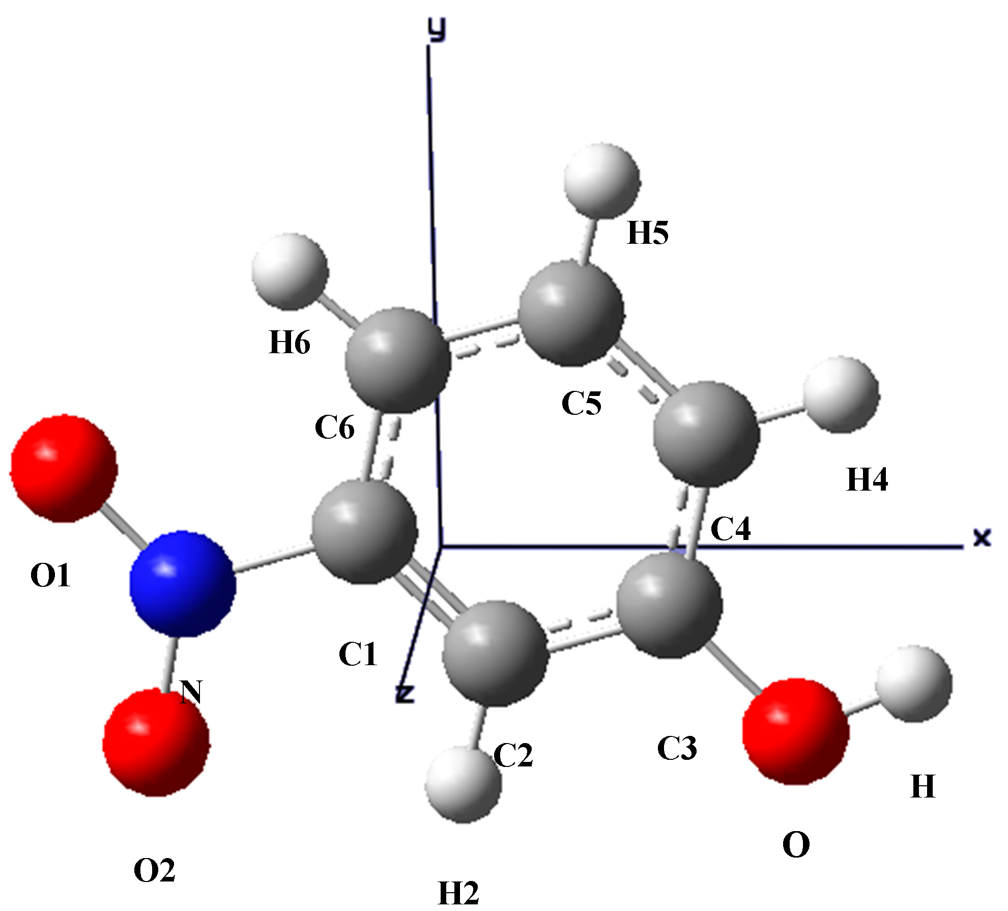
Figure 2.
The optimized structure of m-NPH based on DFT B3LYP/6-1G* basis set.
Figure 2.
The optimized structure of m-NPH based on DFT B3LYP/6-1G* basis set.
The optimized structure of the title compound is shown in
Figure 2. The calculated structure parameters (bond lengths, bond angles and torsion angles) were listed in
Table 2,
Table 3 and
Table 4 where it can be seen that all the calculated parameters are in line with the X-ray results. In summary, the optimized bond lengths and bond angles obtained using the DFT method are in good agreement with the corresponding X-ray structural parameters. The calculated geometric parameters represent a good approximation and can provide a starting point to calculate other parameters, such as vibrational wavenumbers.
Table 2.
Selected bond distances (Å) by X-ray and theoretical calculations (B3LYP/6-31G*).
Table 2.
Selected bond distances (Å) by X-ray and theoretical calculations (B3LYP/6-31G*).
| Atom 1 | Atom 2 | Distance (Å) |
|---|
| X-ray | B3LYP/6-31G* |
|---|
| C1 | C6 | 1.410 | 1.433 |
| C1 | C2 | 1.396 | 1.384 |
| C2 | C3 | 1.402 | 1.396 |
| C3 | C4 | 1.411 | 1.392 |
| C4 | C5 | 1.396 | 1.391 |
| C6 | C5 | 1.400 | 1.412 |
| O | C3 | 1.365 | 1.380 |
| C1 | N | 1.474 | 1.468 |
| O1 | N | 1.244 | 1.281 |
| O2 | N | 1.243 | 1.283 |
| O | H | 1.030 | 0.992 |
| H6 | C6 | 1.089 | 1.084 |
| H2 | C2 | 1.085 | 1.078 |
| H4 | C4 | 1.078 | 1.069 |
| H5 | C5 | 1.085 | 1.082 |
Table 3.
Selected bond angles (°) by X-ray and theoretical calculations (B3LYP/6-31G*).
Table 3.
Selected bond angles (°) by X-ray and theoretical calculations (B3LYP/6-31G*).
| Atom 1 | Atom 2 | Atom 3 | Angle (°) |
|---|
| X-ray | B3LYP/6-31G* |
|---|
| C6 | C1 | N | 118.90 | 118.46 |
| C6 | C1 | C2 | 124.11 | 122.55 |
| N | C1 | C2 | 116.99 | 117.37 |
| H2 | C2 | C3 | 122.50 | 119.45 |
| H2 | C2 | C1 | 120.51 | 120.82 |
| C3 | C2 | C1 | 118.99 | 119.10 |
| C4 | C3 | O | 123.31 | 122.72 |
| H4 | C4 | C3 | 120.31 | 119.88 |
| H4 | C4 | C5 | 118.98 | 118.94 |
| C3 | C4 | C5 | 120.71 | 118.06 |
| H5 | C5 | C6 | 119.20 | 119.87 |
| H5 | C5 | C4 | 120.66 | 119.74 |
| C6 | C5 | C4 | 120.14 | 119.28 |
| H6 | C6 | C5 | 119.39 | 120.13 |
| H6 | C6 | C1 | 123.00 | 120.91 |
| C5 | C6 | C1 | 117.60 | 119.28 |
| H | O | C3 | 109.00 | 110.55 |
| O2 | N | O1 | 123.70 | 122.07 |
| O2 | N | C1 | 119.09 | 117.04 |
| O1 | N | C1 | 117.20 | 117.03 |
Table 4.
Torsion angles (°) by X-ray and theoretical calculations (B3LYP/6-31G*).
Table 4.
Torsion angles (°) by X-ray and theoretical calculations (B3LYP/6-31G*).
| Atom1 | Atom 2 | Atom 3 | Atom 4 | Angle (°) |
|---|
| X-ray | B3LYP/6-31G* |
|---|
| C4 | C3 | C2 | C1 | −1.07 | 0.003 |
| C5 | C6 | C1 | C2 | 0.92 | −0.015 |
| C4 | C3 | C2 | C1 | 0.08 | 0.011 |
| H2 | C2 | C3 | C4 | 178.76 | 179.99 |
| H6 | C6 | C1 | C2 | −179.28 | −180.00 |
| H5 | C5 | C6 | C1 | 178.63 | 179.98 |
| H4 | C4 | C3 | C2 | −179.68 | −179.99 |
| O | C3 | C4 | C5 | −179.68 | −179.97 |
| H | O | C3 | C4 | −6.70 | −179.98 |
| N | C1 | C2 | C3 | −179.84 | 0.011 |
| O1 | N | C1 | C2 | 179.21 | 179.84 |
| O2 | N | C1 | C2 | 0.39 | 0.020 |
4.2. Electron Density Maps
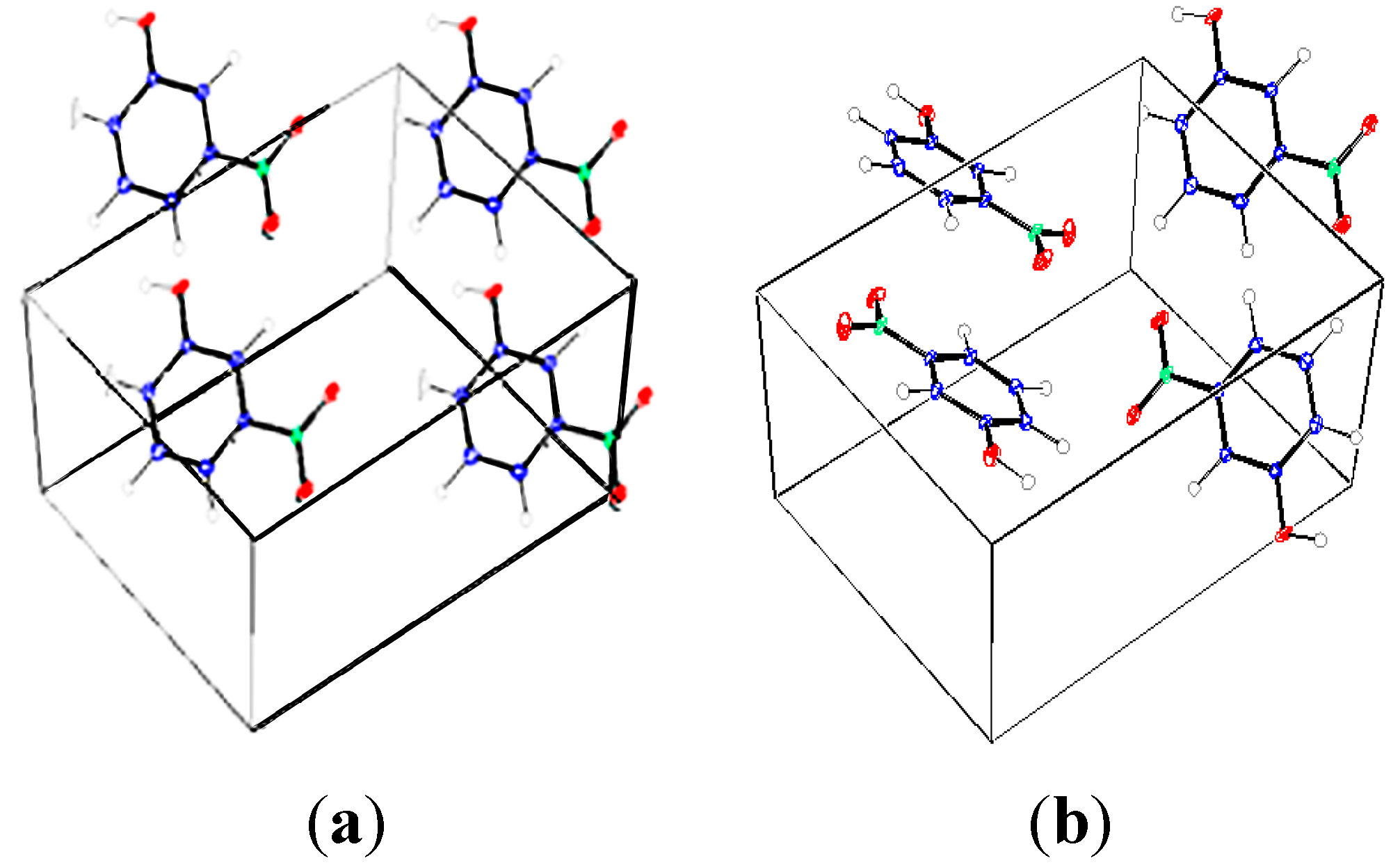
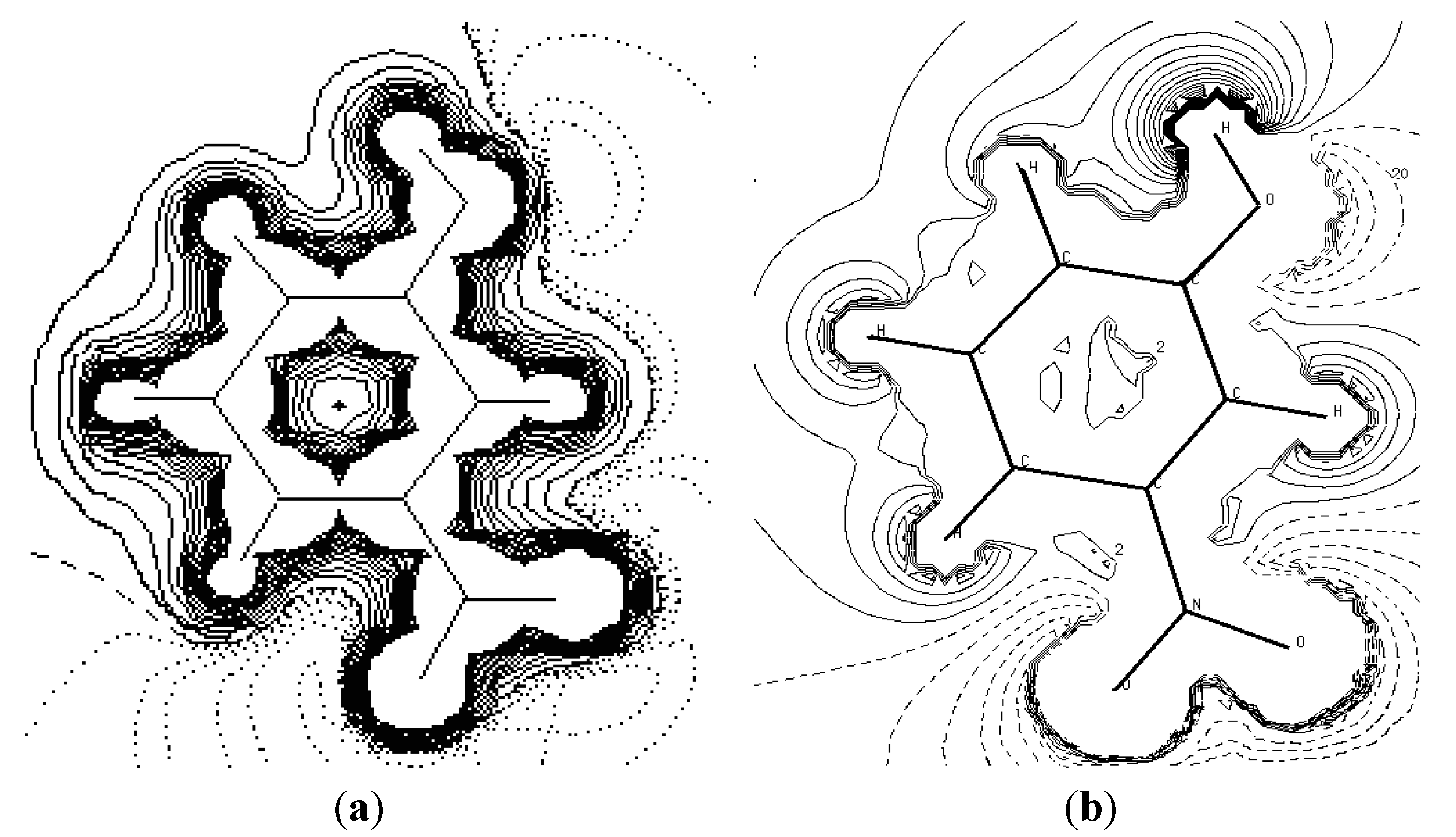
Figure 3 provides a comparison of the experimental static charge density of the molecule, obtained by convolution of the thermal motion from the charge density on the different atoms in the mean molecular plane, with the theoretical charge density, determined from a wave function for a pseudo atoms from an
ab initio calculation performed with a Gaussian basis setusing the Density Functional Theory at B3LYP level of theory at 6-31G*. As it can be seen, the two maps show reasonable agreement. These maps confirm the high quality of the data sets and the efficiency of the formalism of data processing as proposed by Blessing [
18].
Figure 3.
Comparison of the static and theoretical density maps of m-NPH. (a) Static density map. (b) Theoretical electron density map.
Figure 3.
Comparison of the static and theoretical density maps of m-NPH. (a) Static density map. (b) Theoretical electron density map.
4.3. Net Atomic Charges
Thevalence and mulitipolarpopulationceofficients were used to estimate the partial charges on the different atoms and the molecular dipole moment following the procedure described by Hansen and Coppens [
8]. The experimantal net atomic charges have been previously published in an article about the high resolution X-ray diffraction and crystallographic study of m-NPH [
5]. These values arecompared to the natural population analysis (NPA) charges derived from the
ab initio calculations using B3LYP with the 6-31G* basis set (see
Table 5,
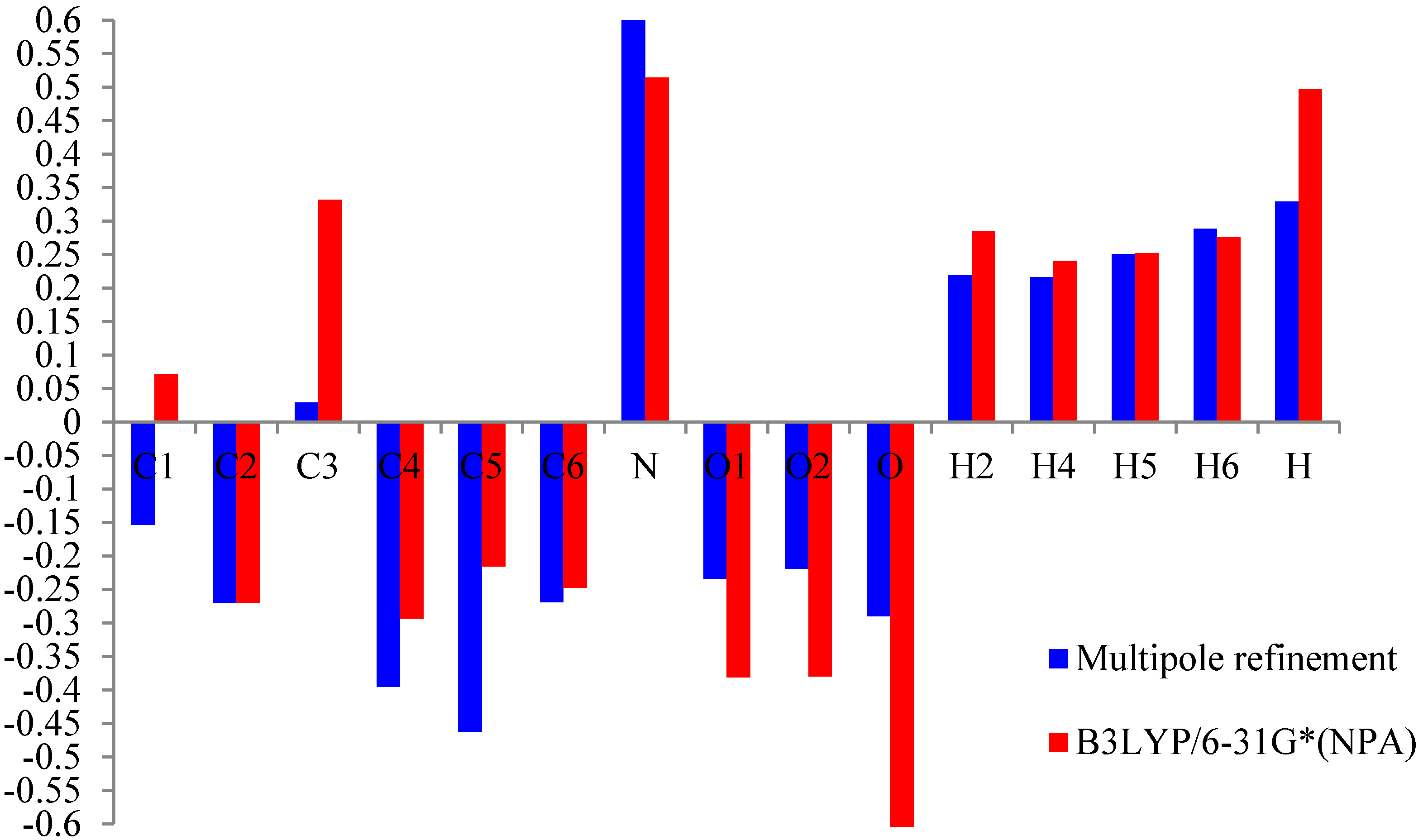
Figure 4). All the methods are in agreement for the evaluation of the positive sign of the net charges on the H and N atoms and the negative net charges on the O atoms.
Table 5.
Atomiccharge of m-nitrophenol.
Table 5.
Atomiccharge of m-nitrophenol.
| Atom | Multipolar Refinement | B3LYP/6-31G* |
|---|
| C1 | −0.1536 | 0.07099 |
| C2 | −0.2703 | −0.26992 |
| C3 | 0.0288 | 0.33201 |
| C4 | −0.3958 | −0.29354 |
| C5 | −0.4621 | −0.21591 |
| C6 | −0.2689 | −0.24740 |
| N | 0.6466 | 0.51462 |
| O1 | −0.2337 | −0.38131 |
| O2 | −0.2189 | −0.38013 |
| O | −0.2901 | −0.68228 |
| H2 | 0.2187 | 0.28515 |
| H4 | 0.2165 | 0.24054 |
| H5 | 0.2508 | 0.25207 |
| H6 | 0.2885 | 0.27564 |
| H | 0.3289 | 0.49644 |
Figure 4.
Histogram of the value of the net atomic charge in both methods multipolar refinement and B3LYP of m-nitrophenol.
Figure 4.
Histogram of the value of the net atomic charge in both methods multipolar refinement and B3LYP of m-nitrophenol.
4.4. Molecular Moments
From the knowledge of the density function one can derive some important physical properties of the molecules such as the surrounding electrostatic field gradient, and the different electrostatic moments of the charge distribution [
14]. A property associated to the average value of a quantum observable 〈
O〉 is linked to the density function as given by the general equation (3),
V is the molecular volume:
If
rather than
is being considered the electrostatic moment due to the deformation density in the molecule and can be estimated. The experimental molecular dipole moment of m-NPH has been determined in the previous paper cited above using the multipolar model [
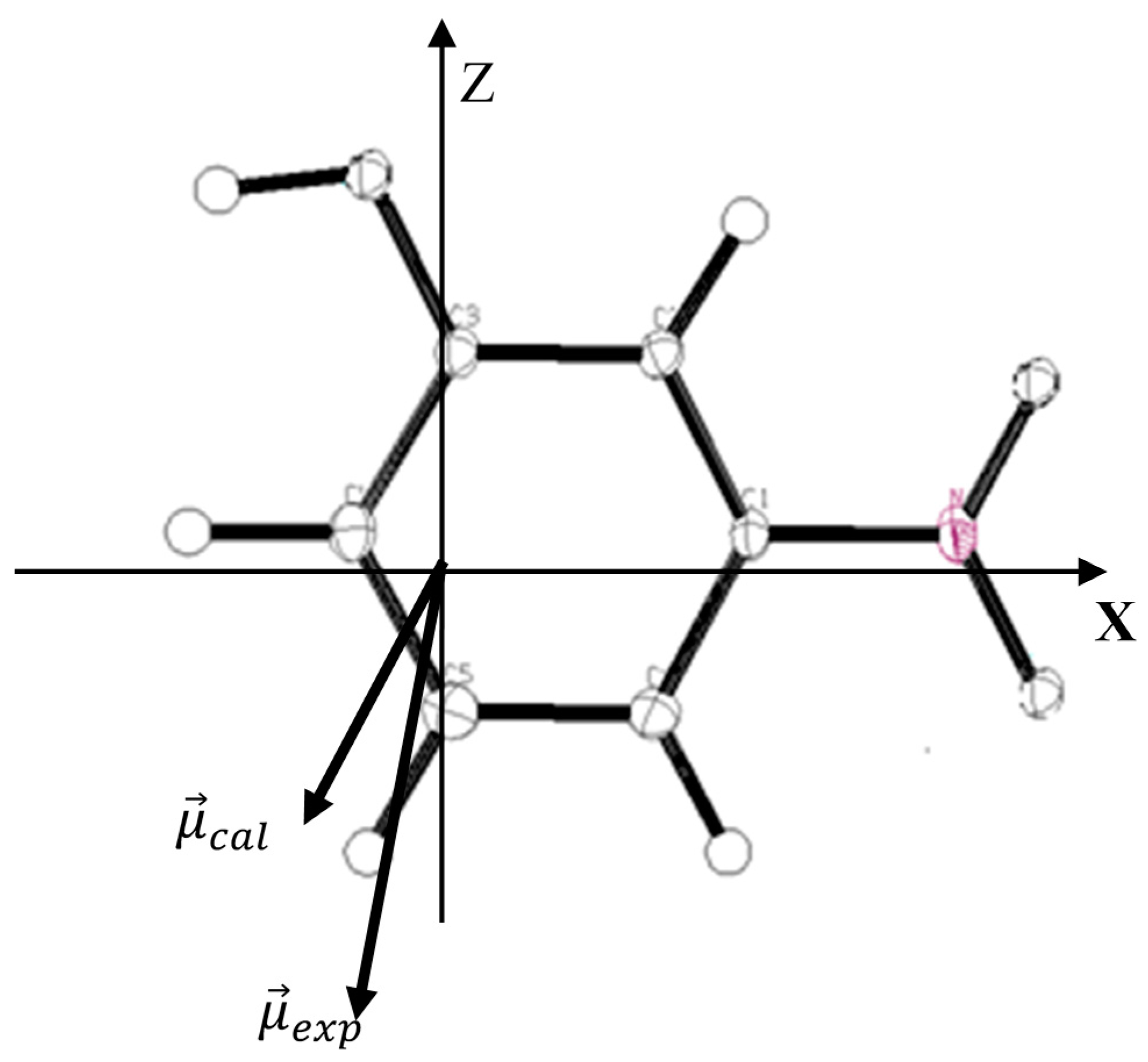
5]. Such studies have clearly evidenced the electron donor character of the C-H groups in conjunction with the electron acceptor character of the nitro and hydroxyl groups. In general, the experimental method provides a magnitude of about 5.80 Debye for the dipole moment. A theoretical calculation has been performed usingB3LYP at 6-31G* basis set in order to carried out the components of the molecular dipole moment. The obtained results are summarized in
Table 6 in which the experimental values are given for comparison. The orientation of the different vectors of dipole moment in the molecular axial system is shown in
Figure 5.
Figure 5.
Orientation of the molecular dipole moment of m-NPH: : molecular dipole moment from the experimental study; : molecular dipole moment from the theoretical DFT calculations.
Figure 5.
Orientation of the molecular dipole moment of m-NPH: : molecular dipole moment from the experimental study; : molecular dipole moment from the theoretical DFT calculations.
Table 6.
Components of the molecular dipolar moment from DFT calculations (B3LYP at 6-31G* basis set) and X-ray experiment. The origin coincides with the center of mass of the molecule, and the Cartesian system referred to the inertial axis of the molecule.
Table 6.
Components of the molecular dipolar moment from DFT calculations (B3LYP at 6-31G* basis set) and X-ray experiment. The origin coincides with the center of mass of the molecule, and the Cartesian system referred to the inertial axis of the molecule.
| Methods | Models | μX | μY | μZ | μ Debye |
|---|
| X-ray Experiment | Multipolar refinement | −0.3209 | −0.3200 | −6.3358 | 5.8000 |
| Ab initio | DFT(B3LYP/6-31G*) | −2.1194 | −0.0010 | −5.4234 | 5.8228 |
The components of the electrostatic quadrupole moment are obtained by substituting in Equation (3) the operator
Ô(r) by
. If in that equation the density function
is replaced by the multipolar expansion up to order
l = 1, then the components of the quadrupole moment are given by:
where
diα and
qi represent respectively the component of the dipole moment and the net charge of atom i at
ri.
are the atomic quadrupoles neglected here.
In the case of the direct integration method the development of Equation (3) leads to:
with:
The summation over
is performed over all structure factors and the indice
ti designates the integrable subunits. Evaluation of all molecular moments requires summations of the density and moments of each subunit which are being performed according to a space partitioning scheme. The quadrupolar moment values are reported in the
Table 7 with the analogous components obtained from the point charge model using the net atomic charges derived by NPA method calculations. The most remarkable features when comparing experimental values with those derived from the free molecule stand-out in the
QXX,
QZZ and
QXX components. The experimental second moment component relative to a chosen molecular origin, (
QXX = −55.53,
QZZ = −63.88) shows a weaker charge expansion than in the free molecule (
QXX = −53.63,
QZZ = −51.53) while the positive
QZZ’s indicate a similar contraction in the
direction (orientations in the molecular frame given in
Figure 5) for both the free molecule and the molecule in the crystal state. On the other hand the same electronic delocalization in the
direction is being observed in the molecular plane for molecules in both states.
Table 7.
Components of the molecular quadrupole moment of the charge distribution (e.Ų) from theoretical calculations and experimental electron density study.
Table 7.
Components of the molecular quadrupole moment of the charge distribution (e.Ų) from theoretical calculations and experimental electron density study.
| Quadrupole Moments | X-ray Experiment | Ab Initio DFT(6-31G) |
|---|
| QXX | −55.532 | −53.632 |
| QYY | −53.129 | −53.777 |
| QZZ | −63.886 | −51.536 |
| QXY | −1.825 | 0.964 |
| QXZ | 3.878 | 0.002 |
| QYZ | −1.755 | −0.001 |
4.6. Electrostatic Potential
In order to grasp the molecular interactions, the molecular electrostatic potential (MEP) is used. The molecular electrostatic potential is the potential that a unit positive charge would experience at any point surrounding the molecule due to the electron density distribution in the molecule. The electrostatic potential is considered predictive of chemical reactivity because regions of negative potential are expected to be sites of protonation and nucleophilic attack, while regions of positive potential may indicate electrophilic sites.The distribution of the electrostatic potential for the molecule in the crystal was calculated from Equation (7):
where
represents both the nuclear and the electronic charge. The integration is over the molecular volume, and r′ represents the atomic position relative to same origin. The integration includes the atoms of only one molecule and therefore does not include directly the effects of charge distribution of the molecules.
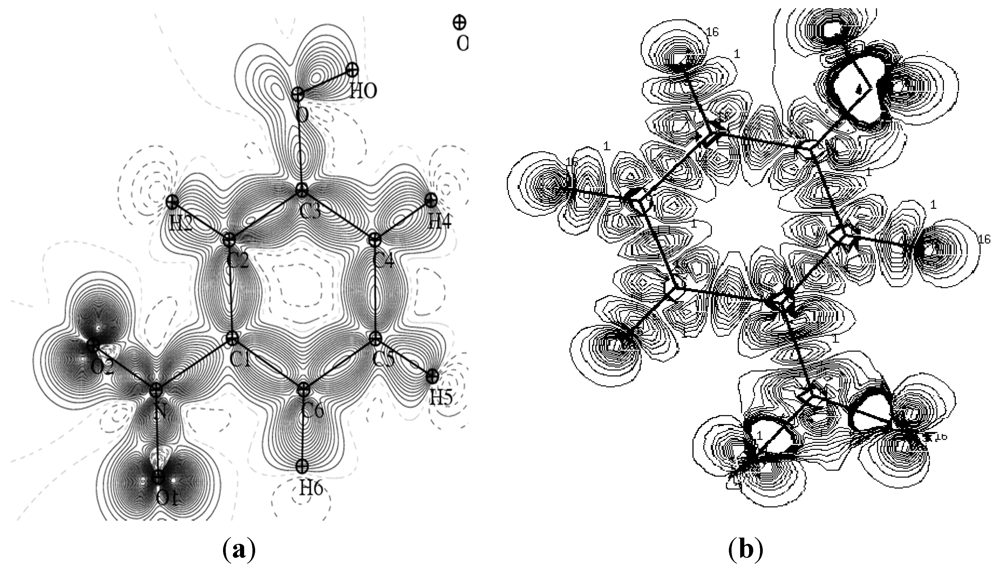
Figure 6 shows the experiment and theoretical maps of the electrostatic potential distribution in the plane of the base ring. We are used the Density Functional Theory at B3LYP level of theory at 6-31G* to describe the theoretical electrostatic potential map.
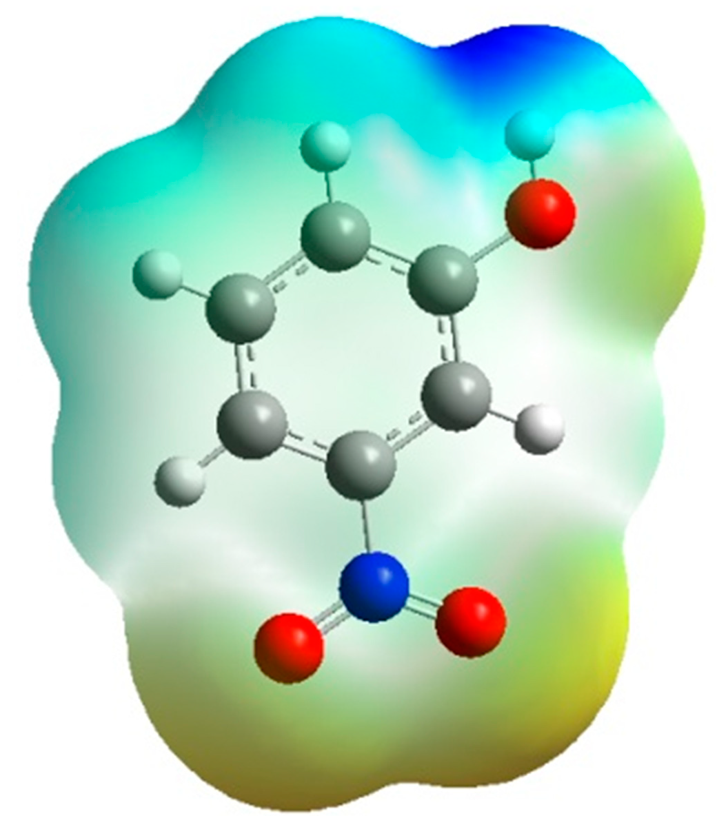
Figure 7 is the same representation in 3D dimensions of the theoretical electrostatic potential map. The extension of the positive electrostatic potential around the C-H group and the regions of negative electrostatic potential around the nitro and hydroxyl group gives same conclusion about the nature of the intramolecular charge transfer as found by the orientation of the molecular dipole moment.
Figure 6.
The electrostatic potential maps around the molecule. The section is in the plane of the ring atoms. (a) Experimental (contours are at 0.05 eǺ−1). (b) Theoreticalusing the Density Functional Theory at B3LYP level of theory at 6-31G* (contours are at 0.025 eǺ−1). Zero and negative contours are dashed lines (1 eǺ−1 = 332.1 kcal·mol−1).
Figure 7.
3D-representation of the electrostatic potential around the molecule using the Density Functional Theory at B3LYP level of theory at 6-31G*
Figure 7.
3D-representation of the electrostatic potential around the molecule using the Density Functional Theory at B3LYP level of theory at 6-31G*
The potential of the m-nitrophenol molecule has been calculated from the experimental electron density distribution by the multipolar method using the X-ray diffraction data. The comparison of the experimental potential in a crystal and the theoretical potential for an isolated molecule is an excellent test for high quality descriptive model for the electron charge density distribution from X-ray diffraction experiment.


