
Statistical Ring Opening Metathesis Copolymerization of Norbornene and Cyclopentene by Grubbs’ 1st-Generation Catalyst


 and
and 
Abstract
:
1. Introduction
2. Results and Discussion
2.1. Statistical Copolymers of NBE with CP in the Absence of Triphenylphosphine

| Sample | Mw × 10−3 Daltons | Mw/Mn c | % mol NBE d | % mol CP d |
|---|---|---|---|---|
| 20/80 | 637.5 | 1.6 | 49 | 51 |
| 40/60 | 615.8 | 1.8 | 57 | 43 |
| 50/50 | 101.1 | 1.7 | 63 | 37 |
| 60/40 | 161.5 | 1.9 | 67 | 33 |
| 80/20 | 127.1 | 1.8 | 72 | 28 |
| 20/80P | 58.4 | 1.5 | 50 | 50 |
| 40/60P | 65.7 | 1.7 | 62 | 38 |
| 50/50P | 78.2 | 1.5 | 64 | 36 |
| 60/40P | 101.4 | 1.2 | 69 | 31 |
| 80/20P | 134.3 | 1.2 | 74 | 26 |
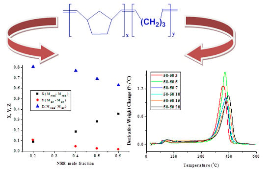
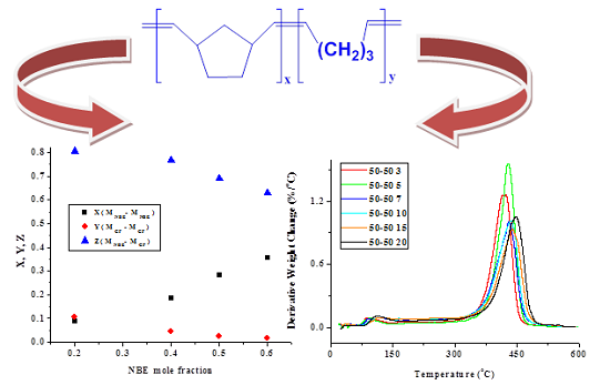
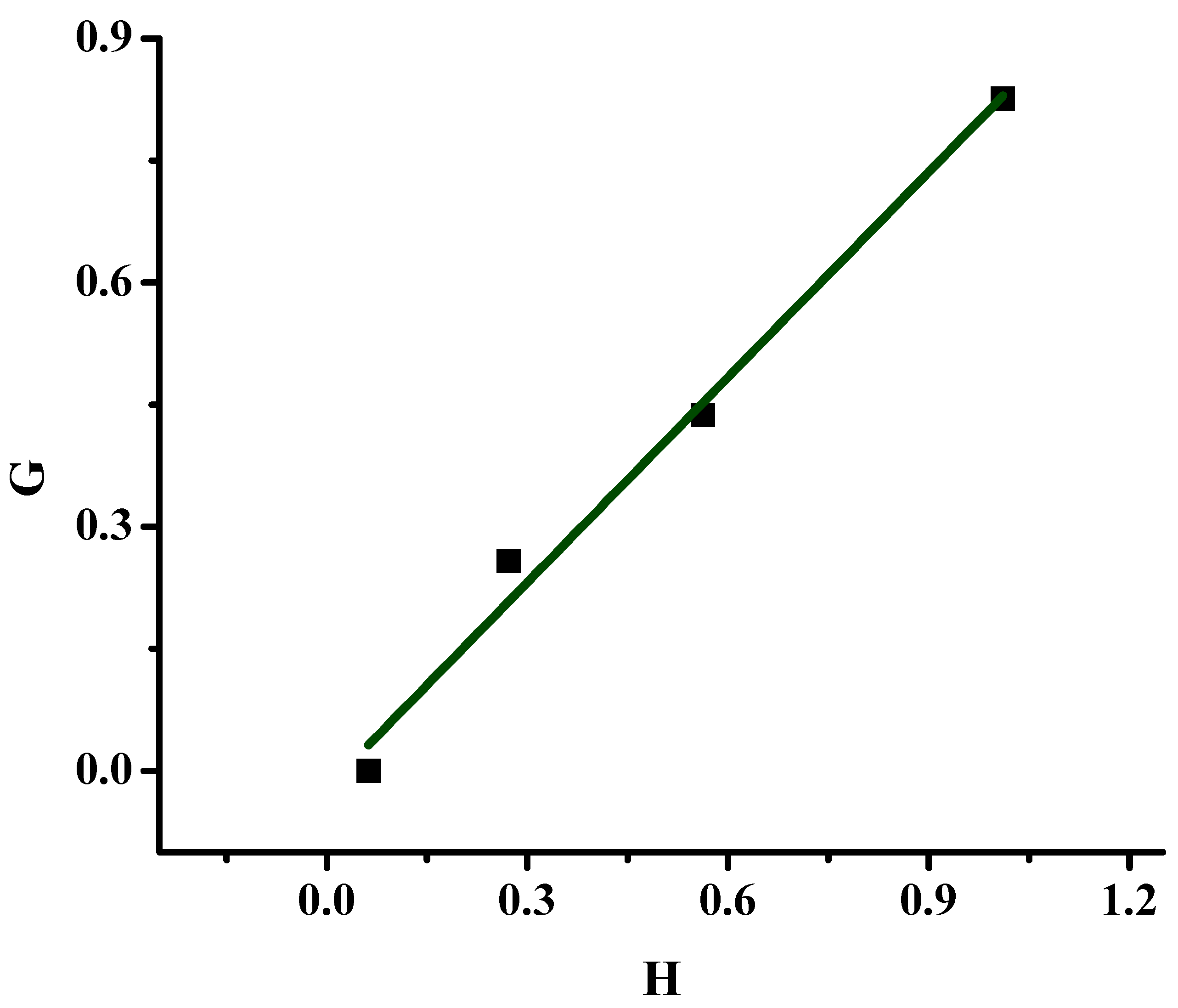
2.1.1. Monomer Reactivity Ratios and Statistical Analysis of the Copolymers
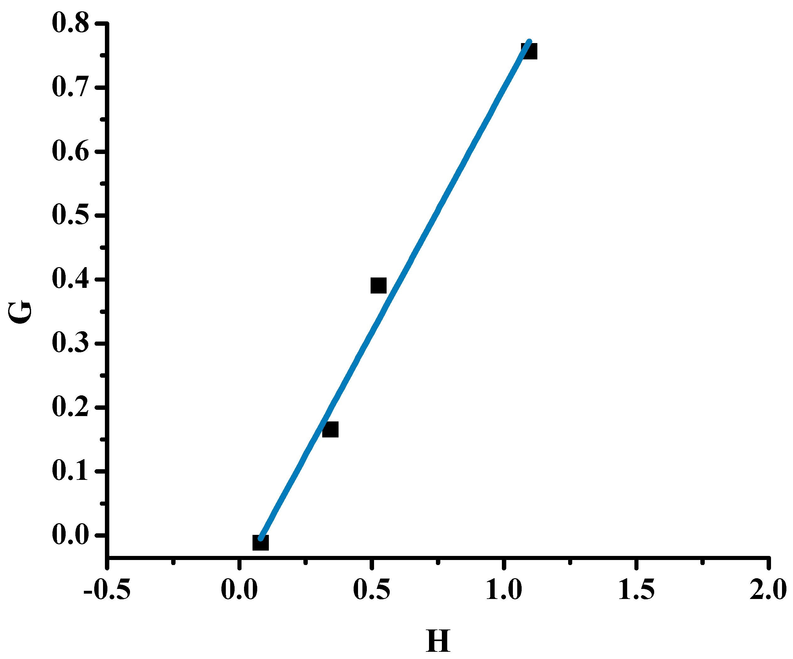
| Sample | X | Y | H | G | η | ξ |
|---|---|---|---|---|---|---|
| 20/80 | 0.277 | 0.960 | 0.080 | −0.011 | −0.030 | 0.212 |
| 40/60 | 0.675 | 1.325 | 0.344 | 0.166 | 0.259 | 0.538 |
| 50/50 | 0.946 | 1.703 | 0.525 | 0.390 | 0.475 | 0.640 |
| 60/40 | 1.491 | 2.030 | 1.095 | 0.757 | 0.544 | 0.788 |
| α = 0.295 | ||||||
| 20/80P | 0.250 | 1.000 | 0.062 | 0 | 0 | 0.199 |
| 40/60P | 0.667 | 1.631 | 0.272 | 0.258 | 0.493 | 0.520 |
| 50/50P | 1.000 | 1.778 | 0.562 | 0.437 | 0.537 | 0.691 |
| 60/40P | 1.500 | 2.226 | 1.011 | 0.826 | 0.654 | 0.801 |
| α = 0.251 |

| Method | rNBE | rCP | rNBE | rCP |
|---|---|---|---|---|
| in the Absence of PPh3 | in the Presence of PPh3 | |||
| F-R | 0.76 ± 0.06 | 0.06 ± 0.003 | 0.84 ± 0.06 | 0.02 ± 0.002 |
| i F-R | 0.78 ± 0.07 | 0.07 ± 0.004 | 0.96 ± 0.12 | 0.06 ± 0.004 |
| KT | 0.82 ± 0.10 | 0.07 ± 0.005 | 0.87 ± 0.07 | 0.02 ± 0.004 |
| COPOINT | 0.77 ± 0.14 | 0.02 ± 0.001 | 0.96 ± 0.23 | 0.03 ± 0.001 |
| Other catalytic systems a | ||||
| IrCl3/1,5-COD | 5.6 | 0.07 | ||
| WCl6/EtAlCl2 | 13 | 0.32 | ||
| WCl6/Ph4Sn | 2.6 | 0.55 | ||
| WCl6/Bu4Sn | 12 | 0.27 | ||
| WCl6/Ph4Sn/EAc | 2.2 | 0.62 | ||
| Sample | X | Y | Z | μNBE | µCP |
|---|---|---|---|---|---|
| 20/80 | 0.089 | 0.109 | 0.801 | 1.79 | 1.07 |
| 40/60 | 0.186 | 0.046 | 0.769 | 2.09 | 1.05 |
| 50/50 | 0.284 | 0.024 | 0.692 | 2.40 | 1.04 |
| 60/40 | 0.356 | 0.016 | 0.628 | 2.66 | 1.03 |
| 20/80P | 0.058 | 0.058 | 0.883 | 1.87 | 1.02 |
| 40/60P | 0.249 | 0.009 | 0.741 | 2.42 | 1.01 |
| 50/50P | 0.287 | 0.007 | 0.705 | 2.55 | 1.01 |
| 60/40P | 0.384 | 0.004 | 0.611 | 2.94 | 1.01 |
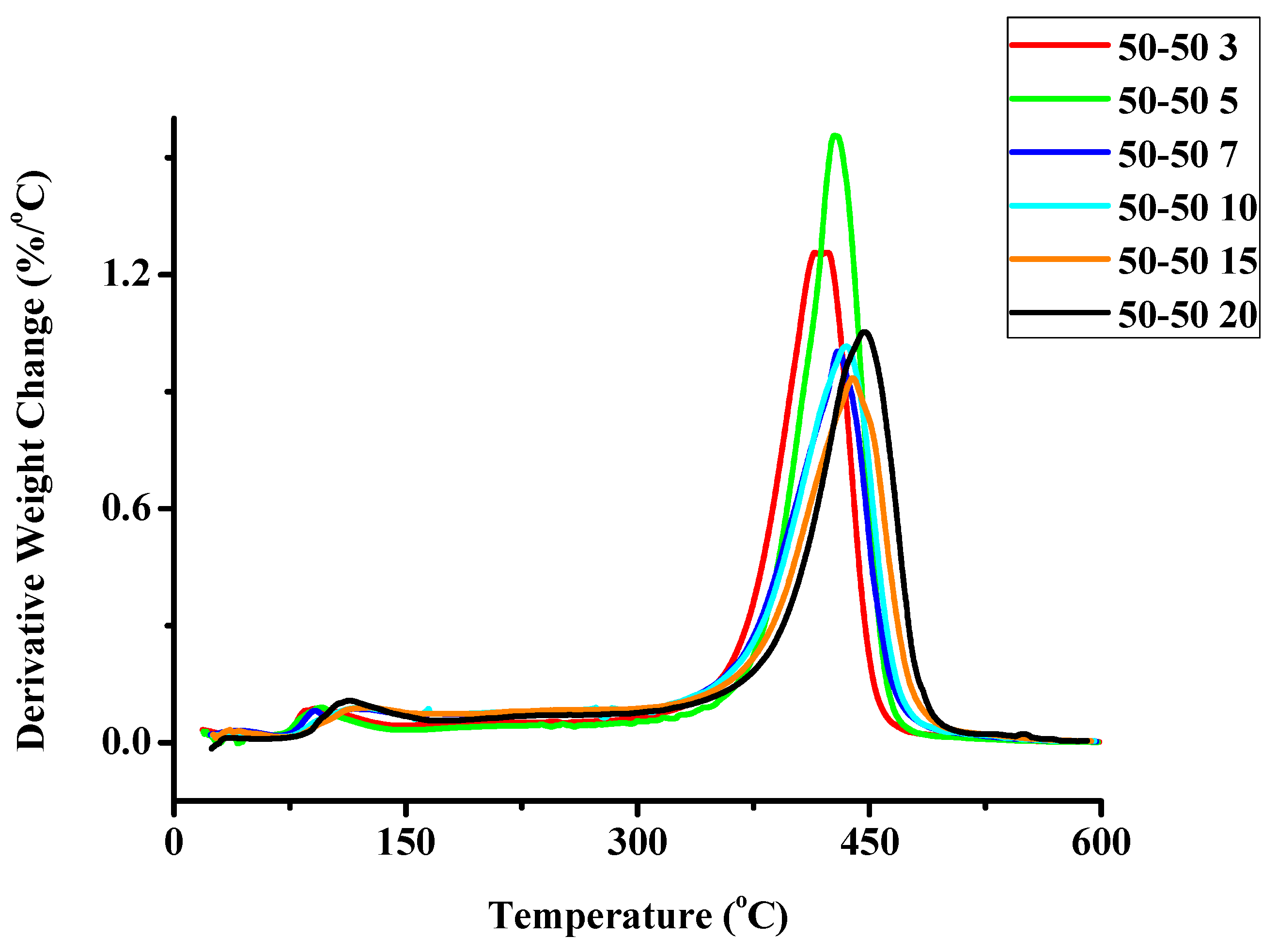
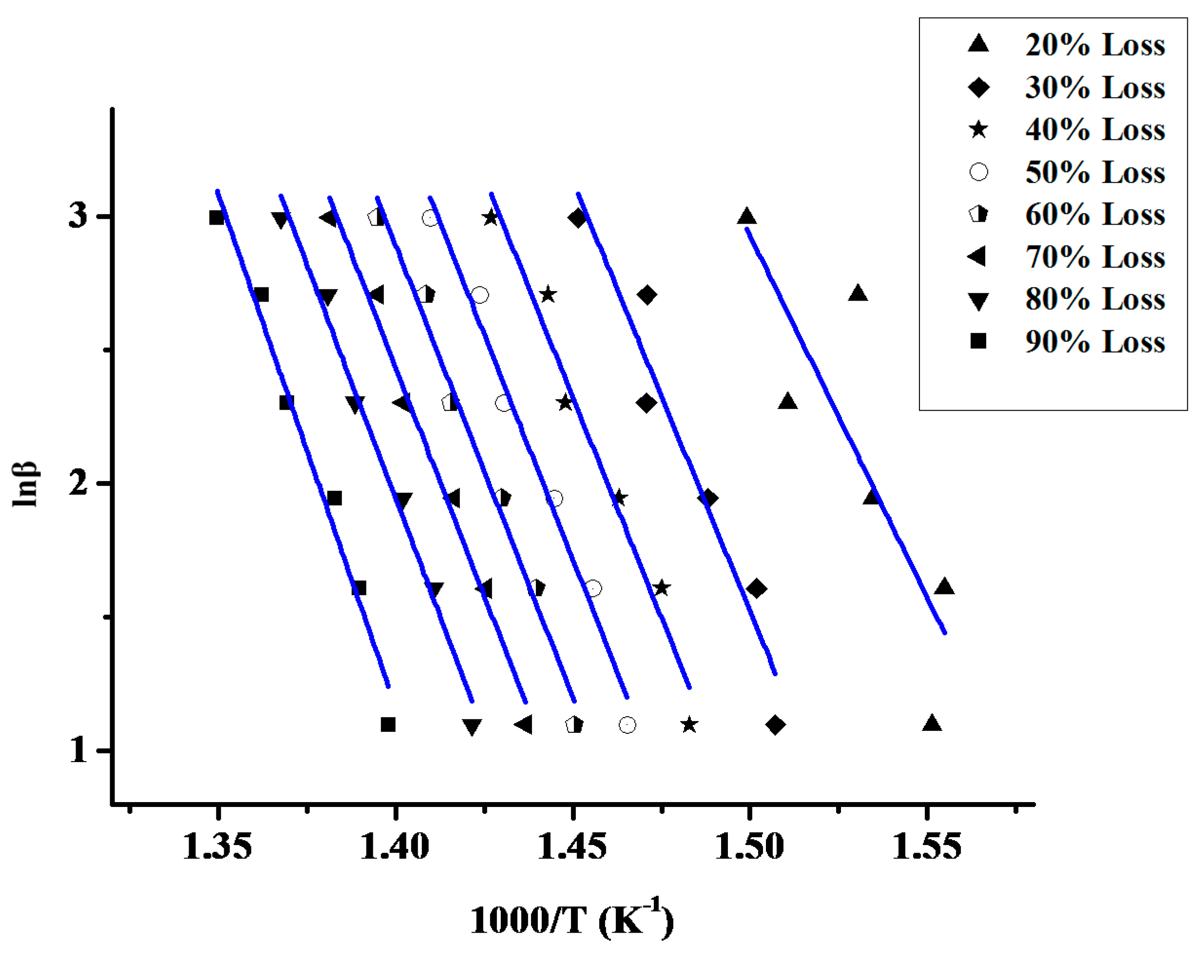
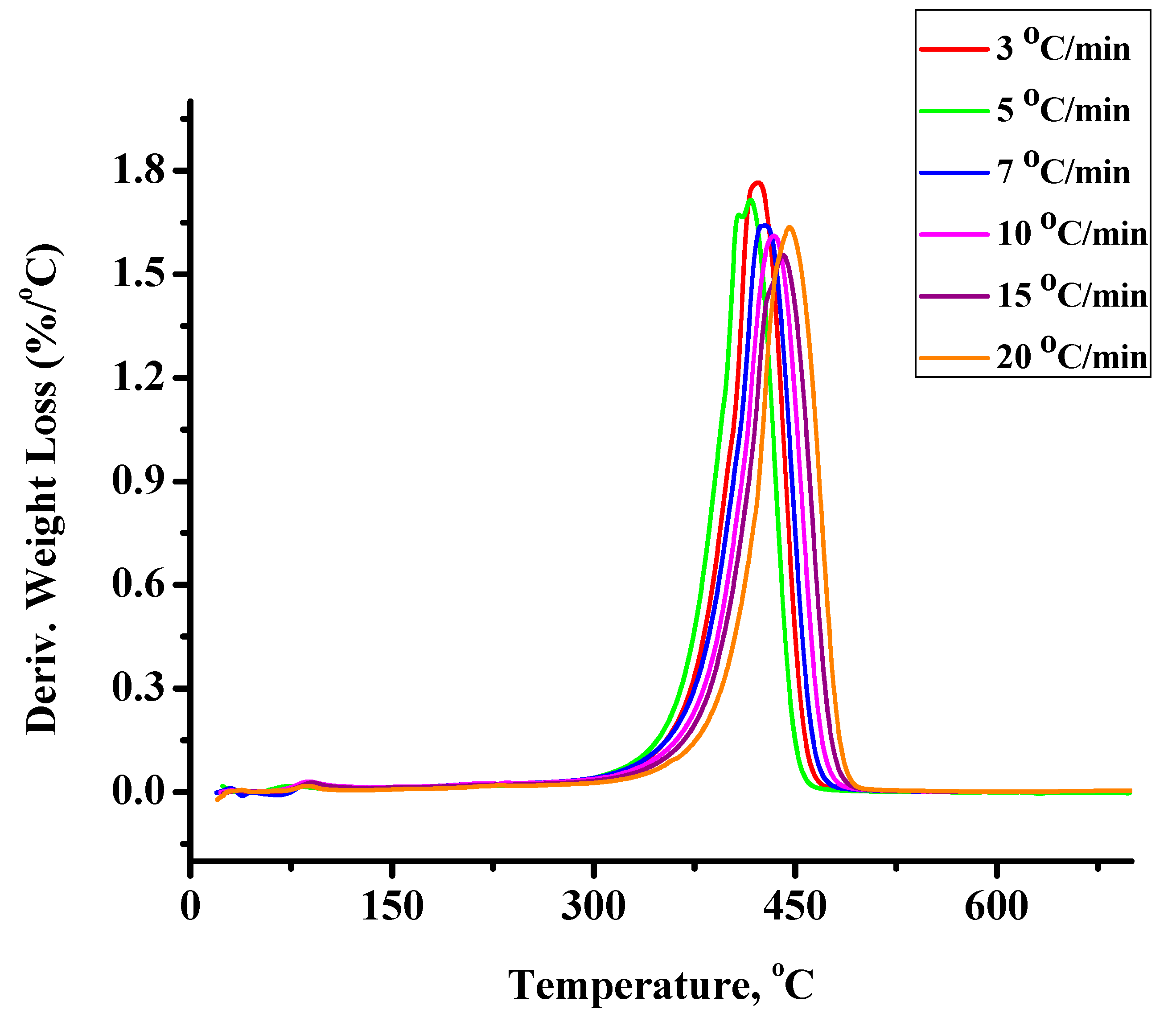
2.1.2. Kinetics of the Thermal Decomposition of the Statistical Copolymers


| Weight Loss | PCP | PNBE | 80/20 | 60/40 | 50/50 | 40/60 | 20/80 | 20/80P | 40/60P | 50/50P | 60/40P | 80/20P |
|---|---|---|---|---|---|---|---|---|---|---|---|---|
| 10 | 340.46 | - | 36.681 | 105.75 | - | 174.59 | - | 191.26 | 105.10 | - | - | - |
| 20 | 326.49 | - | 64.583 | 157.38 | - | 201.36 | 225.14 | 239.50 | 188.00 | 188.20 | - | - |
| 30 | 302.21 | - | 117.89 | 252.66 | 17.351 | 273.86 | 267.63 | 243.78 | 211.01 | 210.91 | 176.30 | 176.66 |
| 40 | 289.24 | 296.81 | 164.37 | 269.96 | 249.50 | 290.49 | 274.11 | 255.06 | 226.03 | 225.70 | 218.32 | 225.88 |
| 50 | 275.61 | 377.79 | 206.77 | 273.53 | 328.57 | 251.33 | 279.77 | 253.71 | 233.46 | 233.52 | 242.20 | 231.98 |
| 60 | 266.88 | 332.89 | 253.41 | 268.46 | 336.38 | 205.11 | 281.26 | 254.62 | 238.20 | 238.22 | 251.72 | 262.36 |
| 70 | 260.73 | 308.28 | 316.18 | 267.63 | 320.26 | 43.964 | 284.09 | 254.25 | 239.55 | 235.10 | 255.00 | 267.26 |
| 80 | 257.65 | - | 287.08 | 300.30 | 283.09 | 32.316 | 290.99 | 253.87 | 242.52 | 242.60 | 254.75 | 274.41 |
| 90 | 255.90 | - | 225.23 | - | 243.77 | - | 318.92 | 256.23 | 250.26 | 250.29 | 187.75 | 267.26 |
| Sample | Ea |
|---|---|
| PCP | 227.24 |
| PNBE | 247.11 |
| 20/80 | 190.30 |
| 40/60 | 214.21 |
| 50/50 | 316.54 |
| 60/40 | 214.49 |
| 80/20 | 275.64 |
| 20/80P | 253.69 |
| 40/60P | 249.55 |
| 50/50P | 243.62 |
| 60/40P | 236.62 |
| 80/20P | 259.13 |
2.2. Statistical Copolymers of NBE with CP in the Presence of Triphenylphosphine
2.2.1. Monomer Reactivity Ratios and Statistical Analysis of the Copolymers

2.2.2. Kinetics of the Thermal Decomposition of the Statistical Copolymers

3. Experimental Section
3.1. Materials
3.2. Copolymerization Studies
3.3. Copolymerization Reactions
3.4. Characterization Techniques
4. Conclusions
Supplementary Materials
Acknowledgments
Author Contributions
Conflicts of Interest
References
- Slugovc, C. The Ring Opening Metathesis Polymerisation Toolbox. Macromol. Rapid Commun. 2004, 25, 1283–1297. [Google Scholar] [CrossRef]
- Wiberg, K.B. The Concept of Strain in Organic Chemistry. Angew. Chem. Int. Ed. Engl. 1986, 25, 312–322. [Google Scholar] [CrossRef]
- Hérisson, J.L.; Chauvin, Y. Catalysis of olefin transformations by tungsten complexes. II. Telomerization of cyclic olefins in the presence of acyclic olefins. Makromol. Chem. 1971, 141, 161–176. [Google Scholar] [CrossRef]
- Katz, T.J.; McGinnis, J. Μechanism of the olefin metathesis reaction. J. Am. Chem. Soc. 1975, 97, 1592–1594. [Google Scholar] [CrossRef]
- Grubbs, R.H.; Burk, P.L.; Carr, D.D. Mechanism of the olefin metathesis reaction. J. Am. Chem. Soc. 1975, 97, 3265–3267. [Google Scholar]
- Katz, T.J.; Rothchild, R. Mechanism of the Olefin Metathesis of 2,2ʹ-Divinylbiphenyl. J. Am. Chem. Soc. 1976, 98, 2519–2526. [Google Scholar] [CrossRef]
- Grubbs, R.H.; Carr, D.D.; Hoppin, C.; Burk, P.L. Consideration of the mechanism of the metal catalyzed olefin metathesis reaction. J. Am. Chem. Soc. 1976, 98, 3478–3483. [Google Scholar] [CrossRef]
- Katz, T.J.; McGinnis, J. Metathesis of Cyclic and Acyclic Olefins. J. Am. Chem. Soc. 1977, 99, 1903–1912. [Google Scholar] [CrossRef]
- Leconte, M.; Basset, J.-M.; Quignard, F.; Larroche, C. Mechanistic Aspects of the Olefin Metathesis Reaction. In Reactions of Coordinated Ligands; Braterman, P.S., Ed.; Plenum: New York, NY, USA, 1986; Volume 1, pp. 371–420. [Google Scholar]
- Bielawski, C.W.; Grubbs, R.H. Living ring-opening metathesis polymerization. Prog. Polym. Sci. 2007, 32, 1–29. [Google Scholar] [CrossRef]
- Tirrell, D.A. Encyclopedia of Polymer Sciences and Engineering, 2nd ed.; Mark, H., Bikales, N.M., Overberger, C.G., Menges, G., Eds.; John Wiley & Sons: New York, NY, USA, 1985; Volume 4, p. 192. [Google Scholar]
- Zutty, L.; Faucher, J.A. The stiffness of ethylene copolymers. J. Polym. Sci. 1962, 60, S36–S37. [Google Scholar] [CrossRef]
- Stergiou, G.; Dousikos, P.; Pitsikalis, M. Radical copolymerization of styrene and alkyl methacrylates: Monomer reactivity ratios and thermal properties. Eur. Polym. J. 2002, 38, 1963–1970. [Google Scholar] [CrossRef]
- Makrikosta, G.; Georgas, D.; Siakali-Kioulafa, E.; Pitsikalis, M. Statistical copolymers of styrene and 2-vinylpyridine with trimethylsilyl methacrylate and trimethylsilyloxyethyl methacrylate. Eur. Polym. J. 2005, 41, 47–54. [Google Scholar] [CrossRef]
- Kostakis, Κ.; Mourmouris, S.; Kotakis, K.; Nikogeorgos, N.; Pitsikalis, M.; Hadjichristidis, N. Influence of the cocatalyst structure on the statistical copolymerization of methyl methacrylate with bulky methacrylates using the zirconocene complex Cp2ZrMe2. J. Polym. Sci. Polym. Chem. Ed. 2005, 43, 3305–3314. [Google Scholar]
- Kotzabasakis, V.; Petzetakis, N.; Pitsikalis, M.; Hadjichristidis, N.; Lohse, D.J. Copolymerization of tetradecene-1 and octene-1 with silyl-protected 10-undecen-1-ol using a Cs-symmetry hafnium metallocene catalyst. A route to functionalized poly(α-olefins). J. Polym. Sci. Polym. Chem. Ed. 2009, 47, 876–886. [Google Scholar] [CrossRef]
- Driva, P.; Bexis, P.; Pitsikalis, M. Radical Copolymerization of 2-Vinyl Pyridine and Oligo(Ethylene Glycol) Methyl Ether Methacrylates: Monomer Reactivity Ratios and Thermal Properties. Eur. Polym. J. 2011, 47, 762–771. [Google Scholar] [CrossRef]
- Droulia, M.; Anastasaki, A.; Rokotas, A.; Pitsikalis, M.; Paraskevopoulou, P. Statistical Copolymers of Methyl Methacrylate and 2-Methacryloyloxyethyl ferrocenecarboxylate: Monomer Reactivity Ratios, Thermal and Electrochemical Properties. J. Polym. Sci. Polym. Chem. Ed. 2011, 49, 3080–3089. [Google Scholar] [CrossRef]
- Karra, E.; Petrakou, I.; Driva, P.; Pitsikalis, M. Radical Copolymerization of 2-Vinyl Pyridine with Functional Methacrylates: Monomer Reactivity Ratios and Thermal Properties. Macromolecules 2013, 9, 68–77. [Google Scholar]
- Floros, G.; Agrafioti, F.; Grigoropoulos, A.; Paraskevopoulou, P.; Mertis, K.; Tseklima, M.; Veli, M.; Pitsikalis, M. Statistical copolymers of norbornene and 5-vinyl-2-norbornene by a ditungsten complex mediated ring opening metathesis polymerization. Synthesis, thermal properties and kinetics of thermal decomposition. J. Polym. Sci. Part A Polym. Chem. 2013, 51, 4835–4844. [Google Scholar] [CrossRef]
- Flory, P.J. Principles of Polymer Chemistry; Cornell University Press: Ithaca, NY, USA, 1953. [Google Scholar]
- Odian, G. Principles of Polymerization, 3rd ed.; Wiley Interscience: New York, NJ, USA, 1991. [Google Scholar]
- Ivin, K.J.; Mol, J.C. (Eds.) Olefin Metathesis and Metathesis Polymerization; Academic Press, Inc.: San Diego, CA, USA, 1997.
- Dragutan, V.; Streck, R. (Eds.) Catalytic Polymerization of Cycloolefins. Ionic, Ziegler-Natta and Ring-Opening Metathesis Polymerization; Elsevier Science B.V.: Amsterdam, The Netherlands, 2000.
- Grubbs, R.H. (Ed.) Handbook of Metathesis; Wiley-VCH: Weinheim, Germany, 2003.
- Frenzel, U.; Müller, B.K.M.; Nuyken, O. Handbook of Polymer Synthesis, 2nd ed.; Kricheldorf, H.R., Nuyken, O., Swift, G., Eds.; Marcel Dekker: New York, NY, USA, 2005. [Google Scholar]
- Buchmeiser, M.R. Homogeneous Metathesis Polymerization by Well-Defined Group VI and Group VIII Transition-Metal Alkylidenes: Fundamentals and Applications in the Preparation of Advanced Materials. Chem. Rev. 2000, 100, 1565–1604. [Google Scholar] [CrossRef] [PubMed]
- Buchmeiser, M.R. Synthesis of Polymers: New structures and Methods, 1st ed.; Schlüter, A.D., Hawker, C.J., Sakamoto, J., Eds.; Wiley-VCH: Weinheim, Germany, 2012. [Google Scholar]
- Myers, S.B.; Register, R.A. Synthesis of narrow-distribution polycyclopentene using a ruthenium ring-opening metathesis initiator. Polymer 2008, 49, 877–882. [Google Scholar] [CrossRef]
- Amir-Ebrahimi, V.; Corry, D.A.; Hamilton, J.G.; Thompson, J.M.; Rooney, J.J. Characteristics of RuCl2(CHPh)(PCy3)2 as a Catalyst for Ring-Opening Metathesis Polymerization. Macromolecules 2000, 33, 717–724. [Google Scholar] [CrossRef]
- Vougioukalakis, G.C.; Grubbs, R.H. Ruthenium-based heterocyclic carbene-coordinated olefin metathesis catalysts. Chem. Rev. 2010, 110, 1746–1787. [Google Scholar] [CrossRef] [PubMed]
- Sanford, M.S.; Ulman, M.; Grubbs, R.H. New Insights into the Mechanism of Ruthenium-Catalyzed Olefin Metathesis Reactions. J. Am. Chem. Soc. 2001, 123, 749–750. [Google Scholar] [CrossRef] [PubMed]
- Bielawski, C.W.; Grubbs, R.H. Increasing the Initiation Efficiency of Ruthenium-Based Ring-Opening Metathesis Initiators: Effect of Excess Phosphine. Macromolecules 2001, 34, 8838–8840. [Google Scholar] [CrossRef]
- Ivin, K.J.; O’Donnell, J.H.; Rooney, J.J.; Stewart, C.D. The 13C-NMR spectra of ring-opened copolymers of cyclopentene and norbornene; reactivity ratios. Makromol. Chem. 1979, 180, 1975–1988. [Google Scholar] [CrossRef]
- Porri, L.; Rossi, R.; Diversi, P.; Lucherini, A. Ring-opening polymerization of cycloolefins with catalysts derived from ruthenium and iridium. Die Makromol. Chem. 1974, 175, 3097–3115. [Google Scholar] [CrossRef]
- Ivin, K.J.; Lapienis, G.; Rooney, J.J. Ring-opening copolymerization of cycloalkenes investigated by 13C-NMR spectroscopy. Makromol. Chem. 1982, 183, 9–28. [Google Scholar] [CrossRef]
- Amir-Ebrahimi, V.; Rooney, J.J. Remarkable alternating effect in metathesis copolymerization of norbornene and cyclopentene using modified Grubbs ruthenium initiators. J. Mol. Catal. A Chem. 2004, 208, 115–121. [Google Scholar] [CrossRef]
- Amir-Ebrahimi; Carvill, A.G.; Hamilton, J.G.V.; Rooney, J.J.; Tuffy, C. Copolymerization of cycloalkenes as a probe of the propagation steps in olefin metathesis. J. Mol. Catal. A Chem. 1997, 115, 85–94. [Google Scholar] [CrossRef]
- Gallagher, M.M.; Rooney, A.D.; Rooney, J.J. Metathesis co-polymerization as a means of comparing the reactivity of ruthenium initiators in conventional solvents and ionic liquids. J. Mol. Catal. A Chem. 2009, 303, 78–83. [Google Scholar] [CrossRef]
- Vehlow, K.; Lichtenheldt, M.; Wang, D.; Blechert, S.; Buchmeiser, M.R. Alternating ring-opening copolymerization of norborn-2-ene with cis-cyclooctene and cyclopentene. Macromol. Symp. 2010, 296, 44–48. [Google Scholar] [CrossRef]
- Buchmeiser, M.R.; Ahmad, I.; Gurram, V.; Kumar, P.S. Pseudo-Halide and Nitrate Derivatives of Grubbs and Grubbs-Hoveyda Initiators: Some Structural Features Related to the Alternating Ring-Opening Metathesis Copolymerization of Norborn-2-ene with Cyclic Olefins. Macromolecules 2011, 44, 4098–4106. [Google Scholar] [CrossRef]
- Fineman, M.; Ross, S. Linear method for determining monomer reactivity ratios in copolymerization. J. Polym. Sci. 1950, 5, 259–262. [Google Scholar] [CrossRef]
- Kelen, T.; Tüdos, F. Analysis of the Linear Methods for Determining Copolymerization Reactivity Ratios. I. A New Improved Linear Graphic Method. J. Macromol. Sci. A 1975, 9. [Google Scholar] [CrossRef]
- Beginn, U. COPOINT a simple computer program to determine copolymerization parameters by numerical integration. e-Polymers 2005, 73, 759–782. [Google Scholar] [CrossRef]
- Krause, J.O.; Wurst, K.; Nuyken, O.; Buchmeiser, M.R. Synthesis and Reactivity of Homogeneous and Heterogeneous Ruthenium-Based Metathesis Catalysts Containing Electron-Withdrawing Ligands. Chem. Eur. J. 2004, 10, 777–784. [Google Scholar] [CrossRef] [PubMed]
- Kumar, P.S.; Buchmeiser, M.R. Ru-Alkylidene Metathesis Catalysts Based on 1,3-Dimesityl-4,5,6,7-tetrahydro-1,3-diazepin-2-ylidenes: Synthesis, Structure, and Activity. Organometallics 2009, 28, 1785–1790. [Google Scholar] [CrossRef]
- Conrad, J.C.; Camm, K.D.; Fogg, D.E. Ru-Aryloxide Metathesis Catalysts with Enhanced Lability. Inorg. Chim. Acta 2006, 359, 1967–1974. [Google Scholar] [CrossRef]
- Dinger, M.B.; Nieczypor, P.; Mol, J.C. Adamantyl-Substituted N-Heterocyclic Carbene Ligands in Second-Generation Grubbs-Type Metathesis Catalysts. Organometallics 2003, 22, 5291–5296. [Google Scholar] [CrossRef]
- Dereli, O.; Düz, B.; İmamoğlu, Y. The WCl6–e−–Al–CH2Cl2 catalyzed polypentenamer formation via ring-opening metathesis polymerization (ROMP). Eur. Polym. J. 2006, 42, 368–374. [Google Scholar] [CrossRef]
- Naga, N.; Kikuchi, G.; Toyota, A. Synthesis and crystalline structure of polyethylene containing 1,3-cylopentane units in the main chain by ring-opening metathesis copolymerization of cycloolefins following hydrogenation reaction. Polymer 2006, 47, 6081–6090. [Google Scholar] [CrossRef]
- Hiemenz, P.C. Polymer Chemistry; The Basic Concepts, Marcel Dekker Inc.: New York, NY, USA, 1984. [Google Scholar]
- Igarashi, S. Representation of composition and blockiness of the copolymer by a triangular coordinate system. J. Polym. Sci. Polym. Lett. Ed. 1963, 1, 359–363. [Google Scholar] [CrossRef]
- Elias, H.G. Macromolecules; Plenum Press: New York, NY, USA; London, UK, 1971; Volume 2, Chapter 22; p. 761. [Google Scholar]
- Ozawa, T. A New Method of Analyzing Thermogravimetric Data. Bull. Chem. Soc. Jpn. 1965, 38, 1881–1886. [Google Scholar] [CrossRef]
- Flynn, J.; Wall, L.A. A quick, direct method for the determination of activation energy from thermogravimetric data. J. Polym. Sci. Part B Polym. Lett. 1966, 4, 323–328. [Google Scholar] [CrossRef]
- Ozawa, T. Kinetic analysis of derivative curves in thermal analysis. J. Therm. Anal. Calorim. 1970, 2, 301–324. [Google Scholar] [CrossRef]
- Kissinger, H.E. Variation of Peak Temperature with Heating Rate in Differential Thermal Analysis. J. Res. Nat. Bur. Stand. 1956, 57, 217–221. [Google Scholar] [CrossRef]
- Kissinger, H.E. Reaction kinetic in differential thermal analysis. Anal. Chem. 1957, 29, 1702–1712. [Google Scholar] [CrossRef]
- Lee, L.B.W.; Register, R.A. Acyclic metathesis during ring-opening metathesis polymerization of cyclopentene. Polymer 2004, 45, 6479–6485. [Google Scholar] [CrossRef]
- Sample Availability: Samples of the copolymers are available from the authors.
© 2015 by the authors. Licensee MDPI, Basel, Switzerland. This article is an open access article distributed under the terms and conditions of the Creative Commons Attribution license ( http://creativecommons.org/licenses/by/4.0/).
Share and Cite
Nikovia, C.; Maroudas, A.-P.; Goulis, P.; Tzimis, D.; Paraskevopoulou, P.; Pitsikalis, M. Statistical Ring Opening Metathesis Copolymerization of Norbornene and Cyclopentene by Grubbs’ 1st-Generation Catalyst. Molecules 2015, 20, 15597-15615. https://doi.org/10.3390/molecules200915597
Nikovia C, Maroudas A-P, Goulis P, Tzimis D, Paraskevopoulou P, Pitsikalis M. Statistical Ring Opening Metathesis Copolymerization of Norbornene and Cyclopentene by Grubbs’ 1st-Generation Catalyst. Molecules. 2015; 20(9):15597-15615. https://doi.org/10.3390/molecules200915597
Chicago/Turabian StyleNikovia, Christiana, Andreas-Philippos Maroudas, Panagiotis Goulis, Dionysios Tzimis, Patrina Paraskevopoulou, and Marinos Pitsikalis. 2015. "Statistical Ring Opening Metathesis Copolymerization of Norbornene and Cyclopentene by Grubbs’ 1st-Generation Catalyst" Molecules 20, no. 9: 15597-15615. https://doi.org/10.3390/molecules200915597
APA StyleNikovia, C., Maroudas, A.-P., Goulis, P., Tzimis, D., Paraskevopoulou, P., & Pitsikalis, M. (2015). Statistical Ring Opening Metathesis Copolymerization of Norbornene and Cyclopentene by Grubbs’ 1st-Generation Catalyst. Molecules, 20(9), 15597-15615. https://doi.org/10.3390/molecules200915597