
Hemodynamic Effects on Particle Targeting in the Arterial Bifurcation for Different Magnet Positions


Abstract
1. Introduction
2. Problem Description
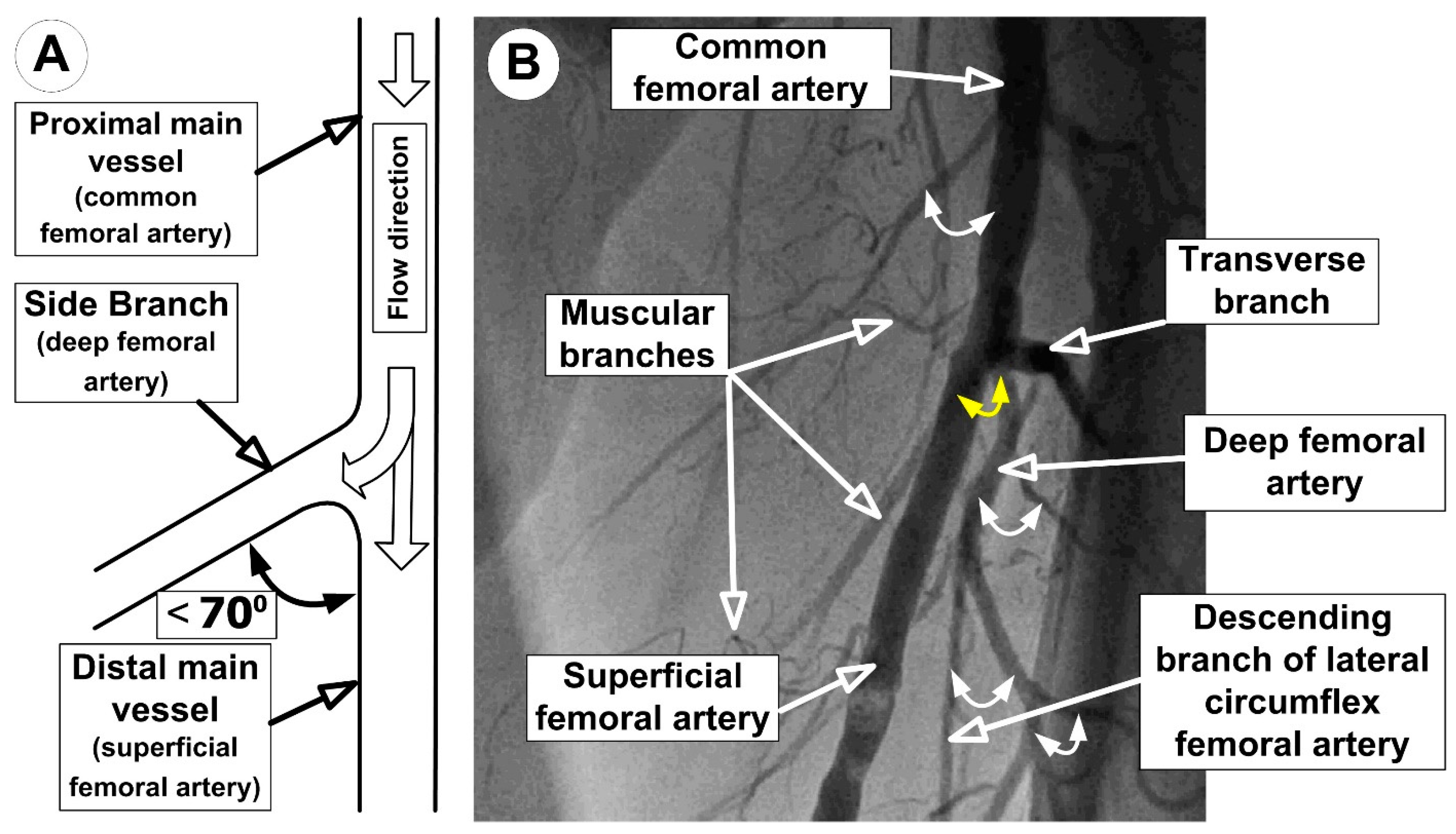
2.1. Investigated Arterial Bifurcation
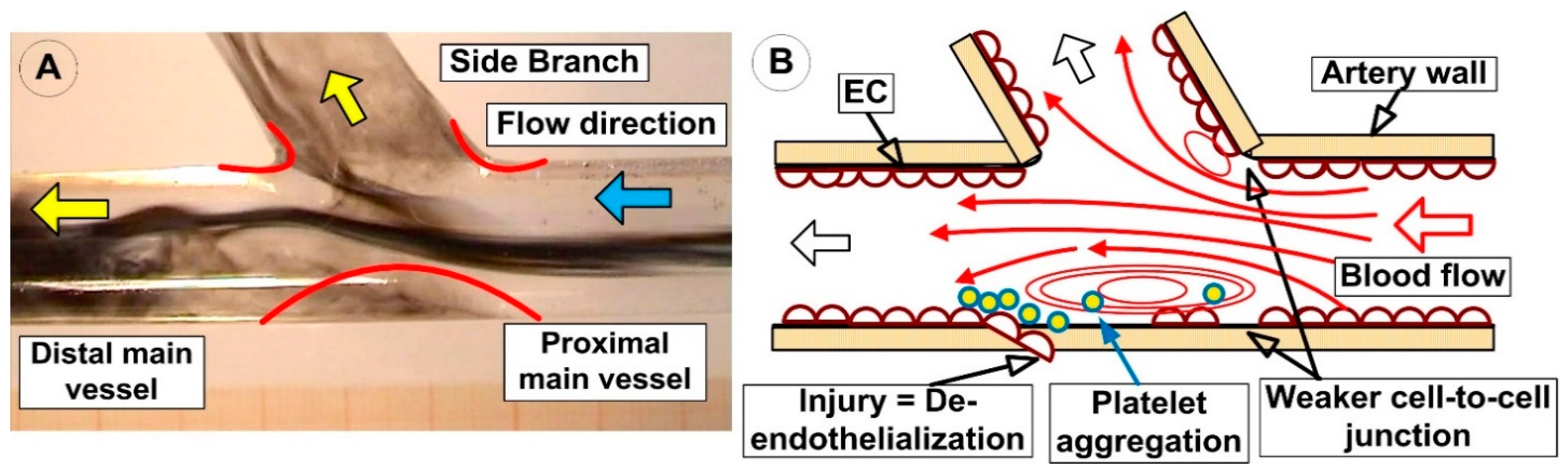
2.2. Arterial Bifurcation Lesion
2.3. Purpose of the Study
3. Materials and Method
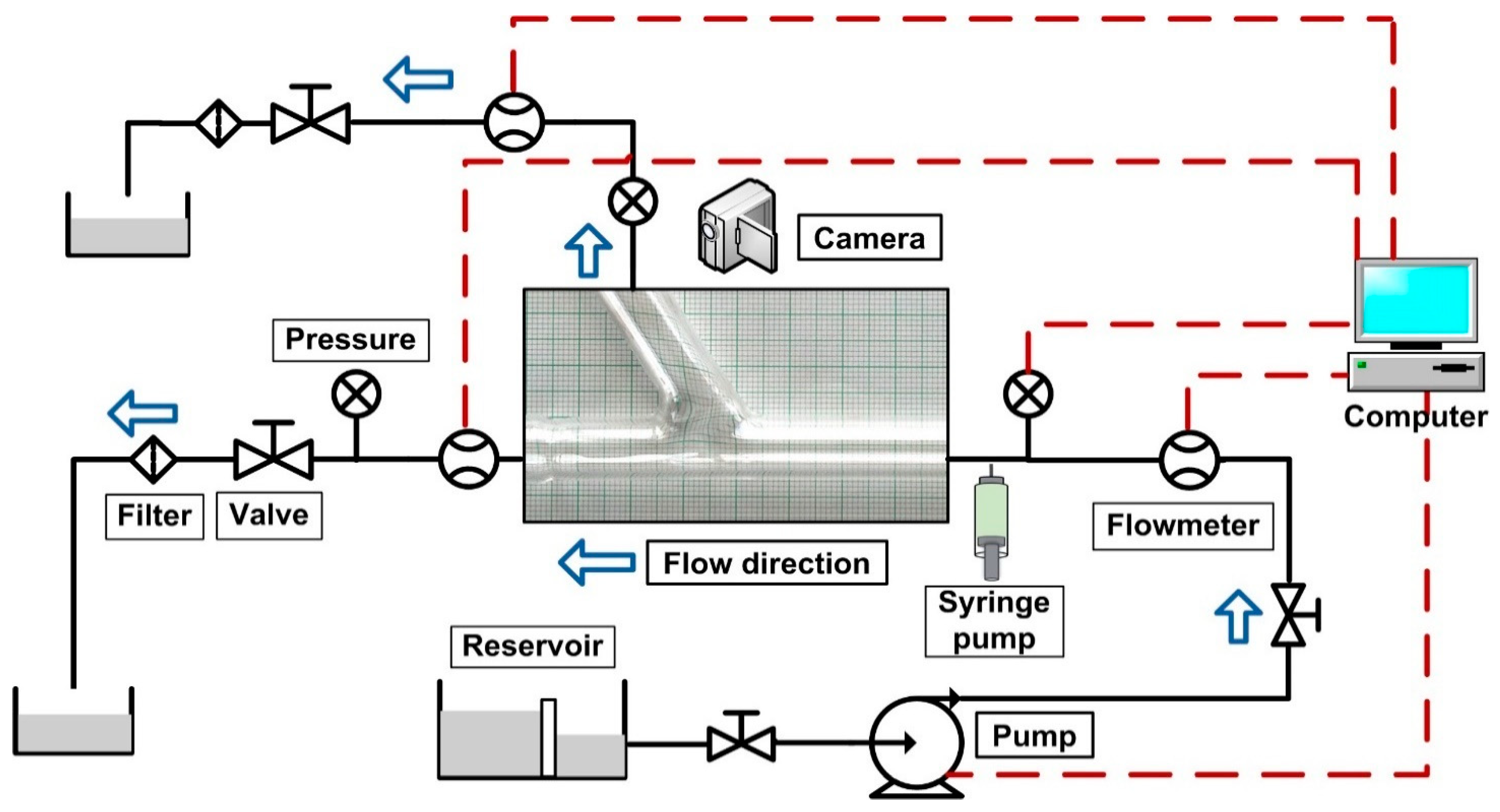
3.1. Experimental Test Rig
3.2. Experimental Bifurcation Geometry
3.3. Blood Analog Fluid Preparation
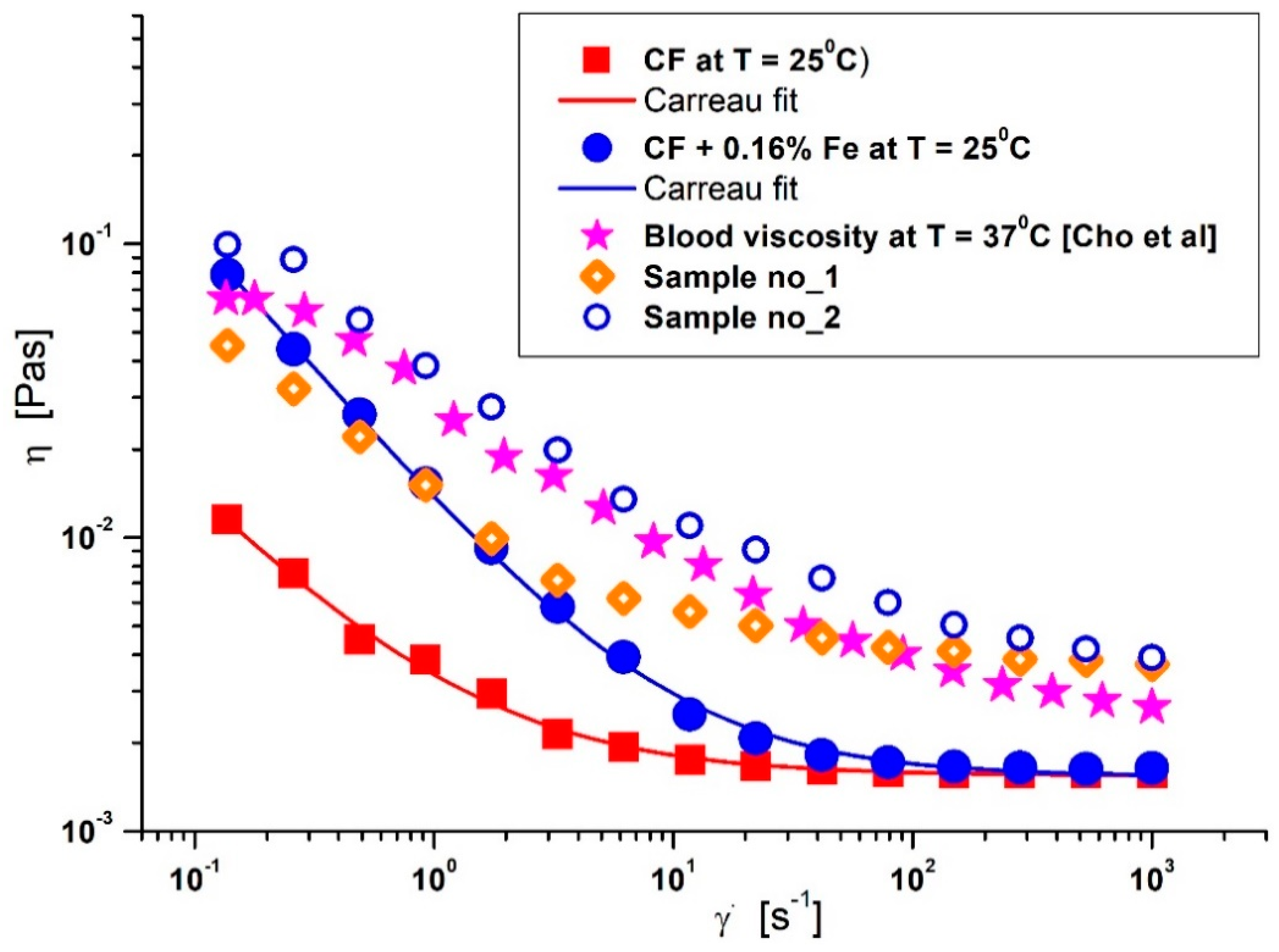
Rheological Properties of the Blood Analog Fluid
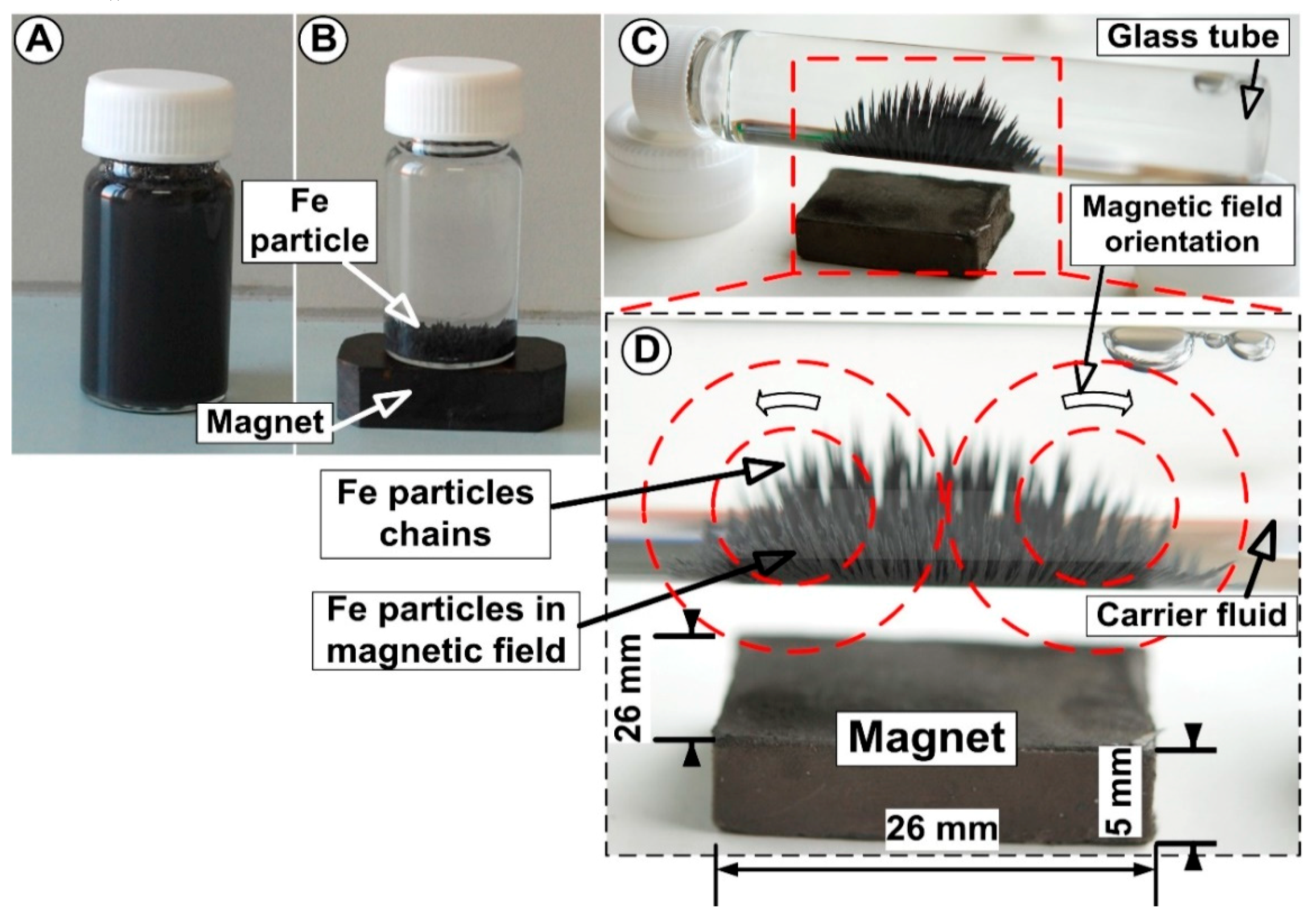
3.4. Magnetic Particle Characterization
3.5. Magnetic Field Generation
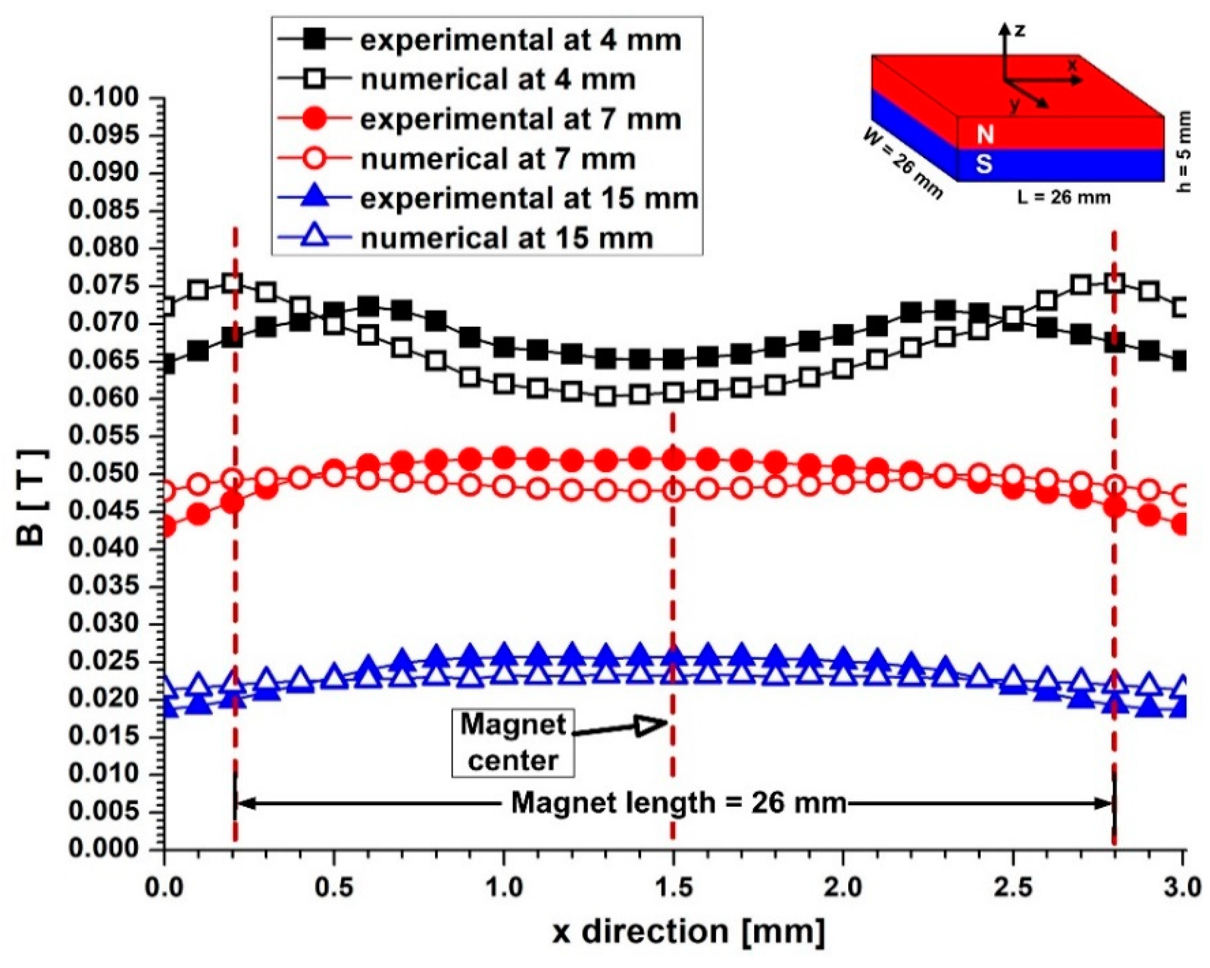
3.5.1. The Experimentally Measured Magnetic Field
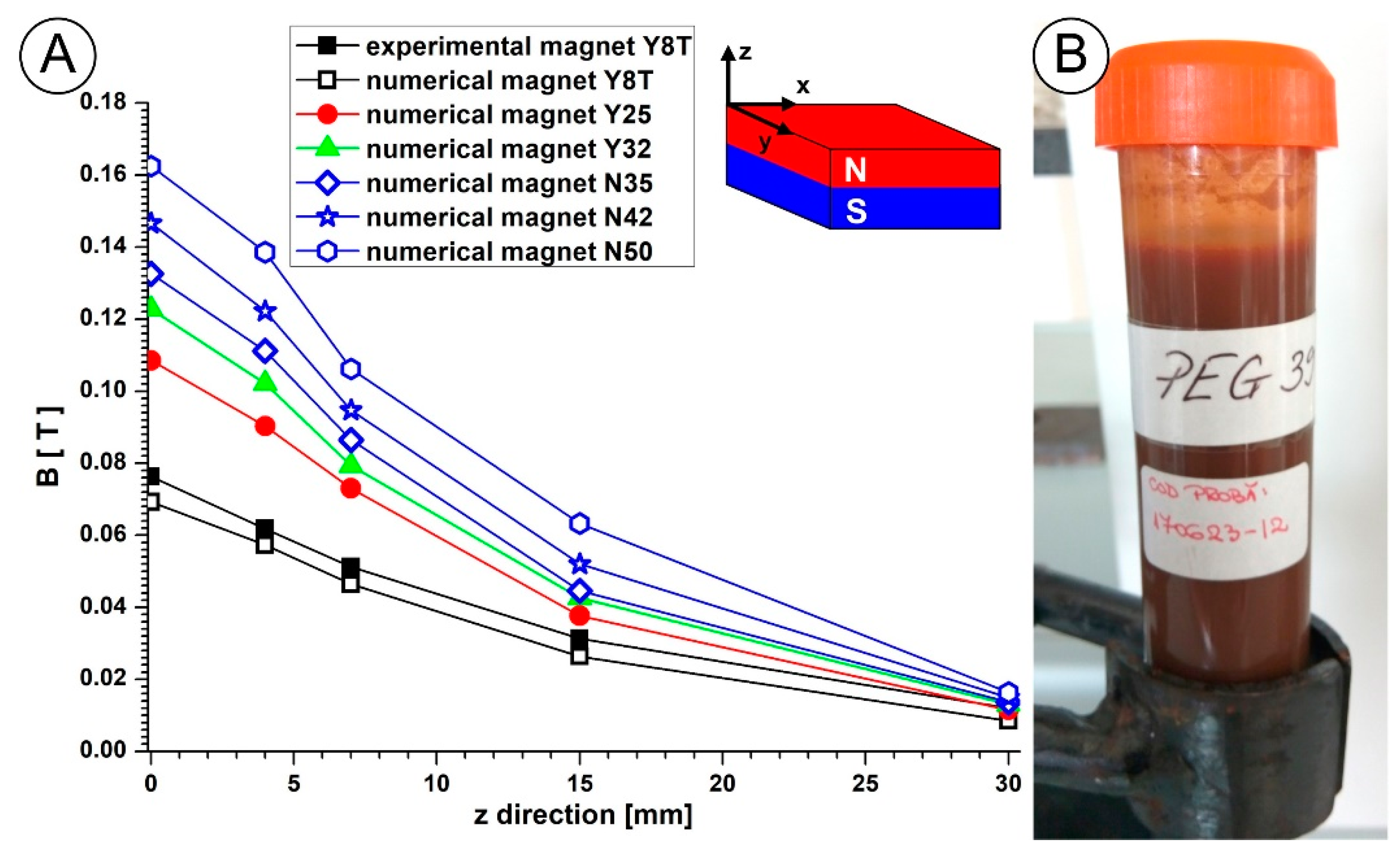
3.5.2. Numerical Investigation of the Magnetic Field
4. Results and Discussions
4.1. Bifurcation Hemodynamics
4.2. Experimental Magnetic Particle Deposition
4.2.1. Principles of the Magnetic Particle Deposition in the Arterial Bifurcation
4.2.2. Particle Deposition
4.3. Targeting Efficiency
4.4. Medical Importance
5. Conclusions
6. Future Steps
Supplementary Materials
Author Contributions
Funding
Acknowledgments
Conflicts of Interest
References
- Shishehbor, M.H.; Reed, G.W. Personalized approach to revascularization of critical limb ischemia. Circ. Cardiovasc. Interv. 2014, 7, 642–644. [Google Scholar] [CrossRef] [PubMed][Green Version]
- Lovell, M.; Dickson, C.; Lindsay, T.F. Peripheral artery disease: The unknown cardiovascular risk. Diabet. Foot Can. 2015, 3, 6–9. [Google Scholar]
- Klein, A.J.; Jaff, M.R.; Gray, B.H.; Aronow, H.D.; Bersin, R.M.; Diaz-Sandoval, L.J.; Dieter, R.S.; Drachman, D.E.; Feldman, D.N.; Gigliotti, O.S.; et al. SCAI appropriate use criteria for peripheral arterial interventions: An update. Catheter. Cardiovasc. Interv. 2017, E90–E110. [Google Scholar] [CrossRef] [PubMed]
- Wilkins, L.R.; Sabri, S.S. Strategies to approaching lower limb occlusions. Tech. Vasc. Interv. Radiol. 2016, 19, 136–144. [Google Scholar] [CrossRef] [PubMed]
- Foin, N.; Lee, R.D.; Torii, R.; Guitierrez-Chico, J.L.; Mattesini, A.; Nijjer, S.; Sen, S.; Petraco, R.; Davies, E.J.; Di Mario, C.; et al. Impact of stent strut design in metallic stents and biodegradable scaffolds. Int. J. Cardiol. 2014, 177, 800–808. [Google Scholar] [CrossRef] [PubMed]
- Otsuka, F.; Vorpahl, M.; Nakano, M.; Foerst, J.; Newell, J.B.; Sakakura, K.; Kutys, R.; Ladich, E.; Finn, A.V.; Kolodgie, F.K.; et al. Pathology of Second-Generation Everolimus-Eluting Stents Versus First-Generation Sirolimus- and Paclitaxel-Eluting Stents in Humans. Circulation 2014, 129, 211–223. [Google Scholar] [CrossRef] [PubMed]
- Pislaru, S.V.; Harbuzariu, A.; Gulati, R.; Witt, T.; Sandhu, M.P.; Simari, R.D.; Sandhu, G.S. Magnetically targeted endothelial cell localization in stented vessels. J. Am. Coll. Cardiol. 2006, 48, 1839–1845. [Google Scholar] [CrossRef] [PubMed]
- Polyak, B.; Fishbein, I.; Chorny, M.; Alferiev, I.; Williams, D.; Yellen, B.; Friedman, G.; Levy, R.J. High field gradient targeting of magnetic nanoparticle-loaded endothelial cells to the surfaces of steel stents. Proc. Natl. Acad. Sci. USA 2008, 105, 698–703. [Google Scholar] [CrossRef] [PubMed]
- Kyrtatos, P.G.; Lehtolainen, P.; Junemann-Ramirez, M.; Garcia-Prieto, A.; Price, A.N.; Martin, G.F.; Gadian, D.G.; Pankhurst, Q.A.; Lythgoe, M.F. Magnetic tagging increases delivery of circulating progenitors in vascular injury. Jacc Cardiovasc. Interv. 2009, 2, 794–802. [Google Scholar] [CrossRef] [PubMed]
- Gitter, K.; Odenbach, S. Quantitative targeting maps based on experimental investigations for a branched tube model in magnetic drug targeting. J. Magn. Magn. Mater. 2011, 323, 3038–3042. [Google Scholar] [CrossRef]
- Riegler, J.; Wells, J.A.; Kyrtatos, P.G.; Price, A.N.; Pankhurst, Q.A.; Lythgoe, M.F. Targeted magnetic delivery and tracking of cells using a magnetic resonance imaging system. Biomaterials 2010, 31, 5366–5371. [Google Scholar] [CrossRef] [PubMed]
- Mishima, F.; Takeda, S.I.; Izumi, Y.; Nishijima, S. Three Dimensional Motion Control System of Ferromagnetic Particles for Magnetically Targeted Drug Delivery Systems. IEEE Trans. Appl. Supercond. 2006, 16, 1539–1542. [Google Scholar] [CrossRef]
- Matuszaka, J.; Zaloga, J.; Friedrich, R.P.; Lyer, S.; Nowak, J.; Odenbach, S.; Alexiou, C.; Cicha, I. Endothelial biocompatibility and accumulation of SPION under flow conditions. J. Magn. Magn. Mater. 2015, 380, 20–26. [Google Scholar] [CrossRef]
- Weddell, J.C.; Kwack, J.; Imoukhuede, P.I.; Masud, A. Hemodynamic Analysis in an Idealized Artery Tree: Differences in Wall Shear Stress between Newtonian and Non-Newtonian Blood Models. PLoS ONE 2015, 10, e0124575. [Google Scholar] [CrossRef] [PubMed]
- Blanco, P.G.; Watanabe, S.M.; Passos, M.A.R.F.; Lemos, P.A.; Feijoo, R.A. An Anatomically Detailed Arterial Network Model for One-Dimensional Computational Hemodynamics. IEEE Trans. Biomed. Eng. 2015, 62, 736–753. [Google Scholar] [CrossRef] [PubMed]
- Chen, Y.; Deng, K.; Xiong, Y.; Jiang, W.; Wang, G.; Fan, Y. Numerical simulation on the effects of drug release positions in hepatic portal vein for targeting therapy. J. Mech. Med. Biol. 2015, 15, 1550038. [Google Scholar] [CrossRef]
- Gitter, K.; Odenbach, S. Investigations on a Branched Tube Model in Magnetic Drug Targeting—Systematic Measurements and Simulation. IEEE Trans. Magn. 2013, 49, 343–348. [Google Scholar] [CrossRef]
- Pakravan, H.A.; Saidi, M.S.; Firoozabadi, B. FSI simulation of a healthy coronary bifurcation for studying the mechanical stimuli of endothelial cells under different physiological conditions. J. Mech. Med. Biol. 2015, 15, 1550089. [Google Scholar] [CrossRef]
- Otero-Cacho, A.; Aymerich, M.; Flores-Arias, M.T.; Abal, M.; Álvarez, E.; Pérez-Muñuzuri, V.; Muñuzuri, A.P. Determination of hemodynamic risk for vascular disease in planar artery bifurcations. Sci. Rep. 2018, 8, 2795. [Google Scholar] [CrossRef]
- Kong, F.Y.; Zhang, J.W.; Li, R.F.; Wang, Z.X.; Wang, W.J.; Wang, W. Unique Roles of Gold Nanoparticles in Drug Delivery, Targeting and Imaging Applications. Molecules 2017, 22, 1445. [Google Scholar]
- Hornung, A.; Poettler, M.; Friedrich, R.P.; Zaloga, J.; Unterweger, H.; Lyer, S.; Nowak, J.; Odenbach, S.; Alexiou, C.; Janko, C. Treatment Efficiency of Free and Nanoparticle-Loaded Mitoxantrone for Magnetic Drug Targeting in Multicellular Tumor Spheroids. Molecules 2015, 20, 18016–18030. [Google Scholar] [CrossRef] [PubMed]
- Cicha, I.; Chauvierre, C.; Texier, I.; Cabella, C.; Metselaar, J.M.; Szebeni, J.; Dézsi, L.; Alexiou, C.; Rouzet, F.; Storm, G.; et al. From design to the clinic: Practical guidelines for translating cardiovascular nanomedicine. Cardiovasc. Res. 2018, 114, 1714–1727. [Google Scholar] [CrossRef] [PubMed]
- Dézsi, L.; Szénási, G.; Urbanics, R.; Rosivall, L.; Szebeni, J. Cardiopulmonary and hemodynamic changes in complement activation-related pseudoallergy. Health 2013, 5, 1032–1038. [Google Scholar]
- Lefevre, T.; Louvard, Y.; Morice, M.C.; Dumas, P.; Loubeyre, C.; Benslimane, A.; Premchand, R.K.; Guillard, N.; Piéchaud, J.-F. Stenting of bifurcation lesions: Classification, treatments, and results. Catheter. Cardiovasc. Interv. 2000, 49, 274–283. [Google Scholar] [CrossRef]
- Radegran, G.; Saltin, B. Human femoral artery diameter in relation to knee extensor muscle mass, peak blood flow, and oxygen uptake. Am. J. Physiol. Heart Circ. Physiol. 2000, 278, H162–H167. [Google Scholar] [CrossRef] [PubMed]
- Sandgren, T.; Sonesson, B.; Ahlgren, A.R.; Länne, T. The diameter of the common femoral artery in healthy human: Influence of sex, age, and body size. J. Vasc. Surg. 1999, 29, 503–510. [Google Scholar] [CrossRef]
- Moore, E.J.; Timmins, H.L.; LaDisa, J.F., Jr. Coronary Artery Bifurcation Biomechanics and Implications for Interventional Strategies. Catheter. Cardiovasc. Interv. 2010, 76, 836–843. [Google Scholar] [CrossRef]
- Kelly, M.; Yeoh, G.H.; Timchenko, V. On Computational Fluid Dynamics Study of Magnetic Drug Targeting. J. Comput. Multiphase Flows 2015, 7, 43–56. [Google Scholar] [CrossRef][Green Version]
- Eckstein, E.C.; Tilles, A.W.; Millero, F.J., III. Conditions for the occurrence of large near-wall excesses of small particles during blood flow. Microvasc. Res. 1988, 36, 31–39. [Google Scholar] [CrossRef]
- Abkarian, M.; Lartigue, C.; Viallat, A. Tank treading and unbinding of deformable vesicles in shear flow: Determination of the lift force. Phys. Rev. Lett. 2002, 88, 068103. [Google Scholar] [CrossRef]
- Kumar, A.; Graham, M.D. Mechanism of margination in confined flows of blood and other multicomponent suspensions. Phys. Rev. Lett. 2012, 109, 108102. [Google Scholar] [CrossRef] [PubMed]
- Muller, K.; Fedosov, D.A.; Gompper, G. Margination of micro- and nano-particles in blood flow and its effect on drug Delivery. Sci. Rep. 2015, 4, 4871. [Google Scholar] [CrossRef] [PubMed]
- Watts, T.; Barigou, M.; Nash, G.B. Comparative rheology of the adhesion of platelets and leukocytes from flowing blood: Why are platelets so small? Am. J. Physiol. Heart. Circ. Physiol. 2013, 304, H1483–H1494. [Google Scholar] [CrossRef] [PubMed]
- Bernad, S.I.; Totorean, A.F.; Vekas, L. Particles deposition induced by the magnetic field in the coronary bypass graft model. J. Magn. Magn. Mater. 2016, 401, 269–286. [Google Scholar] [CrossRef]
- Chen, H.; Kaminski, M.D.; Pytel, P.; Macdonald, L.; Rosengart, A.J. Capture of magnetic carriers within large arteries using external magnetic fields. J. Drug Target. 2008, 16, 262–268. [Google Scholar] [CrossRef] [PubMed]
- Galanzha, E.I.; Shashkov, E.V.; Kelly, T.; Kim, J.W.; Yang, L.; Zharov, V.P. In vivo magnetic enrichment and multiplex photoacoustic detection of circulating tumour cells. Nat. Nanotechnol. 2009, 4, 855–860. [Google Scholar] [CrossRef] [PubMed]
- Sugioka, T.; Ochi, M.; Yasunaga, Y.; Adachi, N.; Yanada, S. Accumulation of magnetically labeled rat mesenchymal stem cells using an external magnetic force, and their potential for bone regeneration. J. Biomed. Mater. Res. A 2008, 85, 597–604. [Google Scholar] [CrossRef]
- Holland, C.K.; Brown, J.M.; Scoutt, L.M.; Taylor, K.J.W. Lower extremity volumetric arterial blood flow in normal subjects. Ultrasound Med. Biol. 1998, 24, 1079–1086. [Google Scholar] [CrossRef]
- Meier, P.; Brilakis, E.S.; Corti, R.; Knapp, G.; Shishehbor, M.H.; Gurn, H.S. Drug-eluting versus bare-metal stent for treatment of saphenous vein grafts: A meta-analysis. PLoS ONE 2010, 5, e11040. [Google Scholar] [CrossRef]
- Pislaru, S.V.; Harbuzariu, A.; Agarwal, G.; Witt, T.; Gulati, R.; Sandhu, N.P.; Mueske, C.; Kalra, M.; Simari, R.D.; Sandhu, G.S. Magnetic forces enable rapid endothelialization of synthetic vascular grafts. Circulation 2006, 114, I-314–I-318. [Google Scholar] [CrossRef]
- Cho, Y.I.; Kensey, K.R. Effects of the non-Newtonian viscosity of blood on flows in a diseased arterial vessel. Part 1: Steady flows. Biorheology 1991, 28, 241–262. [Google Scholar] [CrossRef]
- Bernad, S.I.; Susan-Resiga, D.; Vekas, L.; Bernad, E.S. Drug targeting investigation in the critical region of the arterial bypass graft. J. Magn. Magn. Mater. 2019, 475, 14–23. [Google Scholar] [CrossRef]
- Mezger, T.G. The Rheology Handbook; Curt, R., Ed.; Vincentz Verlag: Hannover, Germany, 2002. [Google Scholar]
- Susan-Resiga, D.; Bica, D.; Vekas, L. Flow behavior of extremly bidisperse magnetizable fluids. J. Magn. Magn. Mater. 2010, 322, 3166–3172. [Google Scholar] [CrossRef]
- Laurent, S.; Saei, A.A.; Behzadi, S.; Panahifar, A.; Mahmoudi, M. Superparamagnetic iron oxide nanoparticles for delivery of therapeutic agents: Opportunities and challenges. Expert Opin. Drug Deliv. 2014, 11, 1–22. [Google Scholar] [CrossRef] [PubMed]
- Reddy, L.H.; Arias, J.L.; Nicolas, J.; Couvreur, P. Magnetic Nanoparticles: Design and Characterization, Toxicity and Biocompatibility, Pharmaceutical and Biomedical Applications. Chem. Rev. 2012, 112, 5818–5878. [Google Scholar] [CrossRef] [PubMed]
- Goodwin, S.C.; Bittner, C.A.; Peterson, C.L.; Wong, G. Single-dose toxicity study of hepatic intra-arterial infusion of doxorubicin coupled to a novel magnetically targeted drug carrier. Toxicol. Sci. 2001, 60, 177–183. [Google Scholar] [CrossRef] [PubMed]
- Nacev, A.; Beni, C.; Bruno, O.; Shapiro, B. The behaviors of ferromagnetic nano-particles in and around blood vessels under applied magnetic fields. J. Magn. Magn. Mater. 2011, 323, 651–668. [Google Scholar] [CrossRef]
- Ta, H.T.; Truong, N.P.; Whittaker, A.K.; Davis, T.P.; Karlheinz, P. The effects of particle size, shape, density and flow characteristics on particle margination to vascular walls in cardiovascular diseases. Expert Opin. Drug Deliv. 2017. [Google Scholar] [CrossRef]
- Cores, J.; Caranasos, T.G.; Cheng, K. Magnetically targeted stem cell delivery for regenerative medicine. J. Funct. Biomater. 2015, 6, 526–546. [Google Scholar] [CrossRef]
- Connell, J.J.; Patrick, S.P.; Yu, Y.; Lythgoe, M.F.; Kalber, T.L. Advanced cell therapies: Targeting, tracking and actuation of cells with magnetic particles. Regen. Med. 2015, 10, 757–772. [Google Scholar] [CrossRef]
- Mahmoud, E.E.; Kamei, G.; Harada, Y.; Shimizu, R.; Kamei, N.; Adachi, N.; Misk, N.A.; Ochi, M. Cell magnetic targeting system for repair of severe chronic osteochondral defect in a rabbit model. Cell Transpl. 2016, 25, 1073–1083. [Google Scholar] [CrossRef]
- Kamei, G.; Kobayashi, T.; Ohkawa, S.; Kongcharoensombat, W.; Adachi, N.; Takazawa, K.; Shibuya, H.; Deie, M.; Hattori, K.; Goldberg, J.L.; et al. Articular cartilage repair with magnetic mesenchymal stem cells. Am. J. Sports Med. 2013, 41, 1255–1264. [Google Scholar] [CrossRef] [PubMed]
- Riegler, J.; Lau, K.D.; Garcia-Prieto, A.; Price, A.N.; Richards, T.; Pankhurst, Q.A.; Lythgoe, M.F. Magnetic cell delivery for peripheral arterial disease: A theoretical framework. Med. Phys. 2011, 38, 3932–3943. [Google Scholar] [CrossRef] [PubMed]
- Meng, H.; Wang, Z.; Hoi, Y.; Gao, L.; Metaxa, E.; Swartz, D.D.; Kolega, J. Complex Hemodynamics at the Apex of an Arterial Bifurcation Induces Vascular Remodeling Resembling Cerebral Aneurysm Initiation. Stroke 2007, 38, 1924–1931. [Google Scholar] [CrossRef] [PubMed]
- Lim, M.L.; Kern, M.J. Utility of Coronary Physiologic Hemodynamics for Bifurcation, Aorto-Ostial, and Ostial Branch Stenoses to Guide Treatment Decisions. Catheter. Cardiovasc. Interv. 2005, 65, 461–468. [Google Scholar]
- Shaw, S.; Murthy, P.V.S.N. Magnetic targeting in the impermeable microvessel with the two-phase fluid model—Non-Newtonian characteristics of blood. Microvas. Res. 2010, 80, 209–220. [Google Scholar] [CrossRef] [PubMed]
- Yarjanli, Z.; Ghaedi, K.; Esmaeili, A.; Rahgozar, S.; Zarrabi, A. Iron oxide nanoparticles may damage to the neural tissue through iron accumulation, oxidative stress, and protein aggregation. BMC Neurosci. 2017, 18, 51. [Google Scholar] [CrossRef] [PubMed]
- Veiseh, O.; Gunn, G.W.; Zhang, M. Design and fabrication of magnetic nanoparticles for targeted drug delivery and imaging. Adv. Drug Deliv. Rev. 2010, 62, 284–304. [Google Scholar] [CrossRef] [PubMed]
- Rosen, E.J.; Chan, L.; Shieh, D.-B.; Gu, F.X. Iron oxide nanoparticles for targeted cancer imaging and diagnostics. Nanomedicine 2012, 8, 275–290. [Google Scholar] [CrossRef] [PubMed]
- Illés, E.; Szekeres, M.; Tóth, I.Y.; Szabó, A.; Iván, B.; Turcu, R.; Vékás, L.; Zupkó, I.; Jaics, G.; Tombácz, E. Multifunctional PEG-carboxylate copolymer coated superparamagnetic iron oxide nanoparticles for biomedical application. J. Magn. Magn. Mater. 2018, 451, 710–720. [Google Scholar]
- Magnetics, K. “K&J Magnetics - Neodymium Magnet Specifications,” Neodymium Magnet Physical Properties. 2019. Available online: http://www.kjmagnetics.com/specs.asp (accessed on 2 July 2019).
- Lubbe, A.S.; Bergemann, C.; Riess, H.; Schriever, F.; Reichardt, P.; Possinger, K.; Matthias, M.; Dorken, B.; Herrmann, F.; Gurtler, R.; et al. Clinical experiences with magnetic drug targeting: A phase I study with 4′-epidoxorubicin in 14 patients with advanced solid tumors. Cancer Res. 1996, 56, 4686–4693. [Google Scholar] [PubMed]
- Goodwin, S.; Peterson, C.; Hoh, C.; Bittner, C. Targeting and retention of magnetic targeted carriers (MTCs) enhancing intra-arterial chemotherapy. J. Magn. Magn. Mater. 1999, 194, 132–139. [Google Scholar] [CrossRef]
Sample Availability: Samples of the compounds are not available. |


| Parameters | Values |
|---|---|
| Simulated artery bifurcation vessel inner diameter | 8 mm |
| Blood velocity in the axial direction (Vmax) | 0.12 m/s |
| Ferromagnetic particle diameters | 4–6 μm |
| Magnetic field intensity (max) | 0.15 T |
| Blood analog fluid viscosity | 0.0036 mPa·s |
| The mass density of the ferromagnetic particles (Fe) | 7680 kg/m3 |
| Fluid | T [°C] | B [T] | C [s] | p [–] | r2 | ||
|---|---|---|---|---|---|---|---|
| Carrier fluid - CF | 25 | 0 | 0.0015 | 0.193 | 244.48 | 0.421 | 0.997 |
| CF + 0.16% Fe | 25 | 0 | 0.00154 | 0.095 | 18.08 | 0.664 | 0.999 |
| Characteristics | Value |
|---|---|
| particle diameter | 4–6 μm |
| density | 7.86 g/cm3 |
| molar mass | 55.8 g/mol |
| chemical composition | in mass concentration percentage: Fe ≥ 99.5%; C ≤ 0.03%; O2 ≤ 0.2%; N2 ≤ 0.01%; Al ≤ 0.001%, As ≤ 0.0002%; Pb ≤ 0.0001%; Cu ≤ 0.001%; Mn ≤ 0.001%; Ca ≤ 0.001%; Cr ≤ 0.002%; Co ≤ 0.001%; Mg ≤ 0.001%. |
| Saturation Magnetization | Saturation Field | Coercive Field | Remanent Magnetization |
|---|---|---|---|
| Ms [A·m2/kg]: 177 | Hs [kA/m]: 575 | Hc [kA/m]: 1.32 | Mr [A·m2/kg]: 0.891 |
| Parameters | Particle Diameter | Mean Flow Velocity | Reynolds (Re) | Fluid Viscosity | Magnetic Field Induction |
|---|---|---|---|---|---|
| Value | 4–6 μm | 0.12 m/s | 283 | 0.0036 Pa.s | 0.07 to 0.15 T |
| Time Step [s] | Accumulation Length [mm] | Average Thickness Corresponding to the Acceleration Zone [mm] | Average Thickness Corresponding to the Deceleration Zone [mm] | Magnetic Field Magnitude [T] |
|---|---|---|---|---|
| 10 | 29 | 1 | 2.4 | 0.05 |
| 15 | 32 | 1.5 | 2.6 | 0.05 |
| 20 | 33 | 2 | 3.1 | 0.05 |
| 30 | 33 | 2.2 | 3 | 0.05 |
| Magnet Distance [mm] | Magnetic Field Magnitude [T] | Accumulation Length [mm] | Particle Quantity [g] |
|---|---|---|---|
| 2 | 0.068 | 36 | 0.289 |
| 5 | 0.058 | 35 | 0.195 |
| 7 | 0.048 | 33 | 0.163 |
| Magnet Distance [mm] | Accumulated Quantity mFMP [g] | TE [%] |
|---|---|---|
| 7 | 0.163 ± 0.058 | 16.3 |
| 5 | 0.195 ± 0.085 | 19.5 |
| 3 | 0.251 ± 0.061 | 25.1 |
| 2 | 0.289 ± 0.072 | 28.9 |
© 2019 by the authors. Licensee MDPI, Basel, Switzerland. This article is an open access article distributed under the terms and conditions of the Creative Commons Attribution (CC BY) license (http://creativecommons.org/licenses/by/4.0/).
Share and Cite
Bernad, S.I.; Susan-Resiga, D.; Bernad, E.S. Hemodynamic Effects on Particle Targeting in the Arterial Bifurcation for Different Magnet Positions. Molecules 2019, 24, 2509. https://doi.org/10.3390/molecules24132509
Bernad SI, Susan-Resiga D, Bernad ES. Hemodynamic Effects on Particle Targeting in the Arterial Bifurcation for Different Magnet Positions. Molecules. 2019; 24(13):2509. https://doi.org/10.3390/molecules24132509
Chicago/Turabian StyleBernad, Sandor I., Daniela Susan-Resiga, and Elena S. Bernad. 2019. "Hemodynamic Effects on Particle Targeting in the Arterial Bifurcation for Different Magnet Positions" Molecules 24, no. 13: 2509. https://doi.org/10.3390/molecules24132509
APA StyleBernad, S. I., Susan-Resiga, D., & Bernad, E. S. (2019). Hemodynamic Effects on Particle Targeting in the Arterial Bifurcation for Different Magnet Positions. Molecules, 24(13), 2509. https://doi.org/10.3390/molecules24132509