Author Contributions
Conceptualization, N.D. and M.I.B.; methodology, N.D. and M.I.B.; validation, N.D. and M.I.B.; formal analysis, N.D., I.S., L.G., O.V., and K.R; investigation, N.D.; resources, N.D.; data curation, N.D., I.S., L.G., O.V., and K.R.; writing—original draft preparation, N.D., I.S., L.G, O.V., and K.R; writing—review and editing, N.D., I.S., L.G, and M.I.B; visualization, N.D., O.V., K.R; supervision, N.D.; project administration, N.D.
Figure 1.
Optimized geometries, heights h (blue arrows) for the metal (Li, Na) closest to graphene plane, the closest metal–metal distances (red arrows), and Ec for Lin (yellow spheres) (a–c) and Nan (purple spheres) (d–f) (n = 1, 3, 5) adsorbed on pristine graphene (C, gray spheres). Values in parentheses include D2 correction. The thin black line is the unit cell boundary.
Figure 2.
Optimized geometries, heights h (blue arrows) for the metal (Li, Na) closest to graphene plane, the closest metal–metal distances (red arrows), and Ec for Lin (yellow spheres) (a–f) and Nan (purple spheres) (g–n) (n = 1, 3, 5) adsorbed on defective graphene (C, gray spheres, “ghost” C, blue spheres) with one and two C vacancies. All calculations include D2 correction. The thin black line is the unit cell boundary. The thick dashed black line is the carbon plane.
Figure 3.
Optimized geometries, heights h (blue arrows) for the metal (Li, Na) closest to the C plane, the closest metal–metal distances (red arrows), and Ec for (a) Lin (yellow spheres) and (b) Nan (purple spheres) (c–e) (n = 1, 3) adsorbed on GO (C, gray spheres; O, red spheres; H white spheres). Values in parentheses include D2 correction. The thin black line is the unit cell boundary. The thick dashed black line is the carbon plane.
Figure 4.
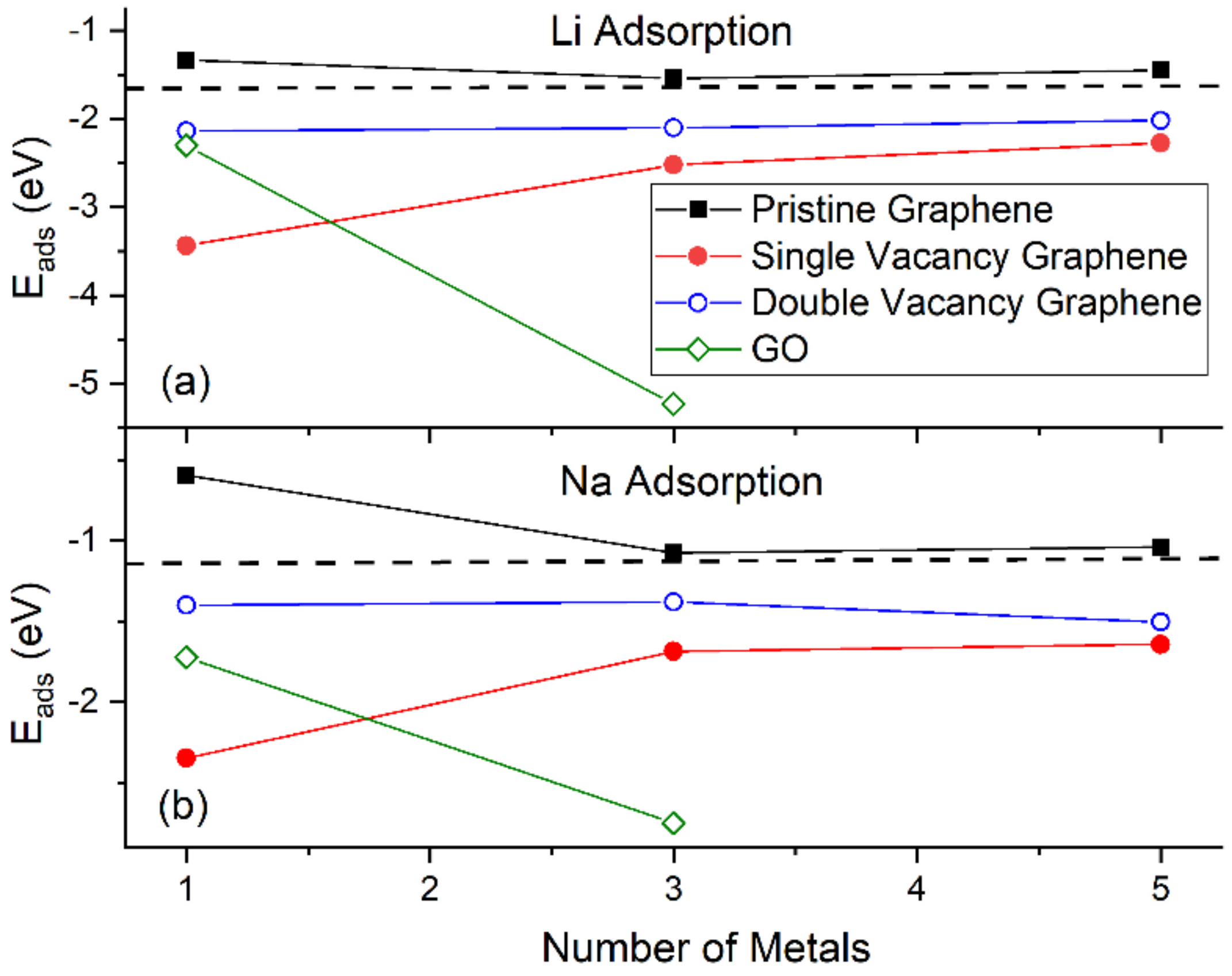
The Eads for (a) Li and (b) Na adsorptions on various supports. The horizontal dashed lines are the corresponding bulk metals Eads. Calculations include D2 correction.
Figure 4.
The Eads for (a) Li and (b) Na adsorptions on various supports. The horizontal dashed lines are the corresponding bulk metals Eads. Calculations include D2 correction.
Figure 5.
Li adsorption on pristine graphene (a–c) DOS spectra and (d–f) band structures. The red horizontal line is the Fermi energy.
Figure 5.
Li adsorption on pristine graphene (a–c) DOS spectra and (d–f) band structures. The red horizontal line is the Fermi energy.
Figure 6.
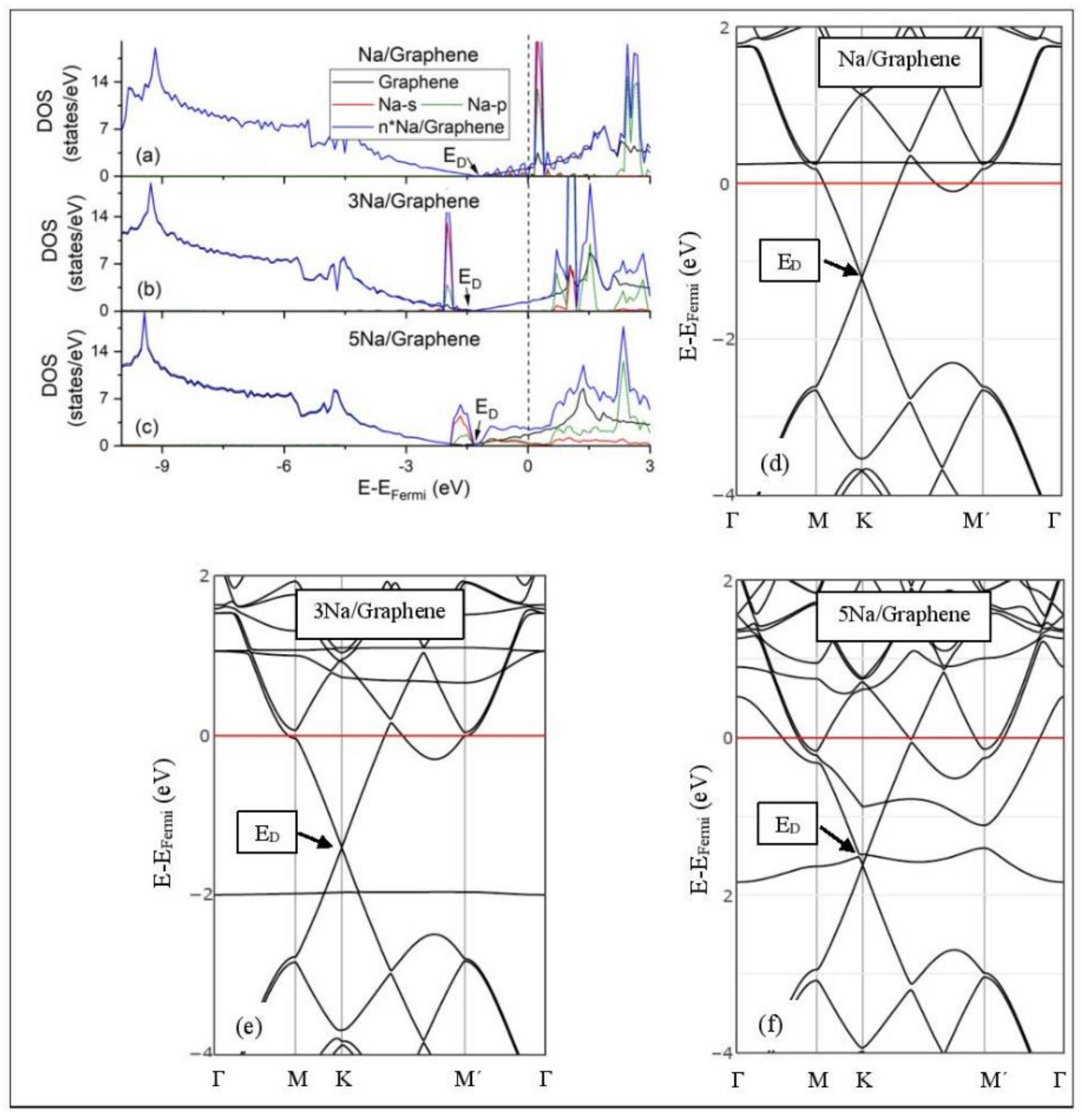
Na adsorption on pristine graphene (a–c) DOS spectra and (d–f) band structures. The red horizontal line is the Fermi energy.
Figure 6.
Na adsorption on pristine graphene (a–c) DOS spectra and (d–f) band structures. The red horizontal line is the Fermi energy.
Figure 7.
Li adsorption on defective graphene with a single vacancy per 32 C (a–c) DOS spectra and (d–f) band structures. The red horizontal line is the Fermi energy. Blue arrows show band gaps.
Figure 7.
Li adsorption on defective graphene with a single vacancy per 32 C (a–c) DOS spectra and (d–f) band structures. The red horizontal line is the Fermi energy. Blue arrows show band gaps.
Figure 8.
Li adsorption on defective graphene with double vacancies per 32 C (a–c) DOS spectra and (d–f) band structures. The red horizontal line is the Fermi energy. Blue arrows show band gaps.
Figure 8.
Li adsorption on defective graphene with double vacancies per 32 C (a–c) DOS spectra and (d–f) band structures. The red horizontal line is the Fermi energy. Blue arrows show band gaps.
Figure 9.
Na adsorption on defective graphene with single vacancy per 32 C. (a–c) DOS spectra and (d–f) band structures. The red horizontal line is the Fermi energy. Blue arrows show band gaps.
Figure 9.
Na adsorption on defective graphene with single vacancy per 32 C. (a–c) DOS spectra and (d–f) band structures. The red horizontal line is the Fermi energy. Blue arrows show band gaps.
Figure 10.
Na adsorption on defective graphene with double vacancies per 32 C (a–c) DOS spectra and (d–f) band structures. The red horizontal line is the Fermi energy. Blue arrows show band gaps.
Figure 10.
Na adsorption on defective graphene with double vacancies per 32 C (a–c) DOS spectra and (d–f) band structures. The red horizontal line is the Fermi energy. Blue arrows show band gaps.
Figure 11.
DOS spectra and band structures for adsorption on GO (a–d) Li and (e–h) Na. The red horizontal line is the Fermi energy. Blue arrows show band gaps close to the Fermi energy.
Figure 11.
DOS spectra and band structures for adsorption on GO (a–d) Li and (e–h) Na. The red horizontal line is the Fermi energy. Blue arrows show band gaps close to the Fermi energy.
Figure 12.
(a) Contour plots for Li/graphene electron density . (b) The negative of its Laplacian , which reveals saddle points (3, -1). Colors as follows: Red: High ; Blue: Low .
Figure 12.
(a) Contour plots for Li/graphene electron density . (b) The negative of its Laplacian , which reveals saddle points (3, -1). Colors as follows: Red: High ; Blue: Low .
Figure 13.
QTAIM parameters vs. metal–C distance for Li and Na adsorbed on graphene and GO. (a) , (b) , and (c) (H/ at metal–C bond critical points (cp).
Figure 13.
QTAIM parameters vs. metal–C distance for Li and Na adsorbed on graphene and GO. (a) , (b) , and (c) (H/ at metal–C bond critical points (cp).
Figure 14.
Electron localization isosurfaces for Li5 adsorbed on pristine graphene at ELF values. (a) 0.5 and (b) 0.94. Colors are as follows: C(Li) blue, C(C) red, V(Ci,Cj) green, and V(Li) and V(Li,Li) cyan. Calculations include D2 correction.
Figure 14.
Electron localization isosurfaces for Li5 adsorbed on pristine graphene at ELF values. (a) 0.5 and (b) 0.94. Colors are as follows: C(Li) blue, C(C) red, V(Ci,Cj) green, and V(Li) and V(Li,Li) cyan. Calculations include D2 correction.
Figure 15.
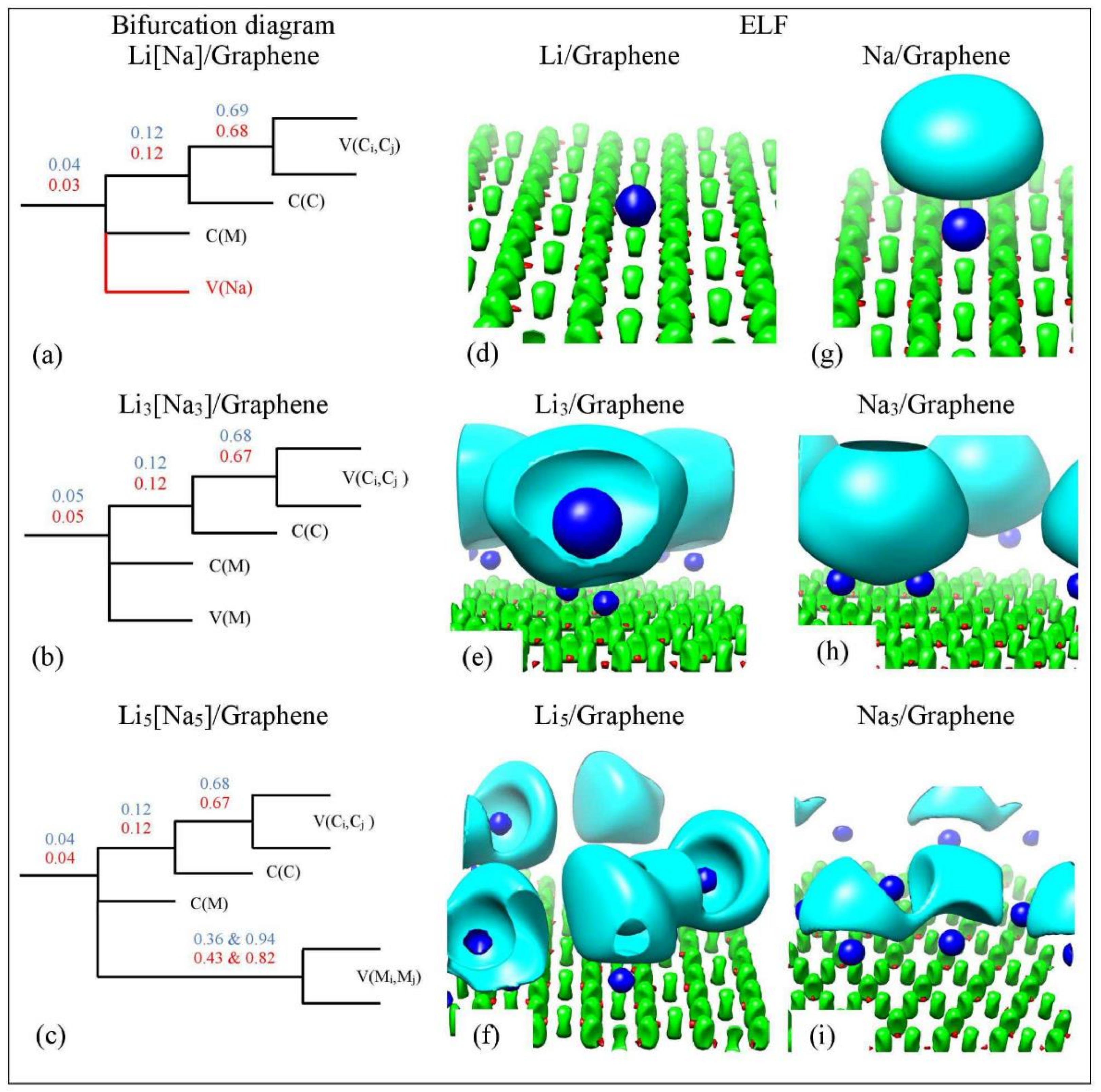
(a–c) Bifurcation diagrams for Lin and Nan n = 1, 3, 5 adsorbed on pristine graphene. Colors are as follows: blue and red refer to Li and Na adsorption, respectively and black refers to both metals. (d–i) corresponding ELF isosurfaces at ELF = 0.75. Colors are as follows: C(M) blue, C(C) red, V(Ci,Cj) green, and V(M) and V(M,M) cyan, M = Li, Na. Calculations include D2 correction.
Figure 15.
(a–c) Bifurcation diagrams for Lin and Nan n = 1, 3, 5 adsorbed on pristine graphene. Colors are as follows: blue and red refer to Li and Na adsorption, respectively and black refers to both metals. (d–i) corresponding ELF isosurfaces at ELF = 0.75. Colors are as follows: C(M) blue, C(C) red, V(Ci,Cj) green, and V(M) and V(M,M) cyan, M = Li, Na. Calculations include D2 correction.
Figure 16.
(a–c) Bifurcation diagrams for Lin and Nan n = 1, 3, 5 adsorbed on single vacancy defective graphene. Colors are as follows: blue and red refer to Li and Na adsorption, respectively, and black refers to both metals. (d–i) Corresponding ELF isosurfaces at ELF = 0.75. Colors are as follows: C(M) blue, C(C) red, V(Ci,Cj) green, and V(M) and V(M,M) cyan, M = Li, Na. M* is the metal atom close to the defect. Calculations include D2 correction.
Table 1.
Calculated Eads for Li and Na adsorbed on graphene compared with past work. Values in parentheses include D2 correction. Unless otherwise stated, the graphene support contains 32 atoms per unit cell (4 4 supercell).
Table 1.
Calculated Eads for Li and Na adsorbed on graphene compared with past work. Values in parentheses include D2 correction. Unless otherwise stated, the graphene support contains 32 atoms per unit cell (4 4 supercell).
| System | Vacancies | Current Work | Past work |
|---|
| Eads (eV) | Method |
|---|
| Li /Graphene | 0 | −1.34 (−1.33) | −1.19 [90], −1.096 [16] | PBE [91] |
| | | −1.36 [92] | LDA |
| | | −1.56 [90] | PBE+D2 [54,91] |
| | | −1.23 [90] | PBE+D3 [91,93] |
| | | −1.05 [90] | PBE+vdW-DF2 [91] |
| 1 | (−3.44) | −2.65 [94] | PBE [91] |
| | | −2.94 [94] | PBE+D2 [54,91] |
| | | −2.72 [94] | PBE+D3 [91,93] |
| | | −2.59 [94] | PBE+vdW-DF2 [91,95] |
| Na /Graphene | 0 | −0.59 (−0.59) | −0.55 [90], −0.462 [16] | PBE [91] |
| | | −0.72 [92] a | LDA |
| | | −0.93 [90] | PBE+D2 [54,91] |
| | | −0.64 [90] | PBE+D3 [91,93] |
| | | −0.49 [90] | PBE+vdW-DF2 [91,95] |
| | | −0.88 [37] | PBE+D2 [91] |
| 1 | (−2.35) | −1.88 [94] | PBE [91] |
| | | −2.20 [94] | PBE+D2 [54,91] |
| | | −2.00 [94] | PBE+D3 [91,93] |
| | | −1.74 [94] | PBE+vdW-DF2 [91,95] |
Table 2.
Li and Na Hirshfeld and Mulliken electronic charges (average values per metal) and metal–C COOP for the smaller metal–C distances, for Li and Na absorbed on graphene and GO. Values in parentheses include D2 correction.
Table 2.
Li and Na Hirshfeld and Mulliken electronic charges (average values per metal) and metal–C COOP for the smaller metal–C distances, for Li and Na absorbed on graphene and GO. Values in parentheses include D2 correction.
| Metals | Support | Vacancies | Metal charge (e) | Metal–C COOP a |
|---|
| Hirshfeld | Mulliken |
|---|
| Li | Graphene | 0 | 2.27 (2.27) | 2.66 (2.64) | 0.041 (0.040) |
| | 1 | (2.37) | (2.73) | (0.138) 3 |
| | 2 | (2.31) | (2.67) | (0.039) 6 |
| GO | 0 | 2.13 (2.14) | 2.43 (2.45) | 0.085 (0.082) 1 |
| Li3 | Graphene | 0 | 2.98 (2.98) | 2.97 (2.97) | 0.024 (0.024) |
| | 1 | (2.64) | (2.84) | (0.036) 6 |
| | 2 | (2.76) | (2.84) | (0.006) 4 |
| GO | 0 | 2.12 (2.13) | 2.42 (2.43) | 0.088 (0.090) 1 |
| Li5 | Graphene | 0 | 3.01 (3.02) | 2.99 (2.99) | 0.015 (0.022) |
| | 1 | (2.81) | (2.91) | (0.029) 6 |
| | 2 | (2.84) | (2.43) | (0.036) 6 |
| Na | Graphene | 0 | 10.53 (10.53) | 10.81 (10.58) | 0.043 (0.042) |
| | 1 | (10.32) | (10.76) | (0.116) 3 |
| | 2 | (10.21) | (10.68) | (0.043) 6 |
| GO | 0 | 10.13 (10.13) | 10.53 (10.54) | 0.051(0.050) 1 |
| Na3 | Graphene | 0 | 10.85 (10.85) | 10.97 (10.98) | 0.039 (0.039) |
| | 1 | (10.72) | (10.97) | (0.039) 6 |
| | 2 | (10.85) | (10.97) | (0.035) 6 |
| GO | 0 | 10.72 (10.52) | 10.84 (10.64) | 0.018 (0.032) |
| Na5 | Graphene | 0 | 10.95 (10.95) | 11.03 (11.04) | 0.031 (0.037) 6 |
| | 1 | (10.85) | (11.01) | (0.039) 6 |
| | 2 | (10.86) | (11.00) | (0.035) 6 |
Table 3.
QTAIM parameters , , (H/, and (G/ at the Li-C bond critical points for the shortest Li-C distances, for Li adsorbed on graphene, with and without vacancies, and GO. For adsorption on GO, these properties are also calculated at the Li-O bond critical point. Values in parentheses include D2 correction.
| Metals | Support | Vacancies | Distances (Å) | QTAIM properties (a.u.) |
|---|
| Li-C [Li-O] | | | | |
|---|
| Li | Graphene | 0 | 2.16 | 0.025 | 0.133 | 0.095 | 1.224 |
| | | (2.22) | (0.023) | (0.117) | (0.101) | (1.192) |
| | 1 | (1.98) | (0.044) | (0.197) | (< 0.01) | (1.111) |
| | 2 | (2.12) | (0.026) | (0.132) | (0.094) | (1.185) |
| GO | 0 | 2.33 | 0.017 | 0.079 | 0.127 | 1.020 |
| | | (2.26) | (0.021) | (0.093) | (0.107) | (1.000) |
| | | [(1.84)] | [(0.039)] | [(0.276)] | [(0.136)] | [(1.569)] |
| Li3 | Graphene | 0 | 2.281 | 0.0221 | 0.1361 | 0.1881 | 1.3251 |
| | | (2.30) | (0.018) | (0.093) | (0.142) | (1.147) |
| | 1 | (2.14) | (0.024) | (0.131) | (0.118) | (1.228) |
| | 2 | (2.12) | (0.025) | (0.128) | (0.099) | (1.162) |
| GO | 0 | 2.362 | 0.016 | 0.078 | 0.157 | 1.057 |
| | | (2.30) | (0.018) | (0.089) | (0.143) | (1.068) |
| | | [(1.82)] | [(0.042)] | [(0.294)] | [(0.186)] | [(1.565)] |
| Li5 | Graphene | 0 | 2.24 | 0.018 | 0.092 | 0.143 | 1.131 |
| | | (2.28) | (0.018) | (0.095) | (0.153) | (1.155) |
| | 1 | (1.99) | (0.043) | (0.188) | (< 0.01) | (1.098) |
| | 2 | (2.10) | (0.030) | (0.153) | (0.057) | (1.209) |
Table 4.
QTAIM parameters , , (H/, and (G/ at the Na-C bond critical points for the shortest Na-C distances, for Na adsorbed on graphene, with and without vacancies, and GO. For adsorption on GO, these properties are also calculated at the Li-O bond critical point. Values in parentheses include D2 correction.
| Metals | Support | Vacancies | Distances (Å) | QTAIM properties (a.u.) |
|---|
| Na-C[Na-O] | | | | |
|---|
| Na | Graphene | 0 | 2.62 | 0.015 | 0.075 | 0.147 | 1.105 |
| | | (2.64) | (0.015) | (0.073) | (0.149) | (1.098) |
| | 1 | (2.47) | (0.020) | (0.092) | (0.106) | (1.054) |
| | 2 | (2.49) | (0.020) | (0.096) | (0.108) | (1.108) |
| GO | 0 | 2.54 | 0.019 | 0.087 | 0.116 | 1.048 |
| | | (2.50) | (0.019) | (0.092) | (0.120) | (1.074) |
| | | [(2.37)] | [(0.019)] | [(0.162)] | [(0.237)] | [(1.321)] |
| Na3 | Graphene | 0 | 2.50 | 0.018 | 0.088 | 0.142 | 1.093 |
| | | (2.59) | (0.016) | (0.078) | (0.151) | (1.085) |
| | 1 | (2.40) | (0.029) | (0.127) | (0.047) | (1.031) |
| | 2 | (2.63) | (0.014) | (0.072) | (0.165) | (1.083) |
| GO | 0 | 2.87 | 0.009 | 0.043 | 0.277 | 1.005 |
| | | (2.60) | (0.016) | (0.077) | (0.155) | (1.048) |
| | | [(2.27)] | [(0.023)] | [(0.152)] | [(0.237)] | [(1.426)] |
| Na5 | Graphene | 0 | 2.75 | 0.012 | 0.059 | 0.189 | 1.027 |
| | | (2.62) | (0.014) | (0.070) | (0.179) | (1.067) |
| | 1 | (2.40) | (0.029) | (0.126) | (0.048) | (1.035) |
| | 2 | (2.51) | (0.020) | (0.090) | (0.110) | (1.001) |
Table 5.
QTAIM parameters , (H/, (G/, and and ELF at all available Li-Li bond critical points, for Li adsorbed on graphene, with and without vacancies, and GO. Here, Values in parentheses include D2 correction.
Table 5.
QTAIM parameters , (H/, (G/, and and ELF at all available Li-Li bond critical points, for Li adsorbed on graphene, with and without vacancies, and GO. Here, Values in parentheses include D2 correction.
| System | Vacancies | Li-Li (Å) | QTAIM properties (a.u.) | ELF |
|---|
| | | | |
|---|
| Li3/Graphene | 0 | 2.92 | 0.0131 | −0.159 | 0.233 | 3.37 | 0.31 |
| | 2.92 | 0.0131 | −0.158 | 0.234 | 3.28 | 0.31 |
| | (2.85) | (0.014)1 | (−0.166) | (0.243) | (3.25) | (0.31) |
| | (2.85) | (0.014)1 | (−0.165) | (0.243) | (3.21) | (0.31) |
| Li5/Graphene | 0 | 2.73 | 0.0112 | −0.174 | 0.093 | −3.09 | 0.69 |
| | 2.97 | 0.0111 | −0.150 | 0.228 | 3.20 | 0.28 |
| | 3.04 | 0.0131 | −0.153 | 0.249 | 2.55 | 0.30 |
| | (2.77) | (<0.01)2 | (−0.148) | (0.044) | (−2.40) | (0.89) |
| | (2.91) | (0.010)2 | (−0.170) | (0.164) | (−40.60) | (0.39) |
| | (2.92) | (0.012)1 | (−0.163) | (0.211) | (5.27) | (0.34) |
| 1 | (2.70) | (<0.01)1 | (−0.115) | (0.227) | (2.24) | (0.22) |
| | (2.84) | (0.011)1 | (−0.159) | (0.215) | (4.24) | (0.32) |
| | (3.18) | (<0.01)1 | (−0.128) | (0.246) | (2.13) | (0.21) |
| 2 | (2.87) | (0.010)1 | (−0.152) | (0.214) | (4.07) | (0.29) |
| | (3.37) | (<0.01)1 | (−0.115) | (0.251) | (1.84) | (0.18) |
| | (3.49) | (<0.01)1 | (−0.087) | (0.233) | (1.71) | (0.11) |
Table 6.
QTAIM parameters , (H/, (G/, and and ELF at all available Na-Na bond critical points, for Na adsorbed on graphene, with and without vacancies, and GO. Here, Values in parentheses include D2 correction.
Table 6.
QTAIM parameters , (H/, (G/, and and ELF at all available Na-Na bond critical points, for Na adsorbed on graphene, with and without vacancies, and GO. Here, Values in parentheses include D2 correction.
| System | Vacancies | Na-Na (Å) | QTAIM properties (a.u) | ELF |
|---|
| | | | |
|---|
| Na3/Graphene | 0 | 3.35 | 0.091 | −0.103 | 0.186 | 3.02 | 0.31 |
| | 3.37 | 0.091 | −0.096 | 0.197 | 2.50 | 0.28 |
| | (3.23) | (0.10)1 | (−0.109) | (0.205) | (2.60) | (0.30) |
| | (3.24) | (0.10)1 | (−0.108) | (0.207) | (2.51) | (0.29) |
| 1 | (3.82)3 | (0.04)2 | (−0.124) | (0.054) | (−3.59) | (0.65) |
| 2 | (3.35) | (0.08)1 | (−0.099) | (0.190) | (2.75) | (0.28) |
| | (3.38) | (0.08)1 | (−0.093) | (0.198) | (2.38) | (0.26) |
| Na3/GO | 0 | 3.34 | 0.091 | −0.097 | 0.184 | 2.84 | 0.30 |
| | 3.43 | 0.081 | −0.088 | 0.195 | 2.33 | 0.26 |
| | (3.19) | 0.052 | (−0.151) | (0.137) | (−17.51) | (0.28) |
| Na5/Graphene | 0 | 3.66 | 0.062 | −0.114 | 0.061 | -4.71 | 0.71 |
| | 4.10 | 0.061 | −0.104 | 0.114 | 26.06 | 0.43 |
| | (3.54) | 0.072 | (−0.121) | (0.029) | (−2.71) | (0.93) |
| | (4.05) | (0.07)1 | (−0.110) | (0.141) | (8.04) | (0.34) |
| 1 | (3.55) | (0.06)1 | (−0.113) | (0.115) | (201.62) | (0.41) |
| | (3.63) | (0.06)1 | (−0.089) | (0.151) | (4.017) | (0.28) |
| 2 | (3.34) | (0.07)1 | (−0.084) | (0.220) | (1.84) | (0.20) |
| | (3.41) | (0.07)1 | (−0.090) | (0.182) | (2.70) | (0.26) |

 ,
, 


