Prediction of Chromatographic Elution Order of Analytical Mixtures Based on Quantitative Structure-Retention Relationships and Multi-Objective Optimization


Abstract
:1. Introduction
2. Results and Discussion
3. Materials and Methods
3.1. Chromatographic Measurements
3.2. QSRR Model Development
3.3. QSRR Model Validation
3.4. Elution Order Prediction
3.5. Multi-Objective Optimization (MOO)
3.6. Objective Functions for MOO
3.7. Selection of an Optimal MOO Solution
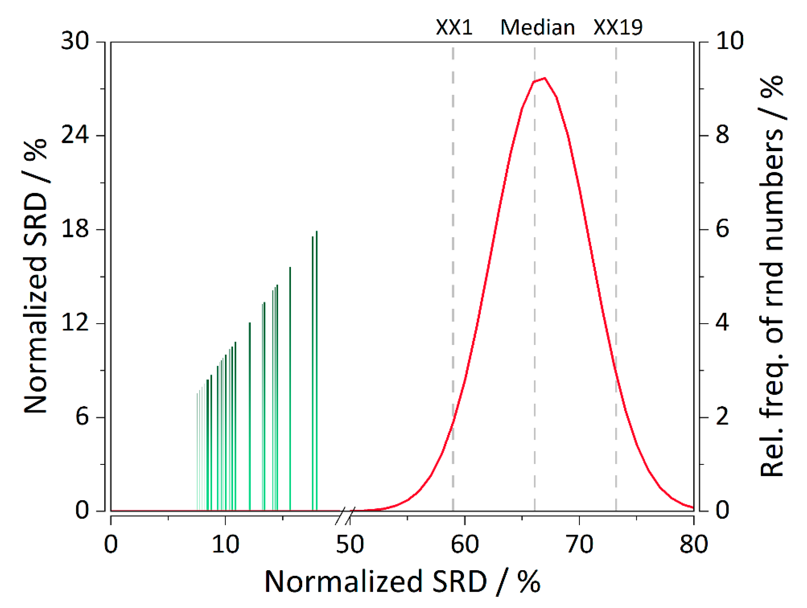
3.8. Sum of Ranking Differences
3.9. Software Development
4. Conclusions
5. Patents
Supplementary Materials
Author Contributions
Funding
Acknowledgments
Conflicts of Interest
References
- Žuvela, P.; Skoczylas, M.; Liu, J.J.; Baczek, T.; Kaliszan, R.; Wong, M.W.; Buszewski, B. Column Characterization and Selection Systems in Reversed-Phase High-Performance Liquid Chromatography. Chem. Rev. 2019, 119, 3674–3729. [Google Scholar] [CrossRef]
- Kaliszan, R. QSRR: Quantitative Structure-(Chromatographic) Retention Relationships. Chem. Rev. 2007, 107, 3212–3246. [Google Scholar] [CrossRef]
- Vorslova, S.; Golushko, J.; Galushko, S.; Viksna, A. Prediction of Reversed-Phase Liquid Chromatography Retention Parameters for Phenylisothiocyanate Derivatives of Amino Acids. Latv. J. Chem. 2014, 52, 61–70. [Google Scholar] [CrossRef]
- Shinoda, K.; Sugimoto, M.; Yachie, N.; Sugiyama, N.; Masuda, T.; Robert, M.; Soga, T.; Tomita, M. Prediction of Liquid Chromatographic Retention Times of Peptides Generated by Protease Digestion of the Escherichia coli Proteome Using Artificial Neural Networks. J. Proteome Res. 2006, 5, 3312–3317. [Google Scholar] [CrossRef]
- Bach, E.; Szedmak, S.; Brouard, C.; Böcker, S.; Rousu, J. Liquid-chromatography retention order prediction for metabolite identification. Bioinformatics 2018, 34, i875–i883. [Google Scholar] [CrossRef]
- Liu, J.J.; Alipuly, A.; Baczek, T.; Wong, M.W.; Žuvela, P.; Liu, W. Quantitative Structure-Retention Relationships with Non-Linear Programming for Prediction of Chromatographic Elution Order. Int. J. Mol. Sci. 2019, 20, 3443. [Google Scholar] [CrossRef] [Green Version]
- Galushko, S.; Kamenchuk, A.; Pit, G. Calculation of retention in reversed-phase liquid chromatography. J. Chromatogr. A 1994, 660, 47–59. [Google Scholar] [CrossRef]
- Petritis, K.; Kangas, L.J.; Yan, B.; Monroe, M.E.; Strittmatter, E.F.; Qian, W.-J.; Adkins, J.N.; Moore, R.J.; Xu, Y.; Lipton, M.S.; et al. Improved Peptide Elution Time Prediction for Reversed-Phase Liquid Chromatography-MS by Incorporating Peptide Sequence Information. Anal. Chem. 2006, 78, 5026–5039. [Google Scholar] [CrossRef] [Green Version]
- Petritis, K.; Kangas, L.J.; Ferguson, P.L.; Anderson, G.A.; Paša-Tolić, L.; Lipton, M.S.; Auberry, K.J.; Strittmatter, E.F.; Shen, Y.; Zhao, R.; et al. Use of Artificial Neural Networks for the Accurate Prediction of Peptide Liquid Chromatography Elution Times in Proteome Analyses. Anal. Chem. 2003, 75, 1039–1048. [Google Scholar] [CrossRef]
- Wu, Y. Statistical Learning Theory. Technometrics 1999, 41, 377–378. [Google Scholar] [CrossRef]
- Bellman, R. On the Theory of Dynamic Programming. Proc. Natl. Acad. Sci. USA 1952, 38, 716–719. [Google Scholar] [CrossRef] [PubMed] [Green Version]
- Kaliszan, R.; Van Straten, M.A.; Markuszewski, M.; Cramers, C.A.; Claessens, H.A. Molecular mechanism of retention in reversed-phase high-performance liquid chromatography and classification of modern stationary phases by using quantitative structure-retention relationships. J. Chromatogr. A 1999, 855, 455–486. [Google Scholar] [CrossRef]
- Baczek, T.; Wiczling, P.; Marszałł, M.; Heyden, Y.V.; Kaliszan, R. Prediction of Peptide Retention at Different HPLC Conditions from Multiple Linear Regression Models. J. Proteome Res. 2005, 4, 555–563. [Google Scholar] [CrossRef]
- Buszewski, B.; Žuvela, P.; Sagandykova, G.N.; Walczak-Skierska, J.; Pomastowski, P.; David, J.; Wong, M.W. Mechanistic Chromatographic Column Characterization for the Analysis of Flavonoids Using Quantitative Structure-Retention Relationships Based on Density Functional Theory. Int. J. Mol. Sci. 2020, 21, 2053. [Google Scholar] [CrossRef] [Green Version]
- Žuvela, P.; Liu, J.J.; Macur, K.; Baczek, T. Molecular Descriptor Subset Selection in Theoretical Peptide Quantitative Structure–Retention Relationship Model Development Using Nature-Inspired Optimization Algorithms. Anal. Chem. 2015, 87, 9876–9883. [Google Scholar] [CrossRef]
- Wolpert, D.; Macready, W. No free lunch theorems for optimization. IEEE Trans. Evol. Comput. 1997, 1, 67–82. [Google Scholar] [CrossRef] [Green Version]
- Baczek, T.; Kaliszan, R.; Novotná, K.; Jandera, P. Comparative characteristics of HPLC columns based on quantitative structure-retention relationships (QSRR) and hydrophobic-subtraction model. J. Chromatogr. A 2005, 1075, 109–115. [Google Scholar] [CrossRef]
- Kaliszan, R.; Baczek, T.; Bucinski, A.; Buszewski, B.; Sztupecka, M.; Baczek, T. Prediction of gradient retention from the linear solvent strength (LSS) model, quantitative structure-retention relationships (QSRR), and artificial neural networks (ANN). J. Sep. Sci. 2003, 26, 271–282. [Google Scholar] [CrossRef]
- Yu, H.; He, X.; Li, S.; Truhlar, D.G. MN15: A Kohn–Sham global-hybrid exchange–correlation density functional with broad accuracy for multi-reference and single-reference systems and noncovalent interactions† †Electronic supplementary information (ESI) available: Mean unsigned errors of Database 2015B for 84 functionals and geometries of databases ABDE13, S6x6, SBG31, and EE69. Chem. Sci. 2016, 7, 5032–5051. [Google Scholar] [CrossRef] [Green Version]
- Rassolov, V.A.; Ratner, M.A.; Pople, J.A.; Redfern, P.C.; Curtiss, L.A. 6-31G* basis set for third-row atoms. J. Comput. Chem. 2001, 22, 976–984. [Google Scholar] [CrossRef]
- Marenich, A.V.; Cramer, C.J.; Truhlar, D.G. Universal Solvation Model Based on Solute Electron Density and on a Continuum Model of the Solvent Defined by the Bulk Dielectric Constant and Atomic Surface Tensions. J. Phys. Chem. B 2009, 113, 6378–6396. [Google Scholar] [CrossRef]
- Kaliszan, R.; Baczek, T.; Cimochowska, A.; Juszczyk, P.; Wi?niewska, K.; Grzonka, Z.; Baczek, T.; Wiśniewska, K. Prediction of high-performance liquid chromatography retention of peptides with the use of quantitative structure-retention relationships. Proteomes 2005, 5, 409–415. [Google Scholar] [CrossRef]
- Bodzioch, K.; Durand, A.; Kaliszan, R.; Baczek, T.; Heyden, Y.V. Advanced QSRR modeling of peptides behavior in RPLC. Talanta 2010, 81, 1711–1718. [Google Scholar] [CrossRef]
- Bodzioch, K.; Dejaegher, B.; Baczek, T.; Kaliszan, R.; Heyden, Y.V. Evaluation of a generalized use of the log Sum(k+1)AAdescriptor in a QSRR model to predict peptide retention on RPLC systems. J. Sep. Sci. 2009, 32, 2075–2083. [Google Scholar] [CrossRef]
- Efroymson, M.A. Multiple Regression Analysis. In Mathematical Methods for Digital Computers; WILEY-VCH Verlag: New York, NY, USA, 1960. [Google Scholar]
- Kennard, R.W.; Stone, L.A. Computer Aided Design of Experiments. Technometrics 1969, 11, 137–148. [Google Scholar] [CrossRef]
- Žuvela, P.; Macur, K.; Liu, J.J.; Baczek, T. Exploiting non-linear relationships between retention time and molecular structure of peptides originating from proteomes and comparing three multivariate approaches. J. Pharm. Biomed. Anal. 2016, 127, 94–100. [Google Scholar] [CrossRef]
- Holland, J.H. Adaptation in Natural and Artificial Systems; MIT Press: Cambridge, MA, USA, 1992. [Google Scholar]
- Forrest, S. Genetic algorithms: Principles of natural selection applied to computation. Science 1993, 261, 872–878. [Google Scholar] [CrossRef] [Green Version]
- Wright, M.H. The interior-point revolution in optimization: History, recent developments, and lasting consequences. Bull. Am. Math. Soc. 2004, 42, 39–57. [Google Scholar] [CrossRef] [Green Version]
- Møller, M.F. A scaled conjugate gradient algorithm for fast supervised learning. Neural Netw. 1993, 6, 525–533. [Google Scholar] [CrossRef]
- Taraji, M.; Haddad, P.R.; Amos, R.I.; Talebi, M.; Szucs, R.; Dolan, J.W.; Pohl, C.A. Error measures in quantitative structure-retention relationships studies. J. Chromatogr. A 2017, 1524, 298–302. [Google Scholar] [CrossRef] [PubMed]
- Heberger, K. Sum of ranking differences compares methods or models fairly. TrAC Trends Anal. Chem. 2010, 29, 101–109. [Google Scholar] [CrossRef]
- West, C.; Khalikova, M.A.; Lesellier, E.; Héberger, K. Sum of ranking differences to rank stationary phases used in packed column supercritical fluid chromatography. J. Chromatogr. A 2015, 1409, 241–250. [Google Scholar] [CrossRef]
- Andrić, F.; Héberger, K. How to compare separation selectivity of high-performance liquid chromatographic columns properly? J. Chromatogr. A 2017, 1488, 45–56. [Google Scholar] [CrossRef] [Green Version]
- Héberger, K.; Kollár-Hunek, K. Sum of ranking differences for method discrimination and its validation: Comparison of ranks with random numbers. J. Chemom. 2011, 25, 151–158. [Google Scholar] [CrossRef]


| CS a | Column Name | Analysis Parameters b | Model | %RMSE(tR) | %RMSE(Order) | SRD/% |
|---|---|---|---|---|---|---|
| I | Supelcosil LC-18 | tG = 10 min T = 35 °C | MLR (control) | 8.57 | 59.07 | N/A |
| MLR-MOO | 9.33 | 42.04 | N/A | |||
| II | Xterra MS C18 | tG = 20 min T = 40 °C | MLR (control) | 11.50 | 25.01 | 8.12 |
| MLR-MOO | 12.07 | 18.05 | 7.58 | |||
| II | LiChrospher RP-18 | tG = 20 min T = 40 °C | MLR (control) | 13.25 | 30.28 | 7.79 |
| MLR-MOO | 13.31 | 22.23 | 8.00 | |||
| II | LiChrospher RP-18 | tG = 60 min T = 40 °C | MLR (control) | 25.60 | 34.11 | 10.04 |
| MLR-MOO | 26.84 | 20.50 | 7.71 | |||
| II | LiChrospher RP-18 | tG = 120 min T = 40 °C | MLR (control) | 42.31 | 153.00 | 14.16 |
| MLR-MOO | 47.43 | 26.82 | 9.58 | |||
| II | LiChrospher RP-18 | tG = 20 min T = 60 °C | MLR (control) | 18.45 | 36.12 | 8.45 |
| MLR-MOO | 18.58 | 31.09 | 7.91 | |||
| II | LiChrospher RP-18 | tG = 20 min T = 80 °C | MLR (control) | 18.82 | 35.25 | 8.33 |
| MLR-MOO | 18.83 | 34.10 | 8.75 | |||
| II | Licrospher CN | tG = 20 min T = 40 °C | MLR (control) | 39.28 | 195.82 | 13.20 |
| MLR-MOO | 40.85 | 31.08 | 10.37 | |||
| II | PLRP-S | tG = 20 min T = 40 °C | MLR (control) | 20.07 | 69.44 | 9.95 |
| MLR-MOO | 21.89 | 44.54 | 10.41 | |||
| II | PLRP-S | tG = 60 min T = 40 °C | MLR (control) | 37.92 | 107.94 | 13.41 |
| MLR-MOO | 39.28 | 46.84 | 9.83 | |||
| II | PLRP-S | tG = 20 min T = 60 °C | MLR (control) | 21.75 | 94.97 | 10.83 |
| MLR-MOO | 21.94 | 55.19 | 9.95 | |||
| II | PLRP-S | tG = 60 min T = 60 °C | MLR (control) | 40.11 | 321.65 | 13.24 |
| MLR-MOO | 44.91 | 47.01 | 9.54 | |||
| II | PLRP-S | tG = 20 min T = 80 °C | MLR (control) | 22.36 | 137.16 | 12.12 |
| MLR-MOO | 22.71 | 55.35 | 10.87 | |||
| II | PLRP-S | tG = 60 min T = 80 °C | MLR (control) | 42.60 | 194.56 | 14.37 |
| MLR-MOO | 45.16 | 44.38 | 9.70 | |||
| II | Discovery RP Amide C16 | tG = 20 min T = 40 °C | MLR (control) | 36.73 | 261.22 | 17.95 |
| MLR-MOO | 37.58 | 75.84 | 15.62 | |||
| II | Discovery RP Amide C16 | tG = 20 min T = 60 °C | MLR (control) | 36.37 | 219.01 | 17.62 |
| MLR-MOO | 36.98 | 70.10 | 15.66 | |||
| II | Discovery RP Amide C16 | tG = 20 min T = 80 °C | MLR (control) | 36.74 | 241.63 | 14.54 |
| MLR-MOO | 38.01 | 69.92 | 13.29 | |||
| II | Discovery HS F5 | tG = 20 min T = 40 °C | MLR (control) | 12.81 | 34.00 | 10.58 |
| MLR-MOO | 14.43 | 22.08 | 9.33 | |||
| II | Chromolith | tG = 20 min T = 40 °C | MLR (control) | 20.82 | 43.81 | 8.20 |
| MLR-MOO | 21.34 | 32.55 | 9.25 |
| # | Column Name | Length/mm | Internal Diameter (ID)/mm | Particle Size/μm | Carbon Load (C)/% | Pore Size/Å | Surface Area/m2 g |
|---|---|---|---|---|---|---|---|
| 1 | Xterra MS C18 | 150 | 4.6 | 3.5 | 15.5 | 125 | 175 |
| 2 | LiChrospher RP-18 | 250 | 4.6 | 5.0 | 21.0 | 100 | 350 |
| 3 | LiChrospher CN | 125 | 4.6 | 5.0 | 6.6 | 100 | 350 |
| 4 | Discovery HS F5-3 | 150 | 4.6 | 3.0 | 12.0 | 120 | 300 |
| 5 | Discovery RP Amide C16 | 150 | 4.6 | 5.0 | 11.0 | 180 | 200 |
| 6 | Chromolith | 100 | 4.6 | 2.0 | 18.0 | 130 | 300 |
| 7 | PLRP-S | 150 | 4.1 | 5.0 | 16.0 | 100 | 300 |
| 8 | Supelcosil LC-18 | 150 | 4.6 | 5.0 | 11.0 | 120 | 170 |
© 2020 by the authors. Licensee MDPI, Basel, Switzerland. This article is an open access article distributed under the terms and conditions of the Creative Commons Attribution (CC BY) license (http://creativecommons.org/licenses/by/4.0/).
Share and Cite
Žuvela, P.; Liu, J.J.; Wong, M.W.; Bączek, T. Prediction of Chromatographic Elution Order of Analytical Mixtures Based on Quantitative Structure-Retention Relationships and Multi-Objective Optimization. Molecules 2020, 25, 3085. https://doi.org/10.3390/molecules25133085
Žuvela P, Liu JJ, Wong MW, Bączek T. Prediction of Chromatographic Elution Order of Analytical Mixtures Based on Quantitative Structure-Retention Relationships and Multi-Objective Optimization. Molecules. 2020; 25(13):3085. https://doi.org/10.3390/molecules25133085
Chicago/Turabian StyleŽuvela, Petar, J. Jay Liu, Ming Wah Wong, and Tomasz Bączek. 2020. "Prediction of Chromatographic Elution Order of Analytical Mixtures Based on Quantitative Structure-Retention Relationships and Multi-Objective Optimization" Molecules 25, no. 13: 3085. https://doi.org/10.3390/molecules25133085
APA StyleŽuvela, P., Liu, J. J., Wong, M. W., & Bączek, T. (2020). Prediction of Chromatographic Elution Order of Analytical Mixtures Based on Quantitative Structure-Retention Relationships and Multi-Objective Optimization. Molecules, 25(13), 3085. https://doi.org/10.3390/molecules25133085