Ultraviolet Spectroscopic Detection of Nitrate and Nitrite in Seawater Simultaneously Based on Partial Least Squares

Abstract

A direct, reagent-free, ultraviolet spectroscopic method for the simultaneous determination of nitrate (NO₃⁻), nitrite (NO₂⁻), and salinity in seawater is presented. The method is based on measuring the absorption spectra of the raw seawater range of 200–300 nm, combined with partial least squares (PLS) regression for resolving the spectral overlapping of NO₃⁻, NO₂⁻, and sea salt (or salinity). The interference from chromophoric dissolved organic matter (CDOM) UV absorbance was reduced according to its exponential relationship between 275 and 295 nm. The results of the cross-validation of calibration and the prediction sets were used to select the number of factors (4 for NO₃⁻, NO₂⁻, and salinity) and to optimize the wavelength range (215–240 nm) with a 1 nm wavelength interval. The linear relationship between the predicted and the actual values of NO₃⁻, NO₂⁻, salinity, and the recovery of spiked water samples suggest that the proposed PLS model can be a valuable alternative method to the wet chemical methods. Due to its simplicity and fast response, the proposed PLS model can be used as an algorithm for building nitrate and nitrite sensors. The comparison study of PLS and a classic least squares (CLS) model shows both PLS and CLS can give satisfactory results for predicting NO₃⁻ and salinity. However, for NO₂⁻ in some samples, PLS is superior to CLS, which may be due to the interference from unknown substances not included in the CLS algorithm. The proposed method was applied to the analysis of NO₃⁻, NO₂⁻, and salinity in the Changjiang (Yangtze River) estuary water samples and the results are comparable with that determined by the colorimetric Griess assay.

1. Introduction

Nitrate (NO₃⁻) and nitrite (NO₂⁻) are the essential nutrients for marine phytoplankton growth and play a key role in many biogeochemical cycles [1,2]. NO₃⁻and NO₂⁻ concentrations in seawater are also important indicators of water quality. Due to human activities, large amounts of nutrients are discharged into natural waters, thereby destroying the ecological balance and causing the eutrophication of water bodies [3]. Therefore, accurate quantification of NO₃⁻ and NO₂⁻ is critical for understanding the dynamics of marine ecosystems. Wet chemical analyses of NO₃⁻ and NO₂⁻ in seawater (e.g., the Griess assay) have been previously reviewed in the literature [4,5,6]. These chemical methods require the addition of chemical reagents, and thus, are time-consuming, and waste is generated during measurement.

Ultraviolet (UV) spectroscopy is another well-known method for determining NO₃⁻, which is based on the strong UV absorption spectrum of NO₃⁻ [7]. It is a standard method for NO₃⁻ analysis by the American Public Health Association [8]. The advantages of this method include its simplicity and speed of data acquisition. It avoids the use of any chemical reagents. Therefore, it can easily be developed into an underwater sensor for long-term monitoring. However, this method is susceptible to interference from high concentrations of Cl⁻ and Br⁻ (or sea salt, salinity) in seawater, which have strong UV absorbance in the NO₃⁻ absorption range [9]. Previously, multi-wavelength measurement and classic least square (CLS) regression were used to separate the overlapping spectra and measure NO₃⁻ [9,10,11,12]. However, it did not take NO₂⁻ into account. Although NO₂⁻ is the least abundant of the major inorganic nitrogen ions (NH₄⁺, NO₃⁻, and NO₂⁻) [13], it can accumulate at concentrations up to 10 μM in low-oxygen estuary and coastal waters, oxygen-deficient zones, and upwelling regions [14,15,16,17,18]. In these areas, NO₂⁻ may influence the NO₃⁻ measurement considering NO₂⁻ has a similar UV absorption spectrum to that of NO₃⁻ (Figure 1). To date, there is no report on simultaneous determination of NO₃⁻ and NO₂⁻ in seawater using UV spectroscopy. Langergraber et al. (2003) and Rieger et al. (2004, 2008) used a submersible UV/VIS spectrometer combined with partial least squares (PLS) regressions to monitor NO₃⁻, NO₂⁻, and even chemical oxygen demand, in the effluent of municipal wastewater treatment plants [19,20,21]. However, this method cannot be applied to analyze NO₃⁻ and NO₂⁻ in seawater. The reason for this is that they do not eliminate the interference from sea salt and chromophoric dissolved organic matter (CDOM) in seawater.

In this study, we aimed to (1) develop a direct, reagent-free, ultraviolet spectroscopic method to determine NO₃⁻, NO₂⁻, and salinity simultaneously based on the PLS model: (2) select an appropriate number of factors and optimal wavelength range for the PLS model; (3) evaluate the performance of the proposed method; (4) compare the results of the PLS and CLS models; (5) apply the proposed method to estuarine water samples.

2. Theory

2.1. PLS Regressions

PLS is a kind of multivariate calibration method based on factor analysis. It is a combination of principal component analysis, multiple linear regression analysis, and canonical correlation analysis. The theoretical basis for PLS regression can be found in several references [22,23,24,25,26]. PLS establishes a quantitative relationship (Equations (1) and (2)) between an n × m matrix (X) of independent variables (absorbance at each wavelength, in this case) and an n × k matrix (Y) of the predicted values of the variables (NO₃⁻, NO₂⁻, and salinity, in this case). The PLS model can be written as follows

X = TP^T + E

(1)

Y = UQ^T + F

(2)

where P and Q are the loading matrices of X and Y, which give information about weights for each predictor in X when calculating latent variables (factors); E and F are the matrices of X and Y residuals (both with the same dimensions as the original absorbance and concentration matrices, respectively); T and U represent the score matrix for X and Y, which can summarize X and predict Y with small errors in E and F. The decompositions of X and Y are made to maximize the covariance between T and U. The PLS model is built using a calibration or training set of samples that have known property values. Following the establishment of a satisfactory model, the property values in a prediction set of samples can be predicted. Here, the experimental spectra (matrix X) of single and mix standards, with known concentrations NO₃⁻, NO₂⁻, and salinity (matrix Y), were used as the calibration set.

PLS calibration of a multi-component system can be performed in two different ways, PLS1 and PLS2. In PLS1, a separate set of scores and loading vectors is tuned and calculated for each variable (NO₃⁻, NO₂⁻, and salinity). In PLS2, several variables (NO₃⁻, NO₂⁻, and salinity) are fitted simultaneously, and there is one common set of factors for NO₃⁻, NO₂⁻, and salinity [25,27]. Therefore, PLS1 should give more accurate predictions than PLS2, especially when one of the variables is influenced by a number of factors different to other variables in the mixture [26,28,29]. However, PLS2 can simplify the procedure and allows for simultaneous graphical inspection. Thus, PLS2 is faster to use than PLS1. However, it should be noted that PLS2 usually performs equally well or worse than PLS1 if there is a weak or no correlation between response variables [30,31]. In the present study, the results from PLS1 and PLS2 models are compared.

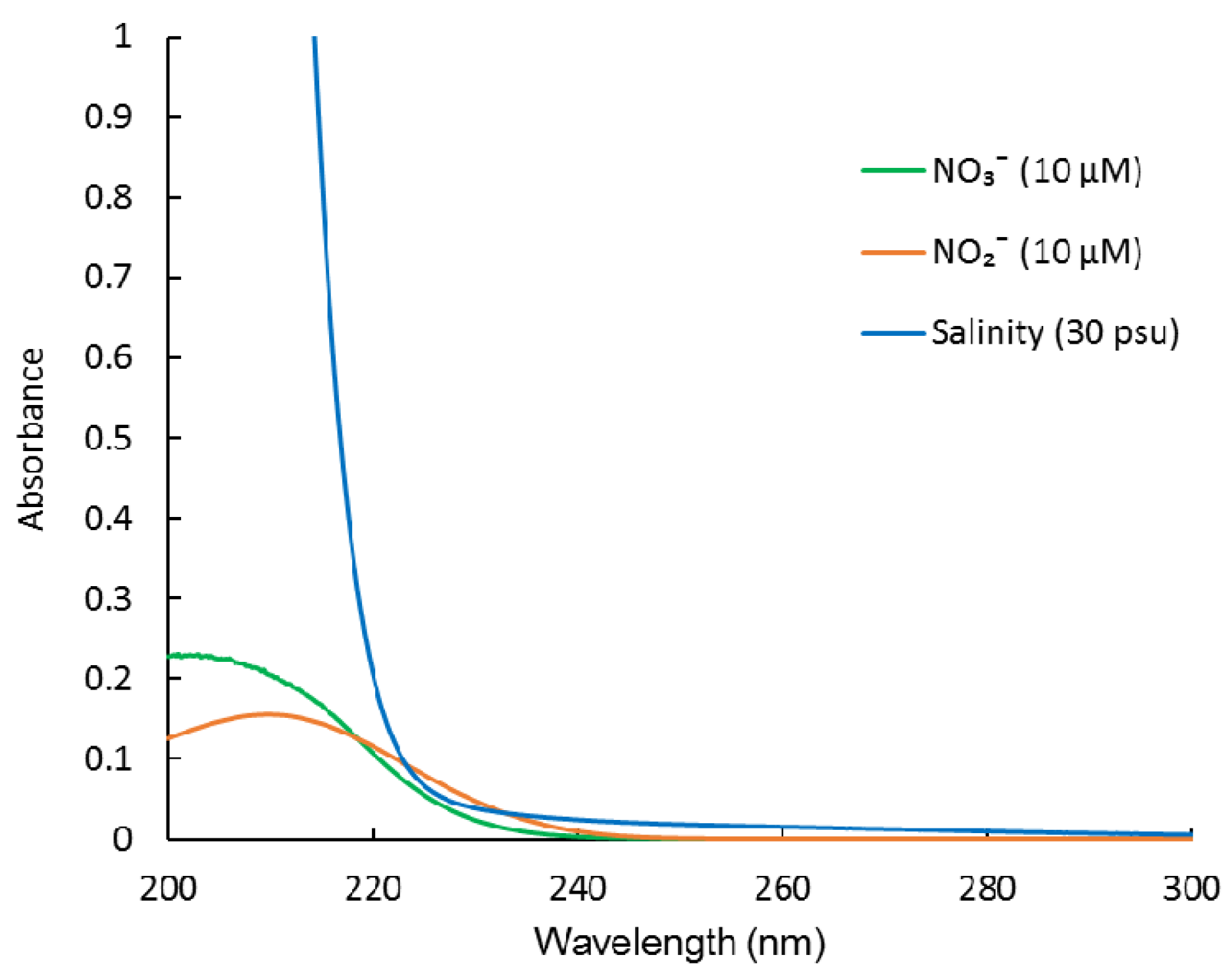
2.2. Interference from CDOM

CDOM comprises a significant fraction of the DOM pool in natural waters (~10–90%) [32]. It has strong absorption in the UV range [33,34]. Thus, the interference with NO₃⁻ and NO₂⁻ from CDOM is of particular concern. CDOM is a mixture of many organic compounds that differ spatially and temporally due to their origin. The spectral shapes of CDOM vary with the compositions of CDOM. It is difficult to link optical absorbance directly to CDOM concentrations or compositions [35,36]. Therefore, CDOM cannot be added to the predictor variable list for the model building. Many previous studies have suggested that the UV absorption spectrum of CDOM in seawater fits an exponential function with wavelengths [36,37,38,39], which can be given in Equation (3)

$${\mathrm{A}}_{\mathrm{CDOM}}\left(\mathsf{\lambda }\right)={\mathrm{A}}_{\mathrm{CDOM}}\left({\mathsf{\lambda }}_0\right){\mathrm{e}}^{\mathrm{S}\left({\mathsf{\lambda }}_0-\mathsf{\lambda }\right)}+\mathrm{k}$$

(3)

where λ is the wavelength (nm), λ₀ is a reference wavelength (nm); A_CDOM($\mathsf{\lambda }$) and A_CDOM(${\mathsf{\lambda }}_0$) are the CDOM absorbance at the wavelength of λ and λ₀; k is a background constant (m⁻¹), which accounts for light scattering in the cuvette and drift of the instrument. S is the spectral slope (nm⁻¹) that describes the approximate exponential rate of decrease in absorption with increasing wavelengths. In Equation (3), S and a are used to define differences among different samples. Usually, S is calculated over a broad wavelength range (e.g., 275–295, 350–400, and 300–600 nm) [36,38,39]. Several previous studies used a quadratic function [9,40] or linear function [41,42] to fit, approximately, the CDOM spectra. Given the comparatively high concentrations of CDOM in estuarine and coastal waters, in this study, we used an exponential function to fit the absorption spectrum of CDOM between 275 to 295 nm. The wavelength 300 nm was chosen as the reference wavelength (λ₀). Then this function was applied to the wavelength from 200 to 240 nm. Thus, the CDOM absorbance can be subtracted from the raw spectra in the developed PLS model.

2.3. CLS Regression

CLS is the simplest and most widely used technique for solving overdetermined systems. In its most important application—data fitting—it finds a hyperplane through a set of data points while minimizing the sum of squared errors [43,44]. For comparison with PLS, we also used CLS regression to fit the absorbance spectra of seawater samples and obtain NO₃⁻ and NO₂⁻ concentrations according to Equation (4)

$${\mathrm{A}}_{\mathsf{\lambda }}=\mathrm{b}\left({\mathsf{\epsilon }}_{{\mathrm{NO}}_3{}^{-}}\times {\mathrm{C}}_{{\mathrm{NO}}_3{}^{-}}+{\mathsf{\epsilon }}_{{\mathrm{NO}}_2{}^{-}}\times {\mathrm{C}}_{{\mathrm{NO}}_2{}^{-}}+{\mathsf{\epsilon }}_{\mathrm{salinity}}\times \mathrm{salinity}\right)+{\mathrm{A}}_{\mathrm{CDOM}}$$

(4)

where b is the pathlength (cm) of the optical cell, ε is the absorption coefficient of the subscripted species (L mol⁻¹ m⁻¹ for NO₃⁻ and NO₂⁻, PSU⁻¹ m⁻¹ for salinity), C is the concentration of the subscripted species. Each ε value can be obtained by measuring the absorption in standard solutions of each chemical species. The concentrations of NO₃⁻, NO₂⁻, salinity, and all the CDOM coefficients (Equation (4)), were fitted together.

3. Experimental

3.1. Reagents

All chemicals were of analytical reagent grade and supplied by the Sigma-Aldrich Company (Shanghai, China). The standard solutions of NO₃⁻ and NO₂⁻ were freshly prepared from NaNO₃, NaNO₂, and deionized water (Milli-Q water, 18.2 MΩ) before use.

3.2. Apparatus and Software

A UV-Vis spectrophotometer (Specord plus 210, Analytik Jena AG, Germany) was used to collect absorbance data from 200 to 300 nm. Due to the comparatively low concentrations and absorbance of NO₂⁻, all the samples were measured in a 3.0 cm quartz cuvette. Milli-Q water was used as the reference. The spectral resolution was set as 1 nm. A higher resolution (e.g., 0.2–0.8 nm) yields similar results. All data-processing scripts, including PLS1, PLS2 (see the Supplementary Materials), and CLS regressions, were written in MATLAB for Windows (Mathworks, version 2019b).

3.3. Model Validation

The evaluation of the modelling error was obtained from the analysis of the predicted vs. actual concentration plots, being the root mean square error of the prediction data (RMSEP) which provides information about the fit of the model to the calibration data, the correlation coefficient (R²) between predicted and actual concentration values of the prediction set, and the relative percentage error in concentration prediction (RE). These definitions are as follows (Equations (5)–(7))

$$\mathrm{RMSEP}=\sqrt{\frac{1}{\mathrm{N}}{\displaystyle \sum }_{\mathrm{i}=1}^{\mathrm{N}}{\left({\mathrm{C}}_{\mathrm{i}}-{\hat{\mathrm{C}}}_{\mathrm{i}}\right)}^2}$$

(5)

$${\mathrm{R}}^2=\frac{\left[{\sum }_1^{\mathrm{N}}({\mathrm{C}}_{\mathrm{i}}-\overline{{\mathrm{C}}_{\mathrm{i}}}\right)\left({\hat{\mathrm{C}}}_{\mathrm{i}}-\overline{{\hat{\mathrm{C}}}_{\mathrm{i}}}\right){]}^2}{{\sum }_1^{\mathrm{N}}{({\mathrm{C}}_{\mathrm{i}}-\overline{{\mathrm{C}}_{\mathrm{i}}})}^2{\sum }_1^{\mathrm{N}}{({\hat{\mathrm{C}}}_{\mathrm{i}}-\overline{{\hat{\mathrm{C}}}_{\mathrm{i}}})}^2}$$

(6)

$$\mathrm{RE}=\frac{1}{\mathrm{N}}{\displaystyle \sum }_{\mathrm{i}=1}^{\mathrm{N}}\frac{{\hat{\mathrm{C}}}_{\mathrm{i}}-{\mathrm{C}}_{\mathrm{i}}}{{\mathrm{C}}_{\mathrm{i}}}$$

(7)

where C_i, and ${\hat{\mathrm{C}}}_{\mathrm{i}}$ are the real and predicted concentration in the ith sample, $\overline{{\mathrm{C}}_{\mathrm{i}}}$ and $\overline{{\hat{\mathrm{C}}}_{\mathrm{i}}}$ are the mean of the real and the predicted concentrations of all the samples in the predicted sets. N is the number of samples in the prediction set.

3.4. The Calibration and Prediction Sample Sets

The samples for the calibration and prediction sets were prepared using seawater samples collected in the Changjiang estuary with known concentrations of NO₃⁻, NO₂⁻, and salinity spiked with NO₃⁻ and NO₂⁻ standard solutions. An experimental design was used to construct the calibration set to provide a good prediction. As shown in

Table 1. Composition of the calibration and prediction samples.

Calibration Set Samples
No.	NO3− (μM)	NO2− (μM)	Salinity (psu)	No.	NO3− (μM)	NO2− (μM)	Salinity (psu)
1	0.00	0.00	0.00	18	0.97	0.00	33.24
2	0.50	0.00	0.00	19	0.00	9.15	12.33
3	1.98	0.00	0.00	20	0.00	1.93	26.08
4	9.92	0.00	0.00	21	0.00	0.50	33.56
5	49.61	0.00	0.00	22	4.75	0.96	32.44
6	0.00	0.50	0.00	23	20.89	5.30	26.76
7	0.00	2.01	0.00	24	0.95	0.97	26.08
8	0.00	10.06	0.00	25	5.25	1.06	17.94
9	0.00	20.12	0.00	26	11.67	2.96	19.94
10	0.00	0.00	6.78	27	8.27	1.05	14.13
11	0.00	0.00	16.95	28	25.44	10.32	13.91
12	0.00	0.00	27.12	29	4.75	0.96	8.11
13	0.00	0.00	33.90	30	11.81	2.40	10.09
14	4.75	0.96	0.00	31	20.89	5.30	8.92
15	20.89	5.30	0.00	32	52.22	10.59	8.92
16	55.12	0.00	15.07	33	85.62	2.22	1.51
17	9.45	0.00	25.83	34	26.85	6.69	8.86
Prediction Set Samples
1	9.23	1.17	12.61	11	67.18	11.04	7.04
2	0.49	0.49	33.24	12	71.87	4.86	20.69
3	4.61	2.34	25.23	13	66.87	5.07	20.54
4	11.02	2.79	30.13	14	18.66	0.52	9.58
5	27.54	7.95	9.32	15	32.56	15.97	3.56
6	34.20	6.65	12.59	16	12.35	8.68	23.98
7	43.52	8.50	10.06	17	29.95	3.76	32
8	39.12	14.6	11.25	18	56.71	3.56	12.54
9	23.24	4.26	29.32	19	18.11	2.83	23.65
10	9.68	4.05	11.23	20	35.9	2.91	26.57

, 34 samples were selected as the training and the prediction set, which included one-, two- and three-components of NO₃⁻, NO₂⁻, and salinity with various concentrations. For the prediction set of 20 samples, their compositions were randomly designed within similar ranges of NO₃⁻, NO₂⁻, and salinity in the training set.

4. Results and Discussion

4.1. Selection of the Optimal Number of Factors

The number of factors, or latent variables, is an important parameter governing the performance of the PLS model. The introduction of an unnecessary number of factors may result in the overfitting of the calibration curve. To select the number of latent variables in PLS regression, a cross-validation procedure of leaving out one sample at a time was employed for PLS in order to model the compositions without overfitting the data [22,26,45]. From the set of 34 calibration spectra, the PLS calibration was performed on 33 spectra. Using this calibration, the concentration of the compounds in the sample left out was predicted. This process was repeated 34 times until each calibration sample had been left out once during the calibration process. The concentration predicted for each sample was then compared with its known concentration. The sum of the squared concentration prediction errors for all calibration samples (prediction error sum of squares (PRESS)) was used to determine how well a particular PLS model fitted the concentration data. This is defined in Equation (7).

One reasonable choice for the optimum number of factors (h) would be the number that yielded a minimum PRESS value. However, in many cases, the minimum PRESS value resulted in the overfitting of the data, given that it is based on a finite number of samples and thus subject to error [22,43]. A frequently used methodology to determine h is based on both the value of PRESS and a Q² threshold, defined as follows (Equations (8)–(10)) [46,47].

$${\mathrm{PRESS}}_{\mathrm{h}}={\displaystyle \sum }_{\mathrm{i}=1}^{\mathrm{n}}{\left({\mathrm{C}}_{\mathrm{i}}-{\hat{\mathrm{C}}}_{\mathrm{h}\left(-\mathrm{i}\right)}\right)}^2$$

(8)

$${\mathrm{RESS}}_{\mathrm{h}-1}={\displaystyle \sum }_{\mathrm{i}=1}^{\mathrm{n}}{\left({\mathrm{C}}_{\mathrm{i}}-{\hat{\mathrm{C}}}_{\left(\mathrm{h}-1\right)\mathrm{i}}\right)}^2$$

(9)

$${\mathrm{Q}}_{\mathrm{h}}^2=1-\frac{{\mathrm{PRESS}}_{\mathrm{h}}}{{\mathrm{RESS}}_{\left(\mathrm{h}-1\right)}}$$

(10)

where PRESS_h is the predictive residual error sum of squares when the number of components is equal to h. RESS_h−1 is the residual sum of squares when the number of components is h−1. C_i is the real concentration of the analyte and ${\hat{\mathrm{C}}}_{\mathrm{h}(-\mathrm{i})}$ is the fitting concentration of the analyte in the ith sample computed by the PLS regression after deleting the ith sample and using h factors. ${\hat{\mathrm{C}}}_{(\mathrm{h}-1)\mathrm{i}}$ is the fitting concentration of the analyte in the ith sample computed by the PLS after using all the sample points and h−1 factors.

The factor h is considered significant (p ≤ 0.05) for the prediction [43,44].

$$\sqrt{{\mathrm{PRESS}}_{\mathrm{h}}}\le 0.95\sqrt{{\mathrm{RESS}}_{\mathrm{h}-1}}\leftrightharpoons {\mathrm{Q}}_{\mathrm{h}}^2\ge 0.0975$$

(11)

When Q_h² is less than 0.0975, adding another factor does not improve model precision. For the PLS1 model, a cross-validation procedure was run three times for NO₃⁻, NO₂⁻, and salinity separately; thus, the factors were also calculated for NO₃⁻, NO₂⁻, and salinity separately. For the PLS2 model, the cross-validation was run only once and the number of factors were calculated only once for NO₃⁻, NO₂⁻, and salinity simultaneously. Take the wavelength range of 215–240 nm as an example; the PRESS and Q_h² of PLS1 and PLS2 models are shown in

Table 2. The Q_h² values of cross-validation with the number of factors.

Factors	1	2	3	4	5	6	7
PLS1
PRESS-NO3−	1962	1391	327.6	2.39	2.51	2.53	3.96
Qh2-NO3−	-	0.17	0.77	0.99	−0.36	−0.75	−2.13
Cumulative Contribution Rate -NO3− (%)	91.34	99.50	99.95	99.99
PRESS-NO2−	614.3	504.6	191.7	7.24	8.11	9.13	5.81
Qh2-NO2−	-	0.02	0.48	0.95	−1.30	−2.59	−2.35
Cumulative Contribution Rate -NO2− (%)	90.52	99.60	99.95	99.99
PRESS-Salinity	3552	951.9	61.34	9.64	11.67	12.01	11.67
Qh2-Salinity	-	0.72	0.92	0.77	−0.53	−0.78	−1.00
Cumulative Contribution Rate -Salinity (%)	76.89	99.62	99.96	99.99
PLS2
PRESS	7432	3651	543.4	19.27	21.89	23.17	18.79
Qh2	-	0.47	0.80	0.95	−0.68	−0.95	−0.91
Cumulative Contribution Rate (%)	91.30	99.62	99.95	99.99

. It can be seen that both the PLS1 and PLS2 models give the same factors of 4 for NO₃⁻, NO₂⁻, and salinity. The cumulative contribution rates for 4 factors reached 99.99%.

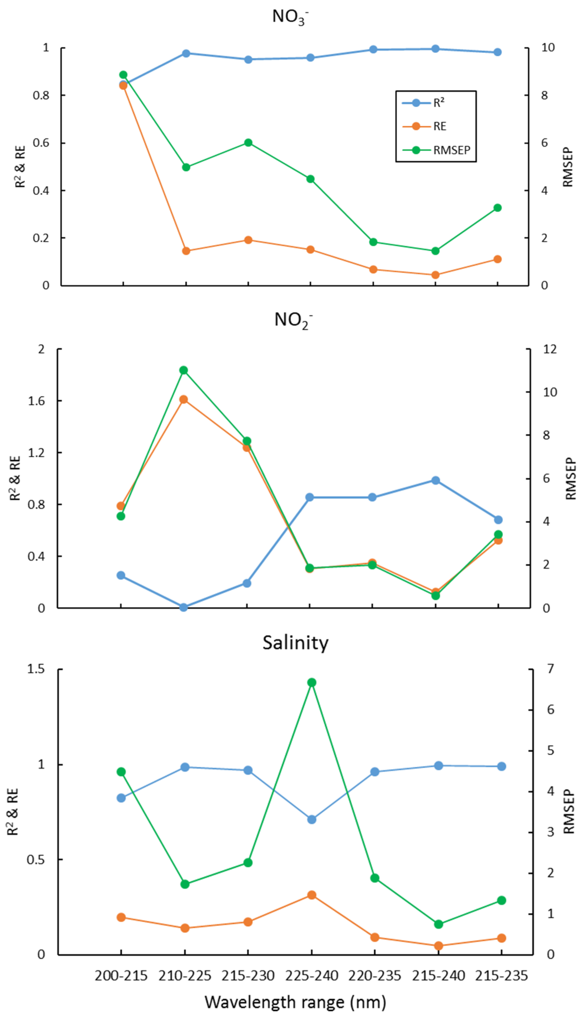
4.2. Wavelength Selection

The wavelength selection is carried out to choose a subset of spectral channels with which the established calibration model can give the minimum errors of the prediction. The optimal wavelength selection offers two clear benefits. Firstly, it has been shown that the inclusion of uninformative wavelengths in the training process negatively affects the accuracy of predictions and model interpretability [48,49]. Secondly, from a more practical point of view, the identification of a few wavelengths, or regions of the optical spectrum, that contain information about chemical species, significantly reduces the time and cost associated with their measurement and enables the development of portable and high-speed optical sensors.

We used interval partial least squares (iPLS) to optimize the wavelength selection proposed by Norgaard et al. (2000) [50], which is to split the spectrum into different intervals and treat each interval as a variable, then the RMSEP, R², and RE for each interval was calculated. The interval with maximal R², and minimum RMSEP and RE, was chosen as the optimal wavelength interval. Here, the 200–300nm wavelength is equally divided into equal subintervals of 16 nm, 200–215 nm, 210–225, 220–235, …, 285–300 nm. Then the wavelength range with the lowest RMSEP value was chosen for further optimization using one-sided symmetrical optimization. The results of the PLS2 for several wavelength ranges are shown in Figure 2. This suggests that the optimal wavelength interval is 215–240 nm, which gives the maximal R², and minimal RE and RMSEP, for NO₃⁻, NO₂⁻, and salinity simultaneously. The plots of these predicted concentrations versus actual concentrations using the PLS2 model are shown in Figure 3. As can be seen, the predicted NO₃⁻, NO₂⁻, and salinity predicted are linearly correlated with the actual values, and all the correlation coefficients are > 0.98 (Figure 3). As both the PLS1 and PLS2 models have 4 factors, the results of the PLS1 are the same as the PLS2. For reducing the complexity and computation time of the model, we recommend using the PLS2 model and wavelength of 215–240 nm for calibration and prediction.

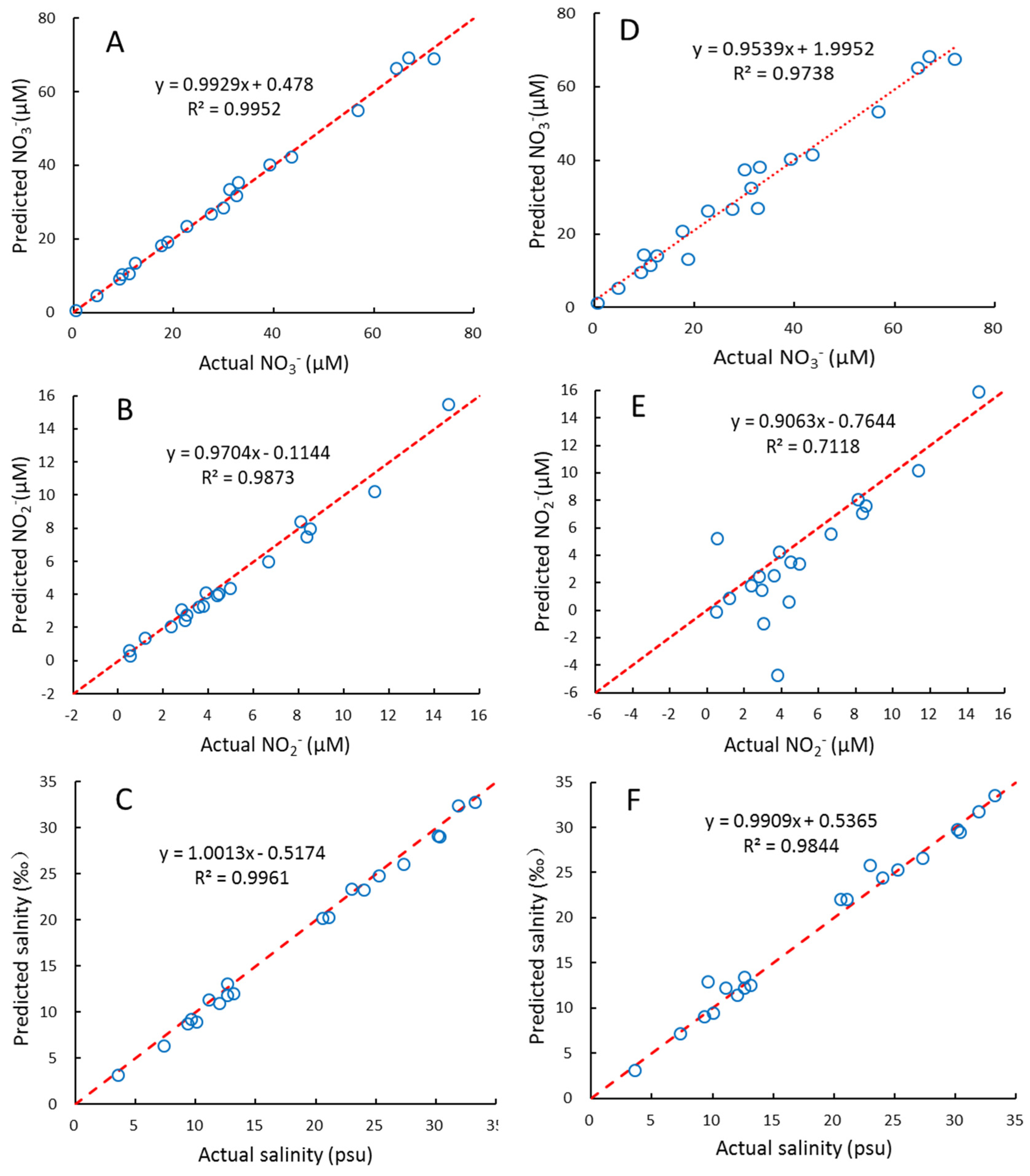
4.3. Comparison of PLS2 and CLS Regressions

For comparison, we also built a CLS model to fit the NO₃⁻, NO₂⁻, and salinity based on Equation (4). The results obtained for the samples of the prediction set are shown in Figure 3. For NO₃⁻ and salinity, the results of CLS are also satisfactory. It is similar to previous studies [9,40,42], in which different CLS algorithms were used to fit NO₃⁻ concentrations and salinity in seawater. However, for several samples with low NO₂⁻ concentrations, the CLS model is less predictive than the PLS2 model. The reason for this may be that NO₂⁻ concentrations in seawater are significantly lower than NO₃⁻, and thus, NO₂⁻ is more susceptible to the interference of sea salt, CDOM, hydrogen sulfide, and other unknown substances. Instead, PLS regression, as an indirect chemometric method, can lead to robust results even if not all the constituents are known [22,23].

4.4. Evaluation of the PLS2 Model

From the experimental data illustrated in Table 1, NO₃⁻, NO₂⁻, and salinity within the range of 0–85.62 μM, 0–20.12 μM, and 0–33.90 psu can be determined accurately by the PLS model. When NO₃⁻ concentration is higher than 100 μM, we suggest using a cuvette with a 1.0 or 2.0 cm pathlength instead of 3.0 cm in case the absorbance tends to saturate. To further evaluate the accuracy of the PLS2 model, recovery studies were carried out on seawater samples, to which known amounts of NO₃⁻ and NO₂⁻ were added (

Table 3. Recoveries of NO₃⁻ and NO₂⁻ in spiked seawater samples.

Spiked (μM)		Found (μM)		Recovery (%)
NO3−	NO2−	NO3−	NO2−	NO3−	NO2−
3.53	2.10	3.22	1.92	109.74	109.36
10.95	14.20	11.23	13.83	97.50	102.66
19.46	1.94	18.83	2.43	103.36	79.97
28.15	6.28	29.26	6.35	96.22	98.85
28.78	3.83	28.18	4.27	102.11	89.75
37.82	5.66	37.17	5.98	101.76	94.69
46.62	7.44	45.90	7.45	101.57	99.93
55.17	9.18	54.54	9.26	101.16	99.13

). The percentage recovery for spiked samples ranged between 80 and 110%. The comparatively higher deviations from spiked concentrations were obtained from samples with low NO₃⁻ or NO₂⁻ concentrations. The detection limits of NO₃⁻ and NO₂⁻ in seawater were calculated as three times the standard deviation of 10 replicate analyses of a low-nutrient (surface) seawater. The standard deviation of the measurements was 0.07 and 0.10 μM for NO₃⁻ and NO₂⁻, which gives NO₃⁻ and NO₂⁻ detection limits of 0.21 and 0.30 μM, respectively. The relative standard deviations for 10 repetitive analyses (n = 10) of a standard solution (3.71 μM NO₃⁻ + 1.48 μM NO₂⁻) were 3.16% and 7.42%, and another solution of 20.75 μM NO₃⁻ and 6.28 μM NO₂⁻ gave the relative standard deviation of 0.61% and 2.39%. Hence, the proposed method is quite precise for the quantitative determination of NO₃⁻ and NO₂⁻ in seawater, although the detection limits are comparatively higher than that of most colorimetric methods based on the Griess reaction [4,5,6]. Most importantly, it offers a simple, fast, and reagent-free method for the simultaneous determination of NO₃⁻ and NO₂⁻.

4.5. Application and Comparison of the Predicted Results with Conventional Wet-Chemical Analyses

To evaluate the analytical applicability of the proposed PLS2 model, it was applied to the simultaneous determination of NO₃⁻, NO₂⁻, and salinity in water samples collected from the Changjiang estuary. These samples were filtered using 0.2μm polycarbonate filters to eliminate the interference from turbidity. For comparison, the NO₃⁻ and NO₂⁻ concentrations were also measured by conventional wet-chemical analyses (colorimetric Griess assay). The results are shown in

Table 4. The predicted values of NO₃⁻, NO₂⁻, and salinity (average ± 1 standard deviation of three replicate analyses) using the PLS2 model in seawater samples of the Changjiang Estuary.

Sample	NO3− (μM)	NO2− (μM)	Salinity (psu)
1	11.96 ± 0.13 (10.55 ± 0.54)	4.63 ± 0.13 (3.59 ± 0.12)	23.53 ± 0.04
2	75.73 ± 0.32 (74.68 ± 1.26)	3.73 ± 0.17 (3.14 ± 0.09)	17.07 ± 0.37
3	51.60 ± 0.26 (52.19 ± 1.77)	2.47 ± 0.19 (1.57 ± 0.21)	21.30 ± 0.43
4	33.36 ± 0.08 (31.85 ± 0.89)	7.41 ± 0.08 (6.53 ± 1.12)	23.83 ± 0.01
5	19.36 ± 0.12 (20.73 ± 0.63)	1.27 ± 0.11 (0.67 ± 0.09)	35.29 ± 0.21
6	21.27 ± 0.11 (20.06 ± 0.42)	0.11 ± 0.16 (0.26 ± 0.04)	29.13 ± 0.21
7	73.67 ± 0.09 (72.12 ± 1.02)	0.47 ± 0.13 (1.03 ± 0.13)	3.66 ± 0.04
8	14.18 ± 0.14 (12.53 ± 0.56)	−0.35 ± 0.11 (0.49 ± 0.08)	31.99 ± 0.21
9	68.88 ± 0.28 (67.18 ± 1.55)	5.92 ± 0.22 (4.25 ± 0.06)	20.56 ± 0.16

Notes: NO₃⁻ and NO₂⁻ concentrations shown in brackets were determined by the Griess assay.

, which suggests the good agreement of both methods.

It should be noted that the in situ UV absorption spectrum, which is obtained at different temperatures, should be corrected according to the temperature dependence of bromide or sea salt, as suggested by Sakamoto et al. (2009, 2017) [41,51]. However, here, we measured the UV absorption spectra in a laboratory at room temperature (~25 °C). Therefore, there is no need to perform the temperature and pressure correction.

5. Conclusions

A direct, reagent-free, ultraviolet spectroscopic was introduced for the simultaneous determination of NO₃⁻, NO₂⁻, and salinity in seawater. A PLS model was built for the resolution of the high overlapping spectra. This method has detection limits of 0.21 and 0.3 μM for NO₃⁻ and NO₂⁻. It can be successfully used to determine NO₃⁻, NO₂⁻, and salinity, especially in estuarine and coastal waters with varying CDOM characteristics and different salinities. The simplicity, precision, and fast response time suggest that the proposed PLS model can be a valuable and cheap alternative to other chemical methods and can be used to build NO₃⁻ and NO₂⁻ sensors for seawater.

References

1. Arrigo, K.R. Marine microorganisms and global nutrient cycles. Nature 2005, 437, 349–355. [Google Scholar] [CrossRef] [PubMed]
2. Falkowski, P.G.; Barber, R.T.; Smetacek, V.V. Biogeochemical Controls and Feedbacks on Ocean Primary Production. Science 1998, 281, 200–207. [Google Scholar] [CrossRef] [PubMed] [Green Version]
3. Vollenweider, R.A.; Marchetti, R.; Viviani, R. The problems of the Emilia Romagna coastal waters: Facts and interpretations. Mar. Coast. Eutrophication 1992, 21–33. [Google Scholar] [CrossRef]
4. Ma, J.; Adornato, L.; Byrne, R.H.; Yuan, D. Determination of nanomolar levels of nutrients in seawater. Trends Anal. Chem. 2014, 60, 1–15. [Google Scholar] [CrossRef]
5. Singh, P.; Singh, M.K.; Beg, Y.R.; Nishad, G.R. A review on spectroscopic methods for determination of nitrite and nitrate in environmental samples. Talanta 2019, 191, 364–381. [Google Scholar] [CrossRef] [PubMed]
6. Wang, Q.H.; Yu, L.J.; Liu, Y.; Lin, L.; Lu, R.G.; Zhu, J.P.; He, L.; Lu, Z.L. Methods for the detection and determination of nitrite and nitrate: A review. Talanta 2017, 165, 709–720. [Google Scholar] [CrossRef]
7. Armstrong, F.A.J. Determination of Nitrate in Water Ultraviolet Spectrophotometry. Anal. Chem. 1963, 35, 1292–1294. [Google Scholar] [CrossRef]
8. American Public Health Association (APHA); American Water Works Association (AWWA); Water Environment Federation (WEF). Standard Methods for the Examination of Water and Wastewater; American Public Health Association: Washington, DC, USA, 1912. [Google Scholar]
9. Johnson, K.S.; Coletti, L.J. In situ ultraviolet spectrophotometry for high resolution and long-term monitoring of nitrate, bromide and bisulfide in the ocean. Deep Sea Res. Part I 2002, 49, 1291–1305. [Google Scholar] [CrossRef]
10. Thomas, O.; Gallot, S.; Mazas, N. Ultraviolet multiwavelength absorptiometry (UVMA) for the examination of natural waters and waste waters: Part II: Determination of nitrate. Fresenius J. Anal. Chem. 1990, 338, 238–240. [Google Scholar] [CrossRef]
11. Huebsch, M.; Grimmeisen, F.; Zemann, M.; Fenton, O.; Richards, K.G.; Jordan, P.; Sawarieh, A.; Blum, P.; Goldscheider, N. Technical Note: Field experiences using UV/VIS sensors for high-resolution monitoring of nitrate in groundwater. Hydrol. Earth Syst. Sci. 2015, 19, 1589–1598. [Google Scholar] [CrossRef] [Green Version]
12. Zielinski, O.; Fiedler, B.; Heuermann, R.; Kortzinger, A.; Munderloh, K. A new nitrate continuous observation sensor for autonomous sub-surface applications: Technical design and first results. In Proceedings of the Oceans 2007, Aberdeen, UK, 18–21 June 2007; pp. 1–4. [Google Scholar]
13. Gruber, N. Chapter 1—The Marine Nitrogen Cycle: Overview and Challenges. In Nitrogen in the Marine Environment, 2nd ed.; Capone, D.G., Bronk, D.A., Mulholland, M.R., Carpenter, E.J., Eds.; Academic Press: San Diego, CA, USA, 2008; pp. 1–50. [Google Scholar]
14. Casciotti, K.L.; Böhlke, J.K.; Mcilvin, M.R.; Mroczkowski, S.J.; Hannon, J.E. Oxygen Isotopes in Nitrite: Analysis, Calibration, and Equilibration. Anal. Chem. 2007, 79, 2427–2436. [Google Scholar] [CrossRef] [PubMed]
15. Casciotti, K.L.; Buchwald, C.; Mcilvin, M. Implications of nitrate and nitrite isotopic measurements for the mechanisms of nitrogen cycling in the Peru oxygen deficient zone. Deep Sea Res. Part I 2013, 80, 78–93. [Google Scholar] [CrossRef]
16. Hu, H.; Bourbonnais, A.; Larkum, J.; Bange, H.W.; Altabet, M.A. Nitrogen cycling in shallow low-oxygen coastal waters off Peru from nitrite and nitrate nitrogen and oxygen isotopes. Biogeosciences 2016, 13, 7257–7299. [Google Scholar] [CrossRef] [Green Version]
17. Lam, P.; Lavik, G.; Jensen, M.M.; Vossenberg, J.V.D.; Schmid, M.; Woebken, D.; Gutiérrez, D.; Amann, R.; Jetten, M.S.M.; Kuypers, M.M.M. Revising the nitrogen cycle in the Peruvian oxygen minimum zone. Proc. Nat. Acad. Sci. USA 2009, 106, 4752–4757. [Google Scholar] [CrossRef] [Green Version]
18. Morrison, J.M.; Codispoti, L.A.; Smith, S.L.; Wishner, K.; Flagg, C.; Gardner, W.D.; Gaurin, S.; Naqvi, S.W.A.; Manghnani, V.; Prosperie, L. The oxygen minimum zone in the Arabian Sea during 1995. Deep Sea Res. Part II 1999, 46, 1931. [Google Scholar] [CrossRef]
19. Langergraber, G.; Fleischmann, N.; Hofstaedter, F. A multivariate calibration procedure for UV/VIS spectrometric quantification of organic matter and nitrate in wastewater. Water Sci. Technol. 2003, 47, 63–71. [Google Scholar] [CrossRef] [Green Version]
20. Rieger, L.; Langergraber, G.; Thomann, M.; Fleischmann, N.; Siegrist, H. Spectral in-situ analysis of NO2, NO3, COD, DOC and TSS in the effluent of a WWTP. Water Sci. Technol. 2004, 50, 143–152. [Google Scholar] [CrossRef] [PubMed]
21. Rieger, L.; Vanrolleghem, P.A.; Langergraber, G.; Kaelin, D.; Siegrist, H. Long-term evaluation of a spectral sensor for nitrite and nitrate. Water Sci. Technol. 2008, 57, 1563. [Google Scholar] [CrossRef]
22. Haaland, D.M.; Thomas, E.V. Partial least-squares methods for spectral analyses. 1. Relation to other quantitative calibration methods and the extraction of qualitative information. Anal. Chem. 1988, 60, 1193–1202. [Google Scholar] [CrossRef]
23. Otto, M. Chemometrics: Statistics and Computer Application in Analytical Chemistry; Wiley-VCH Verlag GmbH: Weinheim, Germany, 1999. [Google Scholar]
24. Beebe, K.R.; Kowalski, B.R. An Introduction to Multivariate Calibration and Analysis. Anal. Chem. 1987, 59, 1007A–1017A. [Google Scholar] [CrossRef]
25. Martens, H.; Naes, T. Multivariate Calibration; Wiley & Sons: Chichester, UK, 1989. [Google Scholar]
26. Wold, S.; Sjöström, M.; Eriksson, L. PLS-regression: A basic tool of chemometrics. Chemom. Intell. Lab. Syst. 2001, 58, 109–130. [Google Scholar] [CrossRef]
27. Manne, R. Analysis of Two PLS Algorithms for Multivariate Calibration. Chemom. Intell. Lab. Syst. 1987, 2, 187–197. [Google Scholar] [CrossRef]
28. Khajehsharifi, H.; Mousavi, M.F.; Ghasemi, J.; Shamsipur, M. Kinetic spectrophotometric method for simultaneous determination of selenium and tellurium using partial least squares calibration. Anal. Chim. Acta 2004, 512, 369–373. [Google Scholar] [CrossRef]
29. Tewari, J.; Strong, R.; Boulas, P. At-line determination of pharmaceuticals small molecule’s blending end point using chemometric modeling combined with Fourier transform near infrared spectroscopy. Spectrochim. Acta Part A 2017, 173, 886–891. [Google Scholar] [CrossRef]
30. Abdel-Rahman, E.M.; Mutanga, O.; Odindi, J.; Adam, E.; Odindo, A.; Ismail, R. Estimating Swiss chard foliar macro- and micronutrient concentrations under different irrigation water sources using ground-based hyperspectral data and four partial least squares (PLS)-based (PLS1, PLS2, SPLS1 and SPLS2) regression algorithms. Comput. Electron. Agric. 2017, 132, 21–33. [Google Scholar] [CrossRef]
31. Andries, J.P.M.; Heyden, Y.V.; Buydens, L.M.C. Predictive-property-ranked variable reduction with final complexity adapted models in partial least squares modeling for multiple responses. Anal. Chem. 2013, 85, 5444–5453. [Google Scholar] [CrossRef]
32. Thurman, E.M. Organic Geochemistry of Natural Waters; M.Nijhoff/Dr. W. Junk Publishers: Dordrecht, The Netherlands, 1985. [Google Scholar]
33. Kirk, J.T. Light and Photosynthesis in Aquatic Ecosystems; Cambridge University Press: Cambridge, UK, 1994. [Google Scholar]
34. Hansell, D.A.; Carlson, C.A. Biogeochemistry of Marine Dissolved Organic Matter; Academic Press: London, UK, 2014. [Google Scholar]
35. Nelson, N.B.; Siegel, D.A. The global distribution and dynamics of chromophoric dissolved organic matter. Annu. Rev. Mar. Sci. 2013, 5, 447–476. [Google Scholar] [CrossRef] [PubMed] [Green Version]
36. Twardowski, M.S.; Boss, E.; Sullivan, J.M.; Donaghay, P.L. Modeling the spectral shape of absorption by chromophoric dissolved organic matter. Mar. Chem. 2004, 89, 69–88. [Google Scholar] [CrossRef]
37. Guenther, E.A.; Johnson, K.S.; Coale, K.H. Direct ultraviolet spectrophotometric determination of total sulfide and iodide in natural waters. Anal. Chem. 2001, 73, 3481–3487. [Google Scholar] [CrossRef] [PubMed]
38. Helms, J.R.; Stubbins, A.; Ritchie, J.D.; Minor, E.C.; Kieber, D.J.; Mopper, K. Absorption spectral slopes and slope ratios as indicators of molecular weight, source, and photobleaching of chromophoric dissolved organic matter. Limnol. Oceanogr. 2008, 53, 955–969. [Google Scholar] [CrossRef] [Green Version]
39. Li, P.; Hur, J. Utilization of UV-Vis spectroscopy and related data analyses for dissolved organic matter (DOM) studies: A review. Crit. Rev. Environ. Sci. Technol. 2017, 47, 131–154. [Google Scholar] [CrossRef]
40. Frank, C.; Meier, D.; Voß, D.; Zielinski, O. Computation of nitrate concentrations in coastal waters using an in situ ultraviolet spectrophotometer: Behavior of different computation methods in a case study a steep salinity gradient in the southern North Sea. Methods Oceanogr. 2014, 9, 34–43. [Google Scholar] [CrossRef]
41. Sakamoto, C.M.; Johnson, K.S.; Coletti, L.J. Improved algorithm for the computation of nitrate concentrations in seawater using an in situ ultraviolet spectrophotometer. Limnol. Oceanogr. Methods 2009, 7, 32–143. [Google Scholar] [CrossRef]
42. Zielinski, O.; Voß, D.; Saworski, B.; Fiedler, B.; Körtzinger, A. Computation of nitrate concentrations in turbid coastal waters using an in situ ultraviolet spectrophotometer. Sea Res. 2011, 65, 456–460. [Google Scholar] [CrossRef]
43. Press, W.; Flannery, B.; Teukolsky, S.; Vetterling, W. Numerical Recipes: The Art of Scientific Computing; Cambridge University Press: Cambridge, UK, 1986. [Google Scholar]
44. Sen, A. Srivastava, M. Unequal Variances, Regression Analysis; Springer: Berlin, Germany, 1990; pp. 111–131. [Google Scholar]
45. Stone, M.P. Cross-validatory choice and assessment of statistical predictions. Inst. Phys. Pub. 1974, 36, 111–133. [Google Scholar] [CrossRef]
46. Tenenhaus, M. La Régression PLS: Théorie et Pratique; Editions Technip: Paris, France, 1998. [Google Scholar]
47. Abdi, H. Partial least squares regression and projection on latent structure regression (PLS-regression). Comput. Stat. 2010, 2, 97–106. [Google Scholar] [CrossRef]
48. Chang, H.; Zhu, L.; Lou, X.; Meng, X.; Guo, Y.; Wang, Z. Local Strategy Combined with a Wavelength Selection Method for Multivariate Calibration. Sensors 2016, 16, 827. [Google Scholar] [CrossRef] [PubMed] [Green Version]
49. Mamouei, M.; Budidha, K.; Baishya, N.; Qassem, M.; Kyriacou, P. Comparison of wavelength selection methods for in-vitro estimation of lactate: A new unconstrained, genetic algorithm-based wavelength selection. Sci. Rep. 2020, 10, 16905. [Google Scholar] [CrossRef] [PubMed]
50. Nielsen, J.P.; Munck, L.; Engelsen, S.B.; Norgaard, L.; Saudland, A.; Wagner, J. Interval Partial Least-Squares Regression (iPLS): A Comparative Chemometric Study with an Example from Near-Infrared Spectroscopy. Appl. Spectrosc. 2000, 54, 413–419. [Google Scholar]
51. Sakamoto, C.M.; Johnson, K.S.; Coletti, L.J.; Jannasch, H.W. Pressure correction for the computation of nitrate concentrations in seawater using an in situ ultraviolet spectrophotometer. Limnol. Ocanogr. Methods 2017, 15, 897–902. [Google Scholar] [CrossRef] [Green Version]
Figure 1. Absorption spectra of NO3, NO2, and sea salt (salinity).
Molecules 26 03685 g001
Figure 2. R2, RE, and RMSEP of NO3, NO2, and salinity for different wavelength ranges.
Molecules 26 03685 g002
Figure 3. The relationships between the actual and predicted NO3, NO2 and salinity of samples in prediction set using PLS2 model (AC) and CLS model (DF). Red dash lines indicate ratio of actual: predicted value = 1:1.
Molecules 26 03685 g003