Figure 1.
A plot of the surface tension () of the aqueous solutions of CTAB + TX100 + FC1 mixture at the constant concentration of the binary mixture CTAB + TX100 () and = 60 mN/m (m1 (60)) vs. the logarithm of FC1 concentration (). Points 1 correspond to the measured values, curves 2, 3 and 4 correspond to the values calculated from the Fainerman and Miller (Equation (3)), the Szyszkowski equation (Equation (1)) and the second order exponential function (Equation (2)), respectively.
Figure 2.
A plot of the surface tension () of the aqueous solutions of CTAB + TX100 + FC1 mixture at the constant concentration of the binary mixture CTAB + TX100 () and = 50 mN/m (m1 (50)) vs. the logarithm of FC1 concentration (). Points 1 correspond to the measured values, curves 2, 3 and 4 correspond the values calculated from the Fainerman and Miller (Equation (3)), the Szyszkowski equation (Equation (1)) and the second order exponential function (Equation (2)), respectively.
Figure 3.
A plot of the surface tension () of the aqueous solutions of CTAB + TX100 + FC2 mixture at the constant concentration of the binary mixture CTAB + TX100 () and = 60 mN/m (m2 (60)) vs. the logarithm of FC2 concentration (). Points 1 correspond to the measured values, curves 2, 3 and 4 correspond the values calculated from the Fainerman and Miller (Equation (3)), the Szyszkowski equation (Equation (1)) and the second order exponential function (Equation (2)), respectively.
Figure 4.
A plot of the surface tension () of the aqueous solutions of CTAB + TX100 + FC2 mixture at the constant concentration of the binary mixture CTAB + TX100 () and = 50 mN/m (m2 (50)) vs. the logarithm of FC2 concentration (). Points 1 correspond to the measured values, curves 2, 3 and 4 correspond the values calculated from the Fainerman and Miller (Equation (3)), the Szyszkowski equation (Equation (1)) and the second order exponential function (Equation (2)), respectively.
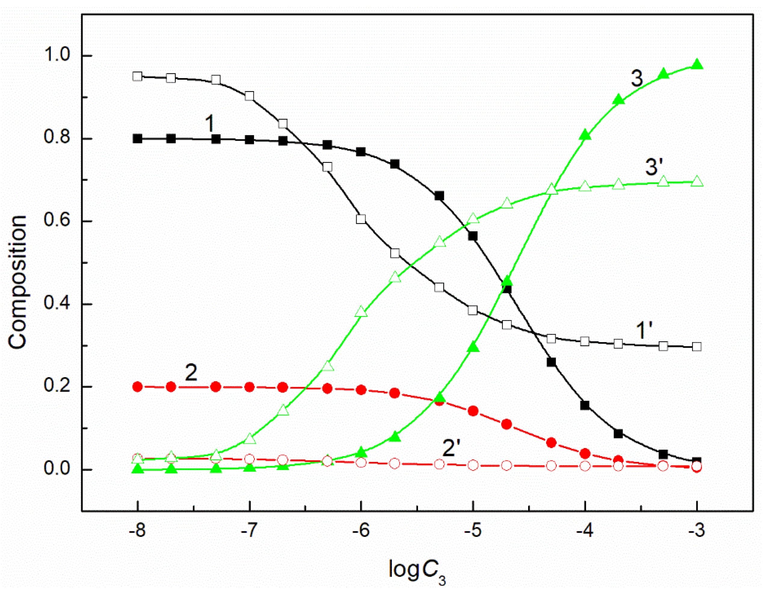
Figure 5.
A plot of the composition of the ternary mixture including CTAB, TX100 and FC1 in the monolayer (curves 1–3) and in the bulk phase (curves 1’–3’) at the constant and = 60 mN/m vs. the logarithm of the FC1 concentration (). Curves 1, 1’ correspond to CTAB, curves 2, 2’ correspond to TX100 and curves 3, 3’ to FC1.
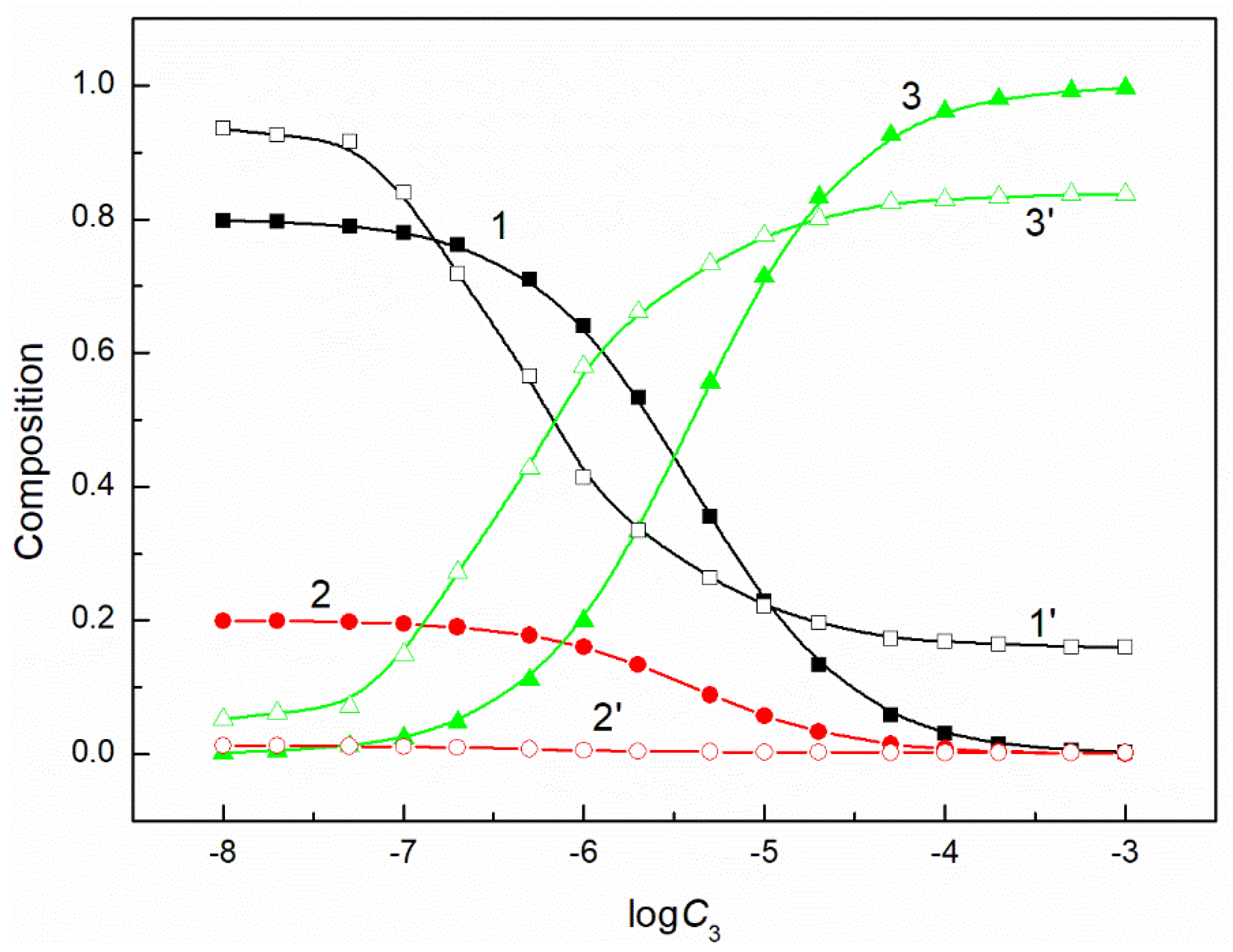
Figure 6.
A plot of the composition of the ternary mixture including CTAB, TX100 and FC1 in the monolayer (curves 1–3) and in the bulk phase (curves 1’–3’) at the constant and = 50 mN/m vs. the logarithm of the FC1 concentration (). Curves 1, 1’ correspond to CTAB, curves 2, 2’ correspond to TX100 and curves 3–3’ to FC1.
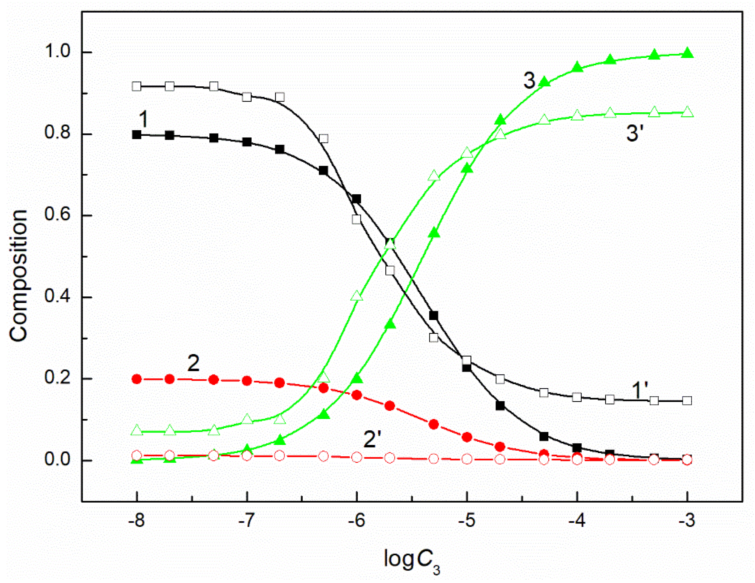
Figure 7.
A plot of the composition of the ternary mixture including CTAB, TX100 and FC2 in the monolayer (curves 1–3) and in the bulk phase (curves 1’–3’) at the constant and = 60 mN/m vs. the logarithm of the FC2 concentration (). Curves 1, 1’ correspond to CTAB, curves 2, 2’ correspond to TX100 and curves 3–3’ to FC2.
Figure 8.
A plot of the composition of the ternary mixture including CTAB, TX100 and FC2 in the monolayer (curves 1–3) and in the bulk phase (curves 1’–3’) at the constant and = 50 mN/m vs. the logarithm of the FC2 concentration (). Curves 1, 1’ correspond to CTAB, curves 2, 2’ correspond to TX100 and curves 3–3’ to FC2.
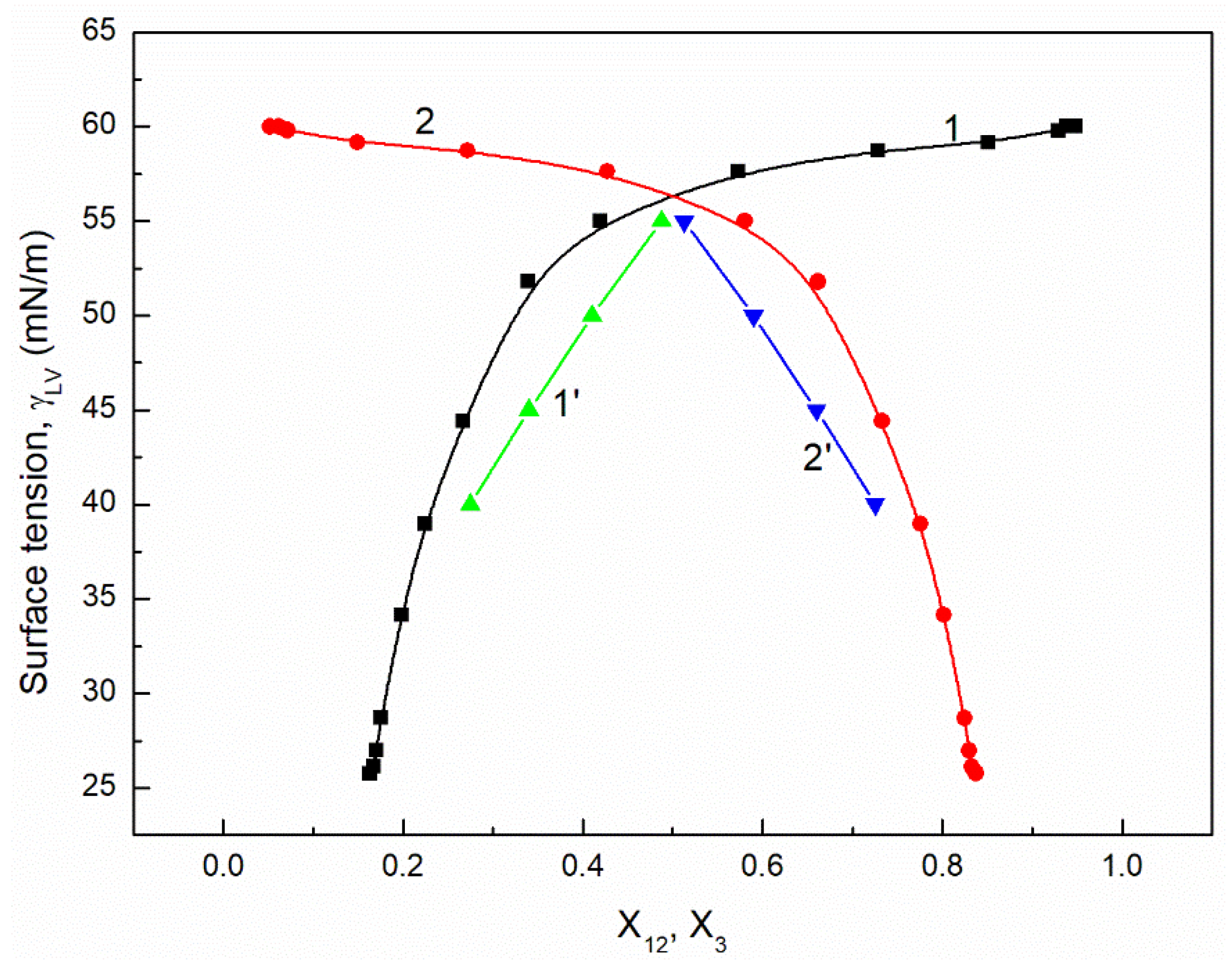
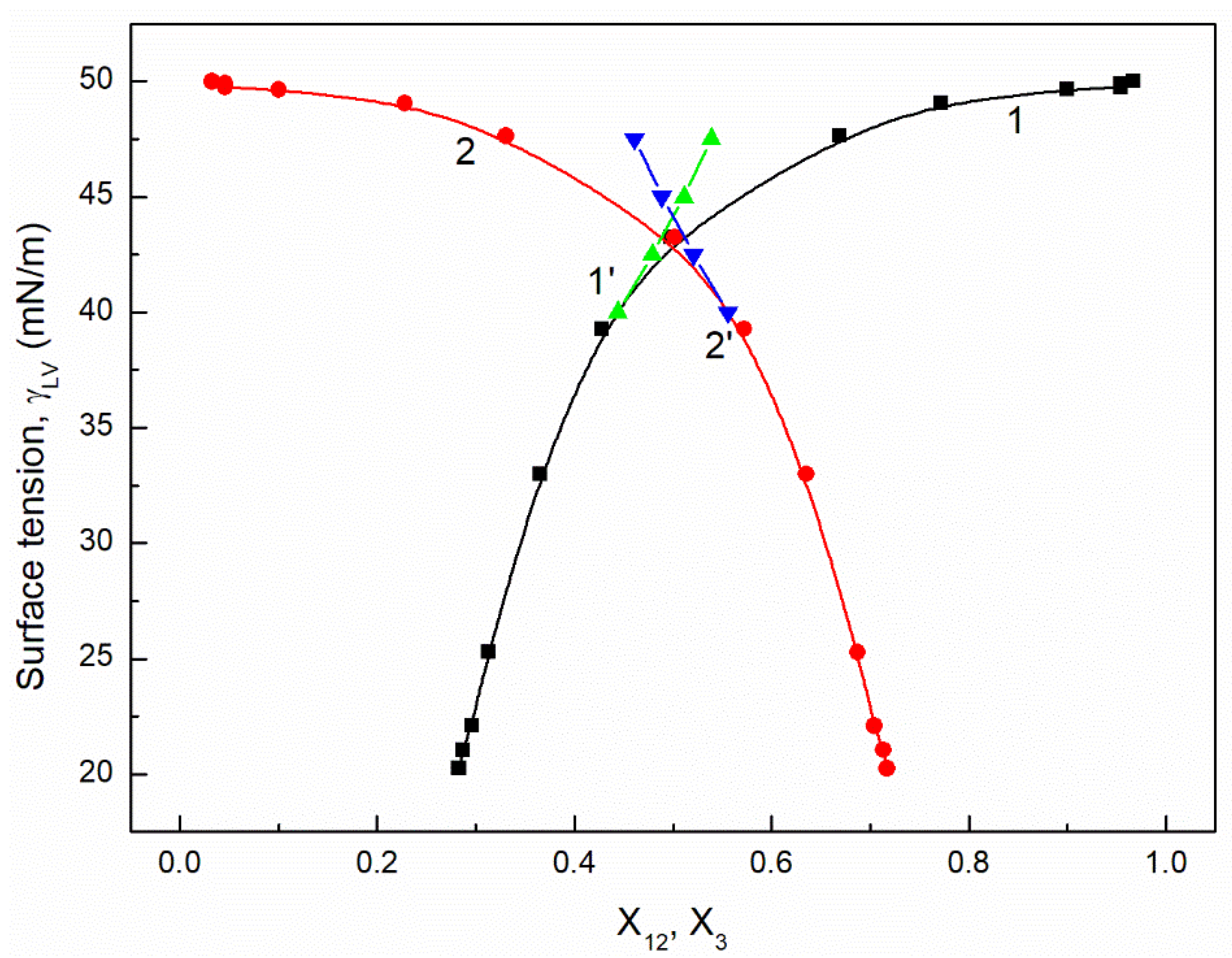
Figure 9.
A plot of the surface tension () of the aqueous solutions of CTAB + TX100 + FC1 mixture at the constant concentration of the binary mixture CTAB + TX100 () and = 60 mN/m (m1 (60) vs. the composition of the ternary mixture in the monolayer ( and ) determined based on the contribution of the particular surfactant in the mixture to the reduction of the water surface tension (curves 1 and 2) and calculated from Equation (5) (curves 1’ and 2’). corresponds to the sum of the CTAB () and TX100 () fractions and corresponds to the FC1 fraction.
Figure 10.
A plot of the surface tension () of the aqueous solutions of CTAB + TX100 + FC1 mixture at the constant concentration of the binary mixture CTAB + TX100 () and = 50 mN/m (m1 (50)) vs. the composition of the ternary mixture in the monolayer ( and ) determined based on the contribution of the particular surfactant in the mixture to the reduction of the water surface tension (curves 1 and 2) and calculated from Equation (5) (curves 1’ and 2’). corresponds to the sum of the CTAB () and TX100 () fractions and corresponds to the FC1 fraction.
Figure 11.
A plot of the surface tension () of the aqueous solutions of CTAB + TX100 + FC2 mixture at the constant concentration of the binary mixture CTAB + TX100 () and = 60 mN/m (m2 (60)) vs. the composition of the ternary mixture in the monolayer ( and ) determined based on the contribution of the particular surfactant in the mixture to the reduction of the water surface tension (curves 1 and 2) and calculated from Equation (5) (curves 1’ and 2’). corresponds to the sum of the CTAB () and TX100 () fractions and corresponds to the FC2 fraction.
Figure 12.
A plot of the surface tension () of the aqueous solutions of CTAB + TX100 + FC2 mixture at the constant concentration of the binary mixture CTAB + TX100 () and = 50 mN/m (m2 (50)) vs. the composition of the ternary mixture in the monolayer ( and ) determined based on the contribution of the particular surfactant in the mixture to the reduction of the water surface tension (curves 1 and 2) and calculated from Equation (5) (curves 1’ and 2’). corresponds to the sum of the CTAB () and TX100 () fractions and corresponds to the FC2 fraction.
Figure 13.
A plot of the Gibbs surface excess concentration of FC1 () calculated from Equation (9) based on the measured surface tension of the ternary mixture at the constant concentration of the CTAB + TX100 at equal 60 mN/m (curve 1) and 50 mN/m (curve 2) and on the contribution of FC1 to the reduction of water surface tension (curve 1’corresponds to = 60 mN/m and curve 2’corresponds to = 50 mN/m) vs. the logarithm of the FC1 concentration ().
Figure 14.
A plot of the Gibbs surface excess concentration of FC1 () calculated from Equation (9) based on the measured surface tension of the ternary mixture at the constant concentration of the CTAB + TX100 at equal 60 mN/m (curve 1) and 50 mN/m (curve 2) and on the contribution of FC2 to the reduction of water surface tension (curve 1’corresponds to = 60 mN/m and curve 2’ corresponds to = 50 mN/m) vs. the logarithm of the FC2 concentration ().
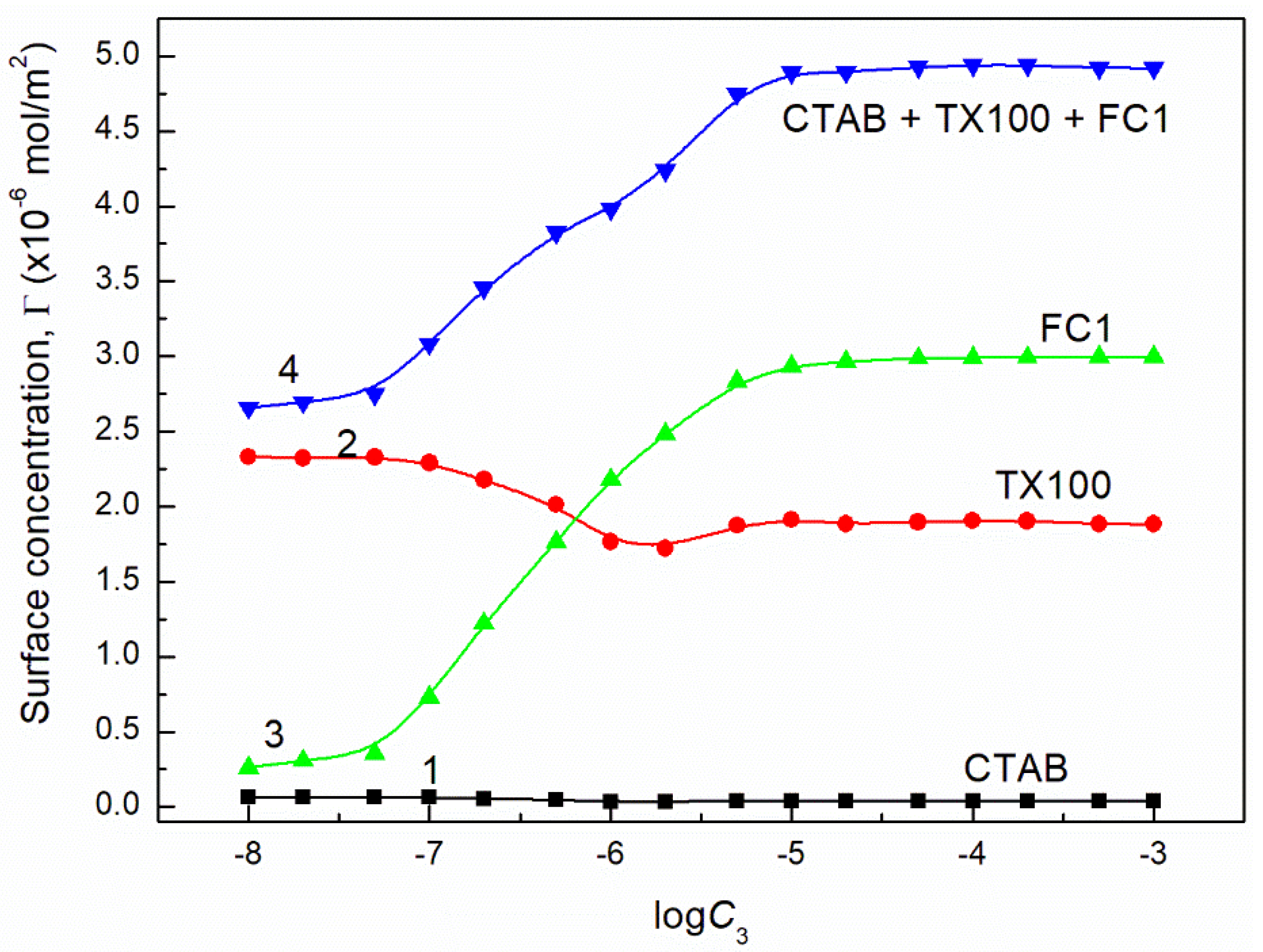
Figure 15.
A plot of the concentration of CTAB (curve 1), TX100 (curve 2), FC1 (curve 3) and their sum (curve 4) in the mixed monolayer at the water-air interface formed by the CTAB + TX100 + FC1 mixture at the constant concentration of the binary CTAB + TX100 mixture () and = 60 mN/m as well as calculated from Equation (12) based the contribution of the given surfactant to the reduction of water surface tension vs. the logarithm of the FC1 concentration ().
Figure 16.
A plot of the concentration of CTAB (curve 1), TX100 (curve 2), FC1 (curve 3) and their sum (curve 4) in the mixed monolayer at the water-air interface formed by the CTAB + TX100 + FC1 mixture at the constant concentration of the binary CTAB + TX100 mixture () and = 50 mN/m as well as calculated from Equation (12) based on the contribution of the given surfactant to the reduction of water surface tension vs. the logarithm of the FC1 concentration ().
Figure 17.
A plot of the concentration of CTAB (curve 1), TX100 (curve 2), FC2 (curve 3) and their sum (curve 4) in the mixed monolayer at the water-air interface formed by the CTAB + TX100 + FC1 mixture at the constant concentration of the binary CTAB + TX100 mixture () and = 60 mN/m as well as calculated from Equation (12) based on the contribution of the given surfactant to the reduction of water surface tension vs. the logarithm of the FC2 concentration ().
Figure 18.
A plot of the concentration of CTAB (curve 1), TX100 (curve 2), FC2 (curve 3) and their sum (curve 4) in the mixed monolayer at the water−air interface formed by the CTAB + TX100 + FC1 mixture at the constant concentration of the binary CTAB + TX100 mixture () and = 50 mN/m as well as calculated from Equation (12) based on the contribution of the given surfactant to the reduction of water surface tension vs. the logarithm of the FC2 concentration ().
Table 1.
The values of the constants of the second order exponential function describing the relationship between the surface tension and the fluorocarbon surfactant concentration (Equation (2)) of CTAB + TX100 + FC1 (m1 (60), m1 (50)) and CTAB + TX100 + FC2 (m2 (60), m2 (50)) mixtures at CTAB + TX100 equal to 60 and 50 mN/m, respectively.
| Mixture | | | | | |
|---|
|
m1 (60)
| 17.39734 | 16.53115 | 3.75681 × 10⁻⁶ | 2.84267 × 10⁻⁵ | 26.00475 |
|
m1 (50)
| 18.94709 | 4.93928 | 1.10939 × 10⁻⁵ | 1.10626 × 10⁻⁴ | 26.14665 |
|
m2 (60)
| 15.37929 | 24.31508 | 5.25560 × 10⁻⁶ | 3.47902 × 10⁻⁵ | 20.52881 |
|
m2 (50)
| 7.45181 | 22.35440 | 7.41333 × 10⁻⁵ | 1.68900 × 10⁻⁵ | 20.30326 |
Table 2.
The values of the parameters of intermolecular interaction, , (Equation (6)) activity coefficients of CTAB + TX100 mixture, , and fluorocarbon surfactant, (Equations (8) and (9)) and Gibbs excess free energy of mixing, (Equation (7)) of CTAB + TX100 + FC1 (m1 (60), m1 (50)) and CTAB + TX100 + FC2 (m2 (60), m2 (50)) mixtures at CTAB + TX100 equal to 60 and 50 mN/m, respectively, at the different fluorocarbon surfactants’ surface tension.
| Mixture | | | | | |
|---|
|
m1 (60)
| 55 | −7.01610 | 0.15843 | 0.18866 | −4.27016 |
| 50 | −5.21987 | 0.16282 | 0.41528 | −3.07662 |
| 45 | −4.94660 | 0.11637 | 0.56414 | −2.70309 |
| 40 | −4.66777 | 0.08598 | 0.70261 | −2.26693 |
|
m1 (50)
| 47.5 | −12.45280 | 0.06581 | 0.02925 | −7.55158 |
| 45 | −9.73223 | 0.09052 | 0.08508 | −5.92669 |
| 42.5 | −7.68936 | 0.11361 | 0.18539 | −4.66383 |
| 40 | −6.53262 | 0.12019 | 0.29799 | −3.90151 |
|
m2 (60)
| 55 | −6.31109 | 0.209705 | 0.20320 | −3.84336 |
| 50 | −4.85452 | 0.19322 | 0.42806 | −2.87703 |
| 45 | −4.45539 | 0.13754 | 0.61067 | −2.40961 |
| 40 | −4.27784 | 0.09733 | 0.74547 | −2.01515 |
|
m2 (50)
| 47.5 | −11.34600 | 0.08949 | 0.03712 | −6.86813 |
| 45 | −9.29972 | 0.10832 | 0.08809 | −5.66073 |
| 42.5 | −7.79572 | 0.12054 | 0.16714 | −4.73926 |
| 40 | −6.79500 | 0.12230 | 0.26211 | −4.08609 |
Table 3.
The values of the standard Gibbs free energy of adsorption (kJ/mol) of FC1 and FC2 (Equations (15) and (16)) and this energy for the mixtures (Equations (17) and (18)).
Table 3.
The values of the standard Gibbs free energy of adsorption (kJ/mol) of FC1 and FC2 (Equations (15) and (16)) and this energy for the mixtures (Equations (17) and (18)).
| Equation | m1 (60) | m1 (50) | m2 (60) | m2 (50) |
|---|
|
Equation (15)
| −42.08 | −38.27 | −41.24 | −38.75 |
|
Equation (16)
| −44.57 | −41.65 | −42.77 | −40.36 |
|
Equation (16)
| −46.57 | −45.79 | −44.78 | −43.64 |
|
Equation (16)
| −44.64 | −38.42 | −42.44 | −43.64 |
|
Equation (17)
| −48.04 | −48.72 | −45.62 | −46.67 |
|
Equation (18)
| −47.92 | −48.30 | −45.93 | −47.55 |


